Boolean Function Complexity and Neural Networks

Proceedings of the 7th WSEAS International Conference on Neural Networks, Cavtat, Croatia, June 12-14, 2006 (pp85-90)

Boolean Function Complexity and Neural Networks ALI ASSI Department of Electrical Engineering, United Arab Emirates University, UAE

P.W.C. PRASAD College of Information Technology, United Arab Emirates University, UAE

AZAM BEG College of Information Technology, United Arab Emirates University, UAE

Abstract - A new neural network (NN) approach is proposed in this paper to estimate the Boolean function (BF) complexity. Large number of randomly generated single output BFs has been used and experimental results show good correlation between the theoretical results and those predicted by the NN model. The proposed model is capable of predicting the number of product terms (NPT) in the BF that gives an indication on its complexity.

. Key-Words: Boolean functions, Neural Networks, Complexity evaluation, Modeling, Simulation

1 Introduction The driving force behind the rapid growth of VLSI technologies has been the constant reduction of the feature size of devices (i.e. the minimum transistor size). According to Moore’s law [1] the number of transistors on a single chip doubles every year, and it has withstood the test of time since Gordon Moore made this observation in 1965. The increasing complexity of modern Very Large Scale Integration (VLSI) circuitry is only manageable through advanced Computer-Aided Design (CAD) systems that allow efficient handling of BFs [2]. The complexity of BFs is one of the central and classical topics in the theory of computation. BFs and their complexity have been investigated for a long time [2], [3], [4]. Mathematicians and computer scientists have long tried to classify BFs according to various complexity measures, such as the minimal size of Boolean circuits needed to compute specific functions [5]. BF representations have direct impact on the computation time and memory requirements in the design of digital circuits. The efficiency of any method depends on the complexity of the BF [6]. Research on the complexity of BFs in non-uniform computation models is now part of one of the most interesting and important areas in the area of theoretical computer science [7]. Based on its BFs representation, it will be useful to have an estimation

of the circuit complexity prior to making decisions on the feasibility of the design [8]. Over the past two decades most of the complexityrelated problems have been solved using various mathematical methods [9]. Apart from this lot of research work has been done on the computational properties of NNs [10], [11] and even on a measure for the complexity of BFs related to their implementation in NNs. The measure of efficiency of the circuit have been addressed within the area of circuit complexity [10],[12], where the complexity of BFs is analyzed in terms of their implementation on different kind of circuits. In solving these problems the important contribution of the NNs is their capacity for learning from experience. The main objective of this paper is to introduce a novel method based on NN for the estimation of the BF complexity for any number of variables and for any NPT. The model will enable the design feasibility and performance to be analyzed without building the circuit. The proposed method is also capable of predicting the maximum complexity and the NPT in the BF that leads to the maximum complexity. In the second section of this paper, background information pertaining to the NNs is given. The proposed complexity model is explained in the third and fourth sections.


2 Overview of Neural Networks NNs mimic the ability of a human brain to find patterns and uncover hidden relationships in data. NNs can be more effective than statistical techniques for organizing data and predicting results, and are very efficient in modeling non-linear systems [13], [14], [15]. An NN is defined as a computational system comprising of simple but highly interconnected processing elements PEs (or neurons) (Fig. 1) [16]. PEs are NN equivalents of biological neurons. Similarly, NN interconnections are equivalents of synapses that connect a neuron to others. Information is processed by the PEs by dynamically responding to their inputs. Unlike conventional computers that process instruction and data stored in the memory in a sequential manner, the NNs produce outputs based on a weighted sum of all inputs in a parallel fashion [13].

Fig. 1. Processing element (PE) – building block of a neural network In Fig. 1 the inputs (i(0)..i(n-1)) to a PE are scaled with weights (w(0) .. w(n-1)) and summed up before being passed through an activation function. The activation function determines whether a PE activates (fires) or not. A sigmoid (non-linear) activation function has an s-shaped output between the limits [0, 1]. The function (1) is defined as [17]: 1 y= (1 + e -x ) (1) Each input of an NN corresponds to a single attribute of the system being modeled. The output of the NN is the prediction we are trying to make. Fig. 2 shows the topology of a simple 5-layer feedforward NN with 2 inputs and one output. The NN has 2 input neurons (PE(ip1), PE(ip2)), three hidden layers with 5 neurons each (PE(hnm) is the mth neuron in nth hidden layer), and one neuron in the output layer (PE(op1)) [13]. The NNM is fullyconnected, meaning; all neurons in one layer connect to all neurons in the next layer.

Fig. 2. Topology of 5-layer feed-forward neural network NNs use different types of learning (or training) mechanisms, the most common of them being supervised learning. In this method of learning, a set of inputs is provided to the NN and its output is compared with the desired output. The difference between the actual and the desired outputs is used to adjust the weights (Fig. 1) to different PEs in the network. The process of adjusting weights is repeated until the output falls within an acceptable range. To ensure a robust NN design, the set of input data and corresponding output data has to be chosen carefully. The input-output data set for an NN is called a training set. Additionally, special attention has to be paid to the formatting and scaling of the data for effective NN training [13]. The available data is divided into training and validation sets. An NN is only trained with the training set. Validation set is run on the NN to verify that the inputs are producing desirable outputs. If the validation phase produces large deviations, the training set or the network structure needs to be re-examined; retraining is required in this case [13].

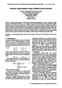
3 Experimental Analysis of Boolean Function Complexity For each variable count n between 1 and 14 inclusive and for each term count between 1 and 2n-1, 100 Sum of Product (SOP) terms were randomly generated and the Colorado University Decision Diagram (CUDD) package [18] was used to determine the complexity of the BF in terms of nodes of its Binary Decision Diagram (BDD) representation. This process was repeated until the BF complexities (i.e. number of nodes) became 1. Then the experimental graphs for BF complexity (Example: for 10 variables, as shown in Figure 3)


were plotted against the product term count for each number of variables.

160 140

Experimental

C om plexity

120

Fig. 4. Inputs and output of the NNM

100 80

4.3 Data Pre-Processing

60 40 20 0 1

51 101 151 201 251 301 351 401 451 501 551 601

Number of Product terms

Fig. 3: Experimental results for Boolean complexity for 10 variables The above graphs indicate that the BF complexity in general increases as the NPT increases. This is clear from the rising edge of the curve. At the end of the rising edge in the graph reaches a maximum complexity. This peak indicates the maximum BF complexity (134) that any BF with 10 variables can have independently of the NPT. Apart from that the peak also specifies the NPT (critical limit) of a BF that leads to the maximum complexity for any BF with 10 variables. The NPT that leads to the maximum for 10 variables is 54. If the NPT increases above the critical limit, as expected, the product terms starts to simplify and the BF complexity will reduce. The Complexity graph shown in Figure 1 indicates that as the NPT increases the complexity of the BF decreases at a slower rate and ultimately reaches 0.

4 Application of Neural Networks to Boolean function Complexity Modeling This section covers the definition and implementation of the Neural Network Model (NNM) for modeling the BF complexity.

4.1 Data collection For the NNM in this paper, the training and validation data sets were obtained by the experiment done in section 3.

4.2 Model Definition The purpose of the NNM in this research was to model the complexity of BFs. Inputs to the NNMs were (1) the number of variables, and (2) NPT (minterms) (Fig. 4).

Pre-processing the training and validations sets takes a considerable amount of resources for a practical and reliably functioning NNM [15], [19]. In our research, the first data pre-processing step was to transform the data set in such a way that inputs have equitable distribution of importance. In other words, the larger absolute values of an input should not have more influence than the inputs with smaller magnitudes [20]. The need of such equitable distribution can be explained with the set of figures shown below. Figure 5 shows the raw (original) data for 2 to 14 variables. Notice that the plots for 2- to 9-variables are hardly visible when all variables are plotted on the same scale. If the data were presented to the NN for training in this case, only 10- to 14- variable cases could be learnt by the NN and 2- to 9-variables values could be ignored. So in order to provide similar importance to all variable values (2 to 14), we performed a logarithmic transformation of the product terms (min-terms) and complexity (number of nodes) inputs. The resulting data is plotted in Figure 6. As we can see now all different plots (from 2 to 14 variables) are in similar ranges and make it easier for NN to learn them. In order to ‘use’ or ‘run’ a trained NN, denormalization and de-transformation has to be done to restore the predicted outputs to the original ranges. Steps employed in 'training' and 'running' the network are summarized here: Steps for Training the NNM: a) Take logarithm of actual values of the inputs and output b) Train the NN with values from step (a) Steps for Using/Running the NNM: a) Take logarithm of the actual values of the input b) Present the values from step (a) to the NNM c) Apply anti-logarithm to the output of the NNM to get the actual result

600

5 Var 6 Var 7 Var

400

8 Var 9 Var

200

10 Var 11 Var

optimum topologies for our NNMs, we experimented with up to 3 hidden layers; each layer consisted on a different number of neurons. The details of some of our NNMs experiments are listed in Table 1. "Facts learnt" in this table refers to the number of facts/examples that the NNM was able to learn (with < 5% error) during the training phase. (The 5% error allowance was used to help the NNM generalize better [19]).

12 Var 13 Var

Table 1 : Configuration & Training Statistics *

1200

2 Var

1000

3 Var 4 Var

800

0 801 1201 1601 2001 2401 2801 3201 3601

14 Var


Output Neurons

Facts Learnt

Facts Not Learnt

% Facts Learnt

Epochs

C omplexity (log)

3

14 var

2

10

1

12524

4789

72.3%

1047

2

2

20

1

16208

1105

93.6%

623

3

2

25

1

16059

1254

92.8%

745

2.5 2 1.5 1 0.5

2 var

0 0

0.5

1

1.5

2

2.5

3

3.5

4

Number of Product terms (log)

Fig. 6. Log-scaled (transformed) data

4.4 NN Training and Testing We used an NN-modeling software package called Brain Maker (version 3.75 for MS- Windows [21] to create and test our NNMs. Brain Maker’s backpropagation NNs were fully connected, meaning all inputs were connected to all hidden neurons, and all hidden neurons were connected to the outputs. The activation function for the hidden and output layers was a sigmoid function. The difference between the network’s actual output and the desired output was treated as the error to be minimized. We acquired a total of 19044 data sets (also called facts/training facts) during our simulations of BFs. 90% of the data sets (facts) were used as the training set, while the remaining 10% were used as the validation set. We stopped the NN training sessions, when 98% of the facts were learnt with less than 5% mean squared error [19]. A general rule is that as the number of hidden layers increases, the prediction performance goes up, but only up to a certain point, after which the NNM performance starts to deteriorate [19]. To find the

Hidden Layer 3 Neurons

3.5

TRAINING STATISTICS

1

Fig. 5. Raw (untransformed) data

Hidden Layer 2 Neurons

CONFIGURATION Hidden Layer 1 Neurons

401

Input Layer Neurons

1

No.

C o m p le x ity


4

2

30

1

15844

1469

91.5%

630

5

2

5

5

1

16889

424

97.6%

681

6

2

7

7

1

15261

2052

88.1%

2133

7

2

20

20

1

16987

326

98.1%

100

8 9 10

2 5 5 5 1 17028 285 98.4% 98 2 5 10 5 1 17049 264 98.5% 24 2 20 20 20 1 17079 234 98.6% 17 * Brain Maker training parameters: Training tolerance = 0.05; testing tolerance = 0.05; learning rate adjustment type = heuristic [21].

The performance metric for an NNM was the "percentage of facts learnt with 95% (or more) accuracy". In our experiments, as we increased both the number of hidden layers and the number of neurons in each of these layers, the NNMs trained with fewer epochs. However, having larger number of neurons in each hidden layer did not significantly increase the learning accuracy as we see in lines #8, #9 and #10 of the table. We chose a 5-layer NNM (#8 in the table) with 5 neurons in each of its hidden layers. This configuration provided nearly the same training accuracy as its much larger 3-layer counterparts (#9 and #10).


4.5 NN Modeling Results and Analysis

1000

C o m p lex ity

Due to the inherent nature of NNMs, the input values used for running an NNM should be kept somewhat close to, but not necessarily the same as, the input values in the training set. Any significant deviations of the running set from the training set can provide misleading results. We used an arbitrary set of values for number-of-variables and NPT and used the NNM to predict the number of nodes (complexity). Figure 7 indicates the comparison for experimental results and NNM predictions of BF complexity for 10 variables. It can be inferred that the NNM result provides a very good approximation of the BF complexity. The same work has been repeated for BFs with 2 to 15 variables. Fig. 8, 9, and 10 illustrate experimental and predicted NNM results for variables 8, 12 and 14 respectively.

Experimental Neural Network

100

10

1 1

161 321 481 641 801 961 1121 1281 1441


Fig. 9. Complexity analysis of Experimental / NNM s for 12 variables 10000

160

C o m p le x ity

120

C o m p lexity

Experimental

1000

140 Experimental Neural Network

100 80

Neural Network

100

10

60 40 1

20

1

501

0

1501

2001

2501

3001

3501

Number of Product terms 1

51 101 151 201 251 301 351 401 451 501 551 601


Fig. 7. Complexity analysis of Experimental / NNMs for 10 variables 100

C o m p le x ity

1001

Experimental

Neural Network

10

1 1

31

61

91

121

151

181

211

241


Fig. 8. Complexity analysis of Experimental / NNM s for 8 variables

Fig.10. Complexity analysis of Experimental / NNMs for 14 variables

5 Conclusion In this research work, we implemented a new way of modeling the complexity of BFs based on NN. An advantage of our model is that it is a single integrated model for different number of variables and NPT. The results from our experiments demonstrated that the NNMs were capable of providing useful clues about the complexity of the final circuit. Once NNMs had been developed, they could be used to conduct further experiments with different types of inputs, in a fraction of time what a circuit simulator would take. Future work will be mainly concentrated on having wider range of variables to verify the proposed method with real benchmark circuits. References: [1] G. E. Moore: Progress in Digital Integrated Electronics, IEEE IEDM, 1975, pp. 11-13. [2] R.E Bryant, Graph-based algorithm for boolean function manipulation, IEEE Transactions on Computers, 1986, pp. 677-691.


[3]

[4]

[5]

[6]

[7] [8]

[9]

[10] [11]

[12] [13] [14]

[15]

[16]

M. Fujita, H. Fujisawa, and N. Kawato, Evaluation and Improvements of Boolean Comparison Method Based on Binary Decision Diagrams, Proceedings International Conference CAD (ICCAD- 88), November 1988, pp. 2-5. 0. Coudert. C. Berthec and J. Madre, Verification of Sequential Machines using Boolean Function Vectors, IMEC-IFIP International Workshop on Applied Formal Methods for Correct VLSI Design, 1989, pp. 759-764. M. Nemani, and F.N. Najm, High-level power estimation and the area complexity of boolean functions, Proceedings of IEEE Intl. Symposium on Low Power Electronics and Design, 1996, pp: 329-334. S. Bhanja, K. Lingasubramanian and N. Ranganathan, Estimation of switching activity in sequential circuits using dynamic bayesian networks, Proceedings of VLSI Design, 2005, pp. 586-591. Ingo Wegener, The Complexity of Boolean Functions, John Wiley and Sons Ltd, 1987. A. Assi, P.W. C. Prasad , B. Mills, and A. ElChouemi, Empirical Analysis and Mathematical Representation of the Path Length Complexity in Binary Decision Diagrams, Journal of computer Science, Science Publications, Vol. 2(3), 2006, pp. 236-244. Van Eijk, C.A.J., Formal methods for the verification of digital circuits. Ph.D. Thesis, Eindhoven University of Technology, Netherlands, 1977. I Parberry, Circuit Complexity and Neural Networks, MIT Press, 1994. K. Y. Siu, V. P Roychowdhury, and T. Kailath, Discrete Neural Computation – A theoretical Foundation, Prentice Hall, 1995. I. Wegener, The Complexity of Boolean functions, Wiley and Sons Inc., 1987. M. Caudill, AI Expert: Neural Network Primer, Miller Freeman Publications 1990. R. E Uhrig, Introduction to Artificial Neural Networks, Proceedings of the IEEE IECON 21st International Conference on Industrial Electronics, Control and Instrumentation, Vol. 1, November 1995, pp. 33-37. K. Yale, Preparing the right data for training neural networks, IEEE Spectrum, Vol. 34, Issue 3, March 1997, pp. 64-66. G. Stegmayer, and O. Chiotti, The Volterra representation of an electronic device using the Neural Network parameters, Latin American

Conference on Informatics (CLEI’2004), September 2004, pp. 266-272. [17]http://www.eco.utexas.edu/faculty/Kendrick/front pg/NeuralNets.htm [18] F. Somenzi, CUDD: CU Decision Diagram Package, ftp://vlsi.colorado.edu/ pub/, 2003. [19] J. Lawrence, Introduction to Neural Networks – Design, Theory and Applications, California Scientific Software Press, 1994. [20] T. Masters, Signal and Image Processing with Neural Networks, John Wiley & Sons, Inc., 1994. [21] Brain Maker – User’s Guide and Reference Manual, 7th edition, California Scientific Software Press, Jun. 1998.