normalized velocity distribution P(v, t) obeys. â ... suggests the Fourier transform F(k, t) = â« dveikvP(v, t). ..... [12] P. L. Krapivsky and E. Ben-Naim, J. Phys. A 35 ...
Self-Similarity in Random Collision Processes Daniel ben-Avraham1 , Eli Ben-Naim2 , Katja Lindenberg3 , and Alexandre Rosas3
arXiv:cond-mat/0308175v1 [cond-mat.stat-mech] 8 Aug 2003
1
Physics Department, Clarkson University, Potsdam NY 13699-5820 2 Theoretical Division and Center for Nonlinear Studies, Los Alamos National Laboratory, Los Alamos, New Mexico, 87545 3 Department of Chemistry and Biochemistry, University of California San Diego, La Jolla, CA 92093 Kinetics of collision processes with linear mixing rules are investigated analytically. The velocity distribution becomes self-similar in the long time limit and the similarity functions have algebraic or stretched exponential tails. The characteristic exponents are roots of transcendental equations and vary continuously with the mixing parameters. In the presence of conservation laws, the velocity distributions become universal. PACS numbers: 05.40.-a, 05.20.dd, 02.50.Ey
Collision processes underlie fundamental phenomena such as heat transport in gases [1] and mixing in fluid flows [2]. In closed systems, conservation of mass and momentum implies Maxwellian velocity statistics [3]. However, there are physical systems such as granular media [4] and atomic collisions [5] where energy or even momentum [6] are not conserved. The reason may be that only a subset of the system is considered, that not all degrees of freedom are measured (2D imaging of 3D systems), or that acoustic or other excitations are ignored. NonMaxwellian velocity statistics are found in granular gases [7], colloids [8], turbulent flows [9], and laser cooling [10]. Random collision processes are a framework for studying the role of conservation laws, and demonstrate how anomalous velocity statistics emerge when conservation laws are relaxed [11, 12, 13, 14]. Motivated by this, we consider binary collision processes with arbitrary linear collision rules. While in the long-time limit velocity distributions are generically self-similar, there is a wide spectrum of possible behaviors. The velocity distributions are characterized by algebraic or stretched exponential tails and the corresponding exponents depend sensitively on the collision parameters. Interestingly, when there is energy or momentum conservation, the behavior is universal. Let us consider the most general linear collision law: when a particle of velocity u1 collides with a particle of velocity u2 , its post-collision velocity v1 is given by v1 = pu1 + qu2 ,
(1)
with p and q the mixing parameters. Special cases include elastic collisions (p = 0, q = 1), inelastic collisions (p + q = 1), the granules model (p + q < 1) [6], the Kac Model (p2 + q 2 = 1) [15], inelastic Lorenz gas (p = 0, q < 1) [16], and addition (p = q = 1) [17]. Further, we consider perfectly random dynamics: two randomly chosen particles collide according to (1). The normalized velocity distribution P (v, t) obeys Z Z ∂ P (v, t) = du1 du2 P (u1 , t) P (u2 , t) (2) ∂t × [δ(v − pu1 − qu2 ) − δ(v − u1 )] .
This Boltzmann equation is termed the Maxwell model in kinetic theory (the constant collision rate is set to unity) [18]. The quadratic integrand in Eq. (2) reflects the binary nature of the collision process and the gain term reflects the collisionR rule (1). The number density is conserved by Eq. (2), dvP (v, t) = 1. The convolution structure of the evolution equation R suggests the Fourier transform F (k, t) = dveikv P (v, t). This quantity obeys the nonlinear and nonlocal equation ∂ F (k, t) + F (k, t) = F (pk, t)F (qk, t). ∂t
(3)
This closed equation is amenable to analytical treatment. Moments of the velocity distribution, Mn (t) = R dvv n P (v, t), obey a closed hierarchy of equations [19] n−1 X �n� d pm q n−m Mm Mn−m Mn + λn Mn = m dt m=1
(4)
with the shorthand notation λn = 1 − pn − q n . These equations are solved recursively with M0 (t) = 1. We are interested in the long time limit and we seek similarity solutions of the form P (v, t) → eαt Φ(veαt ) ,
as t → ∞ .
(5)
Equivalently, the Fourier transform has the similarity form F (k, t) → f (ke−αt ). This function satisfies − αzf ′ (z) + f (z) = f (pz)f (qz).
(6)
The similarity function may include both a regular and a singular component f (z) = freg (z) + fsing (z) with P (iz)n freg (z) = Normalization sets f0 = 1. n n! fn . The leading small-z behavior of the singular component, fsing (z) ∼ z ν , reflects an algebraic tail of the velocity distribution Φ(w) ∼ w−ν−1 ,
(7)
as w → ∞. Substituting the leading singular behavior f (z) − 1 ∼ z ν into the governing equation (6) yields a
2
p
p
3
ν=2 1.5
ν=1 2
2
S
¥
0.5
S
1
¥
1
5 1
4 10
2
3
q
0.5
FIG. 1: The phase diagram for type-I Scaling. Shown are equi-ν contours as a function of the mixing parameters.
relation between the scaling parameter α and the mixing parameters p and q α = ν −1 λν .
(8)
There are two types of scaling solutions, depending on the average initial velocity M1 (0): type-I scaling (M1 (0) 6= 0) and type-II scaling (M1 (0) = 0). Type-I Scaling. The first moment varies exponentially with time, M1 = e−λ1 t , according to the rate equation d dt M1 + λ1 M1 = 0 (its initial value can be set to unity). The small wave-number behavior of the regular component of the Fourier transform is therefore F (k, t) ∼ = 1 + ike−λ1 t . When ν > 1, this component dominates over the singular component. Therefore, f (z) ∼ = 1 + iz and the scaling parameter is α = λ1 . When ν < 1, the singular component dominates over the regular one, so the parameter α is not obvious. There is a spectrum of possible α’s depending on ν according to the “disperd sion” curve (8). This curve has a maximum α = dν λν at d ν given by ν dν λν = λν . We argue that this maximum is actually realized by the dynamics. Intuitively, the selection of the extremum point maximizes the typical wave number ∝ eαt . The scaling parameter is therefore � pν ln p1 + q ν ln 1q ν ≤ 1; α= (9) 1−p−q ν ≥ 1. The exponent ν characterizing the algebraic tails is the root of the transcendental equation (8) with α given by (9). Explicitly, the equations are pν ln peν + q ν ln qeν = 1 and 1 − pν − q ν = ν(1 − p − q) for ν ≤ 1 and ν ≥ 1, respectively (Fig. 1). Algebraic tails exist as long as the exponent ν is finite. The exponent diverges, ν → ∞, in the limiting cases p + q = 1, p = 1, and q = 1, defining the triangular
1
1.5
q
FIG. 2: The phase diagram in case II.
region S (Fig. 1). In this domain, the singular component disappears and the scaling function f (z) is analytic. Moreover, the velocity distribution Φ(w) has sharp tails and all of its moments are finite. Outside the region S, the exponent ν is always finite. It varies continuously as a function of the mixing parameters and it vanishes, ν → 0, when p → 0 or q → 0. The curve p ln pe + q ln qe = 1, marking the case ν = 1, separates two kinds of behavior. When ν > 1 the first moment characterizes the velocity distribution. In the complementary case, the typical velocity does not follow from the (integer) moment behavior. This dichotomy is reminiscent of similarity solutions of the first and second kind [20]. Interestingly, extremum selection determines the typical velocity and thereby the velocity distribution when ν < 1. Extremum selection similarly governs the speed and the shape of nonlinear waves in reactiondiffusion problems [21]. Indeed, in terms of the variable ln v, the similarity solution (5) is nothing but a travelling ˜ v + αt). wave P˜ (ln v, t) → Φ(ln Type-II scaling. When the average initial velocity vanishes, the initial variance can be set to unity. From the moment equations (4), the variance varies exponentially with time, M2 (t) = e−λ2 t . The small-wave number behavior F (k, t) ∼ = 1 − 21 k 2 e−λ2 t dominates when ν > 2 and consequently, the second moment characterizes the velocity distribution, α = 12 λ2 . Otherwise, the singular component governs the behavior as above and the scaling parameter is � ν 1 p ln p + q ν ln q1 ν ≤ 2; α= 1 (10) 2 2 ν ≥ 2. 2 (1 − p − q ) The tails tion 1 − pν
exponent ν characterizing the algebraic is the root of the transcendental equa≤ 2 and pν ln peν + q ν ln qeν = 1 for ν ν 2 2 ν − q = 2 (1 − p − q ) for ν ≥ 2 (Fig. 2). It
3 2
0.7
0
0
10
10
−1
theory t=10 t=15 t=20
0.6
10
−2
10
1.5
0.5
−3
10
−4
Φ(w)
Φ(w)
10
−5
10
1
−6
10
0
1
10
10 theory t=10 t=20 t=30
0.5
0
0
1
2 w
3
−2
10
−4
10
−6
10
0.4
0
1
10
10
0.3 0.2 0.1 0
4
−4
−3
−2
−1
0 w
1
2
3
4
FIG. 3: Self-similarity in type-I scaling. Shown is Φ(w) versus w for the case p = q = .4 (α = .2). In the inset, the tail is compared with the theoretical prediction ν = 4.88636.
FIG. 4: Self-similarity in type-II scaling. Shown is Φ(w) versus w for the case p = q = .6 (α = 0.14). The inset compares the tail with the theoretical prediction ν = 6.66937.
diverges in the vicinity of the curves p = 1, q = 1, and p2 + q 2 = 1. Inside this region S, the similarity solution f (z) is regular and the velocity distribution Φ(w) has sharp tails. Generally, similarity solutions are symmetric, as f (z) = f (−z). The diverging exponent ν indicates that the large velocity tail is a stretched exponential, rather than algebraic, in the region S. Indeed, the Fourier transform f (z) ∼ exp(−z µ ) for large z is compatible with the governing equation (6) when
Sufficiently small moments of the velocity distribution exhibit ordinary scaling behavior while sufficiently large moments exhibit multiscaling asymptotic behavior [22]. By multiscaling, we refer to moment ratios such as n/2 Mn /M2 that diverge asymptotically. Numerical simulations confirm the theoretical findings. In the simulations, randomly chosen pairs of particles undergo the collision process (1). The number of particles was 107 and the velocity distributions were obtained from an average over 10 independent realizations. Simulation results corresponding to flat initial distributions with support in [0 : 1] and [−1 : 1] are shown in Fig. 3 and Fig. 4, respectively. There are a number of special cases worth highlighting. 1. Addition (p = q = 1): This integrable case nicely demonstrates how similarity solutions emerge. The transformation G(k, t) = 1/F (k, t) reduces the (local) ∂ G(k, t) + G(k, t) = 1. The Fourier Ricatti Eq. (3) into ∂t transform reads F (k, t) = {1 + [F0−1 (k) − 1]et }−1 with F0 (k) ≡ F (k, t = 0). Indeed, the small wave number behavior of the initial distribution F0 (k) dictates the asymptotic behavior. When M1 (0) = 1, type-I scaling occurs, with the similarity solution f (z) = [1 − iz]−1 and Φ(w) = e−w for w > 0. When M1 (0) = 0, type-II scaling occurs, with the similarity solution f (z) = [1 + 21 z 2 ]−1 √ and Φ(w) = √12 exp(− 2|w|). One can verify that these similarity solutions satisfy (6) with α = 1 and 1/2 for type-I and type-II, respectively. 2. Kac Model (p2 +q 2 = 1): For type-II scaling, energy is conserved since λ2 = 0. In this case, the velocity distribution approaches a steady state, α = 0. The equation (3) has the solution f (z) = exp(−z 2 /2) and the velocity distribution is Maxwellian Φ(w) = (2π)−1/2 exp(−w2 /2). For type-I scaling, energy is not conserved and the velocity distribution is no longer universal. However, it still
λµ = 0.
(11)
This in turn suggests a stretched exponential behavior Φ(w) ∼ exp (−wγ )
(12)
µ with γ = µ−1 for w → ∞. As was the case for the exponent ν, µ is a root of a transcendental equation and consequently, the exponent γ ≥ 1 varies continuously with the mixing parameters. Its minimal value γ = 1 is attained along the region boundaries p = 1 and q = 1. The tail is Gaussian, γ = 2, along the type-II boundary λ2 = 0 and the exponent diverges, γ → ∞, along the type-I boundary λ1 = 0. Self-similarity holds whether the typical velocity shrinks or grows with time, i.e., regardless whether α is positive or negative. For type-I scaling the velocities shrink (grow) with time when λ1 > 0 (λ1 < 0) and similarly for type-II scaling. Asymptotically, sufficiently small moments of the velocity distribution are governed by the typical velocity. Otherwise, the moment behavior follows from the hierarchy of evolution equations (4) � exp(−nαt), n < ν; Mn ∼ (13) exp(−λn t), n > ν.
4 exhibits a Gaussian tail. 3. Inelastic Maxwell Model (p + q = 1): For inelastic collisions, the total momentum is conserved, λ1 = 0. Using the Galilean transformation v → v − M1 (0), the initial momentum can be set to zero and so the behavior is always of type-II. The exponent ν = 3 is the root of the equation λν = ν2 λ2 . In this particular case, an explicit solution can be found f (z) = (1 + |z|)e−|z| or Φ(w) = π2 (1 + w2 )−2 [11]. Interestingly, when there is a conservation law (either momentum or energy), the similarity solution is independent of the mixing parameters. 4. Lorentz gas (p = 0): This case corresponds to inelastic collisions with massive scatterers. The evolution equa∂ tion is linear, ∂t P (v, t) + P (v, t) = q −1 P (vq −1 , t). It is useful to consider the stochastic process the velocity undergoes v → vq → vq 2 → · · ·. The number of collisions is distributed according to a Poisson distribution with mean equal to time t. Therefore, the velocity distribution is [23]
In other words, the variable ln v is Poisson distributed with mean equal to t ln q, so a finite number of standard deviations away from the mean ln v is Gaussian distributed. Thus, the tail of the distribution is log-normal, P (v) ∼ exp[−(ln v)2 /(2t ln q)]. In the limit ν → 0, no similarity solutions emerge and all moments of the velocity distribution exhibit multiscaling, Mn (t) = Mn (0) exp(−λn t). We conclude that the linear collision process (1) is an effective mixing mechanism. No matter how small either of the mixing parameter is, eventually, the binary collision process alters the nature of the velocity distribution. In other words, nonlinearity provides the mechanism for the self-similar behavior.
The usual physical particle collision region is associated with 0 ≤ p + q ≤ 1 [6] and restitution coefficient 0 ≤ q − p ≤ 1. Other applications may involve values of p and q outside of this region. We implicitly assumed that the mixing parameters are positive (p, q ≥ 0) but the behavior easily extends to the other three quadrants in the p − q plane. Consider the first two moments M1 (t) = M1 (0) exp(−λ1 t) and M2 (t) = [M2 (0) − cM12 (0)]e−λ2 t + cM12 (0)e−2λ1 t with c = (2pq)/(λ2 − 2λ1 ). The first moment governs the second moment (M2 ∼ M12 ) when λ2 > 2λ1 , i.e., in the circular domain (p − 1)2 + (q − 1)2 < 1, that is entirely contained in the first quadrant. Thus, type-I scaling occurs only in the first quadrant. Type-II scaling occurs in the other three quadrants, regardless of M1 (0). We tacitly assumed that all moments are finite initially. Consider initial distributions with a leading smallk behavior of the type 1 − F0 (k) ∼ k ν0 , competing with fsing (z) ∼ z ν . The initial conditions govern the asymptotic behavior when ν0 < ν and thus, α = ν0−1 λν0 . This generalization of the previous results applies for both type-I scaling (ν0 = 1) and type-II scaling (ν0 = 2). In closing, random and linear mixing results in selfsimilar velocity distributions. Nonlinearity is responsible for this scaling and extremum selection may govern the behavior. The velocity distributions have either algebraic or exponential tails, with nontrivial characteristic exponents. Every possible algebraic tail and every faster than exponential decay constitutes the spectrum of behaviors. Conservation laws play a crucial role, as the velocity distribution becomes universal when physical quantities (either energy or momentum) are conserved. We thank Paul Krapivsky for useful discussions. This research was supported by DOE contracts W-7405-ENG36 (EBN) and DE-FG03-86ER13606 (KL), and by NSF contract PHY-0140094 (DbA).
[1] P. R´esibois and M. de Leener, Classical Kinetic Theory of Fluids (John Wiley, New York, 1977). [2] J. M. Ottino, F. J. Muzzio, M. Tjahjadi, J. G. Franjione, S. C. Jana, and H. A. Kusch, Science 257, 754 (1992). [3] J. C. Maxwell, Phil. Trans. R. Soc. 157, 49 (1867). [4] T. P¨ oschel and S. Luding (editors), Granular Gases (Springer, Berlin, 2000). [5] P. R. Berman, Phys. Rev. A 22, 1838 (1980). [6] A. Rosas, J. Buceta, and K. Lindenberg, Phys. Rev. E (in press). Available as cond-mat/0306487; A. Rosas and K. Lindenberg, preprint, cond-mat/0307080. [7] F. Rouyer and N. Menon, Phys. Rev. Lett. 85, 3676 (2000). [8] E. R. Weeks, J. C. Crocker, A. C. Levitt, A. Schofield, D. A. Weitz, Science 287, 627 (2000). [9] A. La Porta, G. A. Voth, A. M. Crawford, J. Alexander, E. Bodenschatz, Nature 409, 1017 (2001). [10] F. bardou, J. -P. Bouchaud, A. Aspect, and C. CohenTanoudji, L´evy Statistics and Laser Cooling (Cambridge, Cambridge, 2002).
[11] A. Baldassarri, U. M. B. Marconi, and A. Puglisi, Europhys. Lett. 58, 14 (2002). [12] P. L. Krapivsky and E. Ben-Naim, J. Phys. A 35, L147 (2002). [13] M. H. Ernst and R. Brito, Europhys. Lett. 58, 182 (2002). [14] A. V. Bobylev and C. Cercignani, J. Stat. Phys. 106, 547 (2002). [15] M. Kac, Probability and Related Topics in the Physical Sciences, (Interscience, London 1959). [16] P. A. Martin and J. Piasecki, Europhys. Lett. 46, 613 (1999). [17] E. Trizac and P. L. Krapivsky, preprint. [18] M. H. Ernst, Phys. Reports 78, 1 (1981). [19] E. Ben-Naim and P. L. Krapivsky, Phys. Rev. E 61, R5 (2000). [20] G. I. Barenblatt, Scaling, Self-Similarity, and Intermediate Asymptotics, (Consultants Bureau, New York, 1979). [21] J. D. Murray, Mathematical Biology (Springer-Verlag, New York, 1989). [22] For type-II scaling, since the limiting velocity distribu-
P (v, t) = e
−t
� � ∞ n X t 1 v . P n 0 n n! q q n=0
(14)
5 tion is symmetric, odd moments are sub-dominant and decay slower than (13). [23] E. Ben-Naim and P. L. Krapivsky, Eur. Phys. Jour. E 8,
507 (2002).