Self-Similarity Parameter Estimation for K ...

International Journal of Computer Theory and Engineering, Vol. 5, No. 2, April 2013

Self-Similarity Parameter Estimation for K-Dimensional Processes S. Bianchi, A. M. Palazzo, A. Pantanella, and A. Pianese 

II. ESTIMATION OF THE SELF-SIMILARITY PARAMETER

Abstract—An algorithm is proposed that allows to estimate the self-similarity parameter of a fractal k-dimensional stochastic process. Our technique greatly improves the processing times of a distribution-based estimator, that – introduced years ago – efficiently worked only in the one-dimensional distribution case.

The very first starting point is the definition of (statistical) self-similarity. From the pioneering contribution by [19], the notion of self-similarity has been differently formulated in literature. A recent reference work in this field is [20]. Definition 1. The real-valued, continuous time stochastic process {X(t), tT} is self-similar with index H0 > 0 (shortly,

Index Terms—Algorithm, estimator, fractional Brownian motion, self-similar processes.



H0-ss) if, for any a  and integer k such that t1,…,tkT, the equality

I. INTRODUCTION A distinctive feature of fractals, both deterministic and stochastic, is self-similarity, that is the property they display to be at some degree scale invariant under proper renormalization. This notion is often used to describe the behaviour of many phenomena, such as e.g. complex networks [1], internet applications [2]-[5] turbulence [6], geophysical record [7], [8], economics and finance [9]-[12], biology [13], image, object detection and video filtering [14], optics [15]. The number of fields in which self-similarity is claimed to occur has motivated many contributions on the estimation problem (see, e.g., [16], [17] for a survey). Whereas the notion of (strong) self-similarity is given in terms of the process finite-dimensional distributions, the estimators are generally based on the scaling of specific moments (for example, absolute moments or second-order moments) and this dichotomy can originate controversial results. A different approach was suggested by [18], who defined a proper metric on the space of the k-dimensional distributions of the process and provided some necessary conditions of self-similarity. The method was applied only in the one-dimensional case and for quite short sequences, for which the computer processing times are acceptable. When the general k-dimensional case is taken into consideration, the time required grows as a power law with the length of the sequences, making very difficult any application. The purpose of this work is to implement the method through an efficient algorithm able to pull down the processing times in a significant way. The remainder of this paper is organized as follows: Section II recalls the basic definitions of self-similar processes and summarizes the main results of the estimator. In Section III the revised algorithm is illustrated and some examples are provided. Finally, Section IV concludes.

Manuscript received September 3, 2012; revised November 16, 2012. This work was supported by the L.I.S.A. (Laboratorio Informatico per le applicazioni Scientifiche Avanzate) of the University of Cassino, Italy. The authors are with the Department of Economics and Law, University of Cassino, (FR), Italy (e-mail: [email protected], [email protected], [email protected], [email protected]).

DOI: 10.7763/IJCTE.2013.V5.698

{ X (at1 ), X (at2 ),..., X (atk )} d

(1)

{a X (t1 ), a X (t2 ),..., a X (tk )} d

H0

H0

H0

holds for its finite-dimensional distributions. Definition 2. The second-order stationary, real-valued stochastic process X(t) is H0-second order self-similar if – denoted by Y (t, a)  X (t  a)  X (t ) it’s a lagged increments, and by Y (t , m)  m1

tm



Y ( ,1), m, t{1,2,…}

  ( t 1) m 1

the averaged (over blocks of length m) sequence – it holds

Var Y (t , m)  m2( H0 1)Var Y (t ,1)

The process is also said H0-second order asymptotically self-similar if, for k{1,2,…}

Var Y (t , km)  k 2( H0 1)Var Y (t , m) as m diverges. Example. A reference process in self-similarity is the fractional Brownian motion (fBm). Originally defined in a seminal paper by [21], the one-dimensional fBm (in notation, BH(t)) is the only centered Gaussian, H-sssi stochastic process with autocovariance function E  BH (t ) BH (s) 



K 2 2H 2H 2H t  s  t s 2



(3)

where K2 = Var(BH(1)) and t , s   . From (3) it readily follows that 2

E BH (t )  BH ( s)  K 2 t  s 

302

(2)

2H

H-sssi stands for H-self similar with stationary increments.

International Journal of Computer Theory and Engineering, Vol. 5, No. 2, April 2013



The stochastic process B  BHi (t )i 1 , t  [0, ] k



grows. The value H = ½ recovers the Brownian motion as a special case. Denoted by E () the expected value, it is easy to check that equality (1) implies

where BH (i = 1,…, k) are k independent copies of the i

(one-dimensional) fBm with the same self-similarity parameter H[0,1], is named k-dimensional fBm. Although more general definitions for the k-dimensional fBm can be found in literature, we will restrict our simulations to the case when the self-similarity parameter is the same along all the directions; obviously, the algorithm continues working even in the general case Hi  H j for i  j . The parameter H



E X (t )

q

t

H0 q



E X (1)

q



(4)

which justifies the fact that self-similarity is often tested through the scaling behaviour of the process sample moments. Nonetheless, several problems arise with this approach: (a) as relation (4) does not imply relation (3), the (4)-based conclusions can be questionable; (b) generally, relation (4) is studied only for particular values of q (1 or 2 are the most frequent cases), what leads to infer weak forms of self-similarity (e.g., second-order or asymptotical self-similarity). In order to bypass these problems and test the condition of self-similarity in its larger meaning (that is Definition 1), [18] suggests a different method which takes into account the whole process distribution. The method is shortly summarized in the followings.

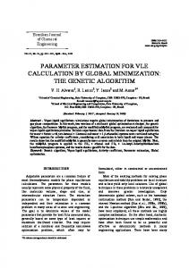
affects the smoothness of the process, as shown in the examples provided – for the 2-dimensional case – by Figures 1-3.

Let

A be any bounded set of R + and let a = min(A ) a  A , the set {X(at)} of the

and A= max(A ) . For any

a-lagged rescaled process is considered. Denoted by  the k-dimensional distribution of X and setting X a   X (at1 ), X (at2 ),..., X (atk ) , equality (1) becomes

Fig. 1. Surrogated fBm with parameter H = 0.25.

 x ( a )  x    a H0 X (1)  x  , x  R k

(5)

When X(t) is H0-self-similar, one has  a H X ( a )  x   Pr  a  H X (at1 )  x1 ,..., a  H X (atk )  xk  





 Pr a H0  H X (t1 )  x1 ,..., a H0  H X (tk )  xk    a H0 H t (1)  x  





 Pr X (t1 )  a H  H0 x1 ,..., X (tk )  a H  H0 xk 



  t (1) a

H  H0



x .



Fig. 2. Surrogated fBm with parameter H = 0.50.

Therefore, denoted by  H   a H x ( a )  x  , a  A

 x  the

set of the (absolutely continuous) k-dimensional probability H distribution functions of a X (at ) , one can define as distance function  the one induced by the sup-norm





and assume as measure of the discrepancy among the rescaled distributions the diameter  of the metric space   H ,   . Namely:

 k   H   sup sup  a xR k ai ,a jA

i

H

x ( ai )

( x)   a

H j

x(a j )

( x)

(6)

For the diameter, in [18] the following three propositions are proved. Proposition 1. {X(t), tT} is H0-ss if and only if, for any

Fig. 3. Surrogated fBm with parameter H = 0.75.

The process displays smoother and smoother surfaces as H 303

International Journal of Computer Theory and Engineering, Vol. 5, No. 2, April 2013

bounded

A  R+ and any integer k,  k   H0   0 .

Proposition 2.

a) Calculate the increment process of lag a b) For each lag in a  a  A and for each H]0, 1[ calculate: b.1) The distance  a, H  between the empirical

Let {X(t), tT} be H0-ss, A  a and

X  0 ( x  0 ). Then  k   H  is non-increasing for H  H0 and non-decreasing for H  H0. Proposition 3. Let {X(t), tT} be H0-ss, x  0 ( x  0 ) and

cumulative distribution of lag a and a b.2) Hˆ 0 (a)  arg min  a, H 

let  Ai i1,..,n be a sequence of sets such that a p  a q and

H

c) Estimate the self-similar parameter Hˆ 0 averaging on

A p  Aq for p  q . Then, with respect to the sequence  Ai  , the diameter  k   H  is: (i) non-decreasing if H  H0;

a the values Hˆ 0 ( a ) ; 3) Repeat step 1) for each dimension. Applying the algorithm to the three surrogated fBm’s of Figures 1-3, one gets the surfaces of Figures 5-7. Notice that the global minimum corresponds to the values of H0 used to simulated the series. The main problem of the above algorithm resides in the processing times required for analysing the non trivial case of k > 1 dimensions. In order to speed up the estimation procedure, we improved the algorithm as follows. Improved algorithm. 4) Fix a dimension of B. 5) For every path: a) Calculate the increment process of lag 1 b) For lags a and A and for each H]0, 1[ calculate: b.1) The distances  (a, H ) and  ( A, H ) between

(ii) an identically zero function if H = H0. Proposition 1 basically states the uniqueness of the self-similarity parameter in terms of the diameter  k   H  . Proposition 2 provides a necessary condition of self-similarity, requiring the diameter to be a monotone function of H (non increasing for H  H0 and non decreasing for H  H0). Finally, Proposition 3 states that the diameter is monotone also with respect to an increasing sequence of lags. Exploiting the three propositions, one can test for self-similarity simply by estimating the minimum of the function with respect to H, once a minimal and a maximal lag have been fixed. Further propositions are deduced in order to assess the statistical significance of  k by the well-known Kolmogorov-Smirnov test, but here we just want to focus on the estimation of H 0  arg min  k .

The empirical cumulative distribution of lag 1 and, respectively, lags a and A ;

H

Fig. 4 displays an application of the measure (6) to a one-dimensional fractional Brownian motion simulated with parameter H0 = 0.6 and setting a  1 and A  2,..., 20 . As

b.2) Hˆ 0 (a)  arg min  a, H , Hˆ 0 ( A)  arg min   A, H  ; H

H

c) Denoted by H m  min{Hˆ 0 (a), Hˆ 0 ( A)}

stated by Proposition 3, when H  H0, the diameter increases with both H  H0 and A .

and

H M  max{Hˆ 0 (a), Hˆ 0 ( A)}, fix   0 and





consider the interval I  H m   , H M   ;

III. THE ALGORITHM

6) For each lag in a  a  A and for each HI calculate:

Generally, once a k-dimensional fBm B has been simulated, the method above described can be implemented as follows

b.1) The distance  a, H  between the empirical cumulative distribution of lag a and a b.2) Hˆ 0 (a)  arg min  a, H  H

7) Estimate the self-similar parameter Hˆ 0 averaging on a the values Hˆ 0 ( a ) ; 8) Repeat step 1) for each dimension.

Fig. 4. Self-similarity parameter estimation.

Algorithm 1) Fix a dimension of B. 2) For every path:  The simulations were obtained by FracLab® using the improved Wood and Chan algorithm [21].

Fig. 5. Self-similarity parameter estimation (H=0.25).

304

International Journal of Computer Theory and Engineering, Vol. 5, No. 2, April 2013

with CPU Intel(R) XEON(TM) 3,40 GHz (two processors) and RAM 8.00 GB, with operating system environment Windows XP Professional 64 bit.

IV. CONCLUSION An algorithm is presented that significantly improves the estimation times for a self-similar process in the general case of k-dimension. Further work could to be carried out about the optimal (in a numerical sense) set A and the tolerance parameter .

Fig. 6. Self-similarity parameter estimation (H=0.50).

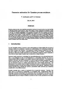
Fig. 8. Time consumption.

ACKNOWLEDGMENT Fig. 7. Self-similarity parameter estimation (H=0.75).

The above algorithm is very simple. It is composed by a pre-estimation (step 2) and an estimation (steps 3-4). The pre-estimation basically restricts to the set I the candidate self-similarity parameters H’s for which the test is run. As the maximal variation in terms of the diameter (but also in terms of the corresponding abscissae, due to numerical approximations) occurs in correspondence of the extremal lags, we first calculate the diameter for the minimal and the maximal lags. The points of minimum serve to define the set I, which is generally smaller than the whole domain [0, 1]. This significantly reduces the processing times, as shown in Table 1 and Figure 8, which reproduce the times in seconds required by the two algorithms for different sample sizes. Clearly, the time needed – independent on H – strongly depends on the set A . In our simulations we assumed as a rule of thumb A  1, 2,..., 20 , which seems a good trade-off between the accuracy of the estimation and the processing time. The tolerance parameter  was set to 0.1. TABLE I: TIME CONSUMPTION (IN SECONDS). Process length

Not improved

Improved

Ratio

256

1,793

315

17.57%

512

4,346

820

18.87%

1024

12,951

2183

16.86%

2048

38,271

6879

17.97%

The calculations were perfomed in MatLab environment (MatLab 7.9.0.529 r.2009b) on a HP Workstation XW6200 305

The authors wish to thank the Computer Lab L.I.S.A., operating at Department of Economics of University of Cassino, for supplying the software and the hardware used in this work. REFERENCES M. Á. Serrano, D. Krioukov, and M. Boguñá, “Self-similarity of complex networks and hidden metric spaces,” Phys. Rev. Lett., Feb. 2008. [2] W. Willinger, M. S. Taqqu, W. E. Leland, and D. V. Wilson, “Self-similarity in high speed packet traffic: Analysis and modelisation of ethernet traffic measurements,” Statist. Sci., vol. 10, no. 1, pp. 67-85, 1995. [3] M. S. Taqqu, W. Willinger, and R. Sherman, “Proof of a fundamental result in self-similar traffic modeling,” ACM SIGCOMM Computer Communication Review, vol. 27, no. 2, pp. 5-23, 1997. [4] Y. R. Lin, H. Sundaram, Y. Chi, J. Tatemura, and B. L. Tseng, “Detecting splogs via temporal dynamics using self-similarity analysis,” ACM Transactions on the Web, vol. 2, no.1, 2008. [5] S. Dill, R. Kumar, K. S. Mccurley, S. Rajagopalan, D. Sivakumar, and A. Tomkins, “Self-similarity in the web,” ACM Transactions on Internet Technology, vol. 2, no. 3, 2008. [6] N. Vladimirova and M. Chertkov, “Self-similarity and universality in rayleigh-taylor, boussinesq turbulence,” Physics of Fluids, vol. 21, no. 1, 2008. [7] N. S.-N. Lam and D. A. Quattrochi, “On the issues of scale, resolution, and fractal analysis in the mapping sciences,” Professional Geographer, vol. 44, no. 1, pp. 88-98, 1989. [8] B. P. Buttenfield, “Scale-dependence and self-similarity in cartographic lines,” Cartographica, vol. 26, no. 1, pp. 79-100, 1989. [9] W. Willinger, M. S. Taqqu, and V. Teverovsky, “Long range dependence and stock returns,” Finance and Stochastic., vol. 3, pp. 1-13, 1999. [10] S. Bianchi and A. Pianese, “Scaling laws in stock markets. An analysis of prices and volumes,” in Mathematical and Statistical Methods in Finance, Ed. Perna, Sibillo, Springer, 2008, pp. 35-42. [11] S. Bianchi and A. Pianese, “Multiscaling in the distribution of the exchange rates,” WSEAS Transactions on Mathematics, vol. 6, pp. 354-360, 2006. [1]

International Journal of Computer Theory and Engineering, Vol. 5, No. 2, April 2013 [12] X. Zhaoxia and G. Ramazan, “Scaling, self-similarity and multifractality in FX markets,” Physica A, vol. 323, pp. 578-590, 2003. [13] F. Pontiggia, G. Colombo, C. Micheletti, and H. Orland, “Anharmonicity and self-similarity of the free energy landscape of protein G,” Phys. Rev. Lett., vol. 98, no. 4, 2007. [14] E. Shechtman and M. Irani, “Matching local self-similarities across images and videos,” Presented at the IEEE Conference on Computer Vision and Pattern Recognition, 2007. [15] J. M. Dudley, C. Finot, D. J. Richardson, and G. Millot, “Self-similarity in ultrafast nonlinear optics,” Nature Physics, vol. 3, pp. 597-603, 2007. [16] S. Stoev, V. Pipiras, and M. S. Taqqu, “Estimation of the self-similarity parameter in linear fractional stable motion,” Signal Processing, vol. 82, no. 12, pp. 1873-1901, 2002. [17] P. Doukhan, G. Oppenheim, and M. S. Taqqu, “Theory and Applications of Long-Range Dependence,” Ed. Birkhäuser, Boston, 2003. [18] S. Bianchi, “A new distribution-based test of self-similarity,” Fractals, vol. 3, pp. 331-346, 2004. [19] J. W. Lamperti, “Semi-stable stochastic processes,” Transactions of the American Mathematical Society, vol. 104, pp. 62-78, 1962. [20] P. Embrechts and M. Maejima, Selfsimilar Processes, Ed. Princeton University Press, Princeton, 2002. [21] B. Mandelbrot and J. V. Ness, “Fractional brownian motions, fractional noises and applications,” SIAM Review, vol. 10, no. 4, pp. 422-437, 1968. [22] A. T. A. Wood and G. Chan, “Simulation of stationary gaussian process in [0, 1]d ,” Journal of Computational and Graphical Statistics, vol. 3, no. 4, pp. 409-432, 1994.

about sixty research papers concerning the modeling of financial time series by (multi)fractional and self-similar stochastic processes. His current research interests concern market’s efficiency and behavioral finance in the light of the arbitrage principle. Prof. Bianchi is a member of the AMASES (Association of Applied Mathematics for Economic and Social Sciences).

Anna Maria Palazzo was born in Pontecorvo on 7th February 1961. She was graduated in Economics from University of Rome “La Sapienza” (Italy) in 1986. She taught Insurance Financial Management and Actuarial Science at the Faculty of Economics, University of Cassino, where she is now aggregate professor of Life Insurance. About this topic she is author of several papers and conference presentations. Her research interests mainly concern pension funds and insurance portfolios and healthcare. Alexandre Pantanella was born in Aigle (Switzerland) on 2nd December 1975. He graduated in Mechanical Engineering from University of Cassino (Italy) in 2003 and earned his Ph.D. in Mathematics for Economics and Finance from University of Rome “La Sapienza” (Italy) in 2009. He taught Mathematics and Computer Science at the Faculty of Economics, University of Cassino and he is now adjunct professor of Mathematics at the University of Cassino. He is author of about fifteen research papers concerning financial modeling and applications of multifractional stochastic processes to the finance. His research interests concern financial time series, stochastic modeling, simulation algorithms and wavelet analysis.

Augusto Pianese was born in Isola del Liri (Italy) on 2nd July 1962. He graduated in Mathematics from University of Camerino (Italy) in 1986. He taught Mathematics and Computational methods in Applied Mathematics at the Faculty of Economics, University of Cassino and he is now Aggregate Professor of Mathematical Finance and Computer Science. From 2004 he is the Director of the Computer Lab for Advanced Scientific Applications “L.I.S.A.”. He is author of several papers focused on financial and electricity market modeling. Currently, his research concern stochastic models for financial time series with a particular look at (multi)fractional and (multi)fractal processes. Prof. Pianese is a member of the AMASES (Association of Applied Mathematics for Economic and Social Sciences).

Sergio Bianchi was born in Cassino on 25th September 1967. He was graduated in Economics from University of Cassino (Italy) in 1991 and earned his Ph.D. in Actuarial and Financial Science from University of Rome “La Sapienza” (Italy) in 1997. He taught Mathematics and Financial Mathematics at the Gregorian Pontifical University, University of Rome “La Sapienza” and University of Sassari and he is now full professor of Mathematics and Mathematical Finance at the University of Cassino, where he also held the office of Head of Department from 2005 to 2009. From 2009 he is Rector’s Delegate for Research and Benchmarking. He is author of

306