The ground truth tra- jectory and landmark positions are .... More recently, Brookshire and Teller [8] have carried out a formal observability analysis in order to ...
Self-supervised Calibration for Robotic Systems Jérôme Maye, Paul Furgale, and Roland Siegwart Autonomous Systems Lab, ETH Zurich, Switzerland email: {jerome.maye, paul.furgale, roland.siegwart}@mavt.ethz.ch
I. Introduction Every robotic system has some set of parameters—scale factors, sensor locations, link lengths, etc.—that are needed for state estimation, planning, and control. Despite best efforts during construction, some parameters will change over the lifetime of a robot due to normal wear and tear. In the best case, incorrect parameter values degrade performance. In the worst case, they cause critical safety issues. We are interested in developing automated systems that are capable of robust long-term deployment in the hands of non-experts, so the automatic identification and update of these parameter values is highly important. As an example, consider a camera-based collision avoidance system intended for deployment in a consumer automobile. For the vehicle to be able to avoid collisions, the pose of each camera with respect to the vehicle coordinate system must be known precisely so that obstacle positions can be transformed from camera coordinates into vehicle coordinates. However, a consumer vehicle will have no access to special calibration hardware or expert data analysis. In such a scenario, the vehicle must be capable of selfsupervised recalibration. This problem is inherently difficult for a number of reasons that we will briefly discuss here. 1) Parameters change over time—although the vehicle may be factory calibrated, the transformations can change slowly over time due to vibration, thermal expansion, loose parts, or any number of other common problems that follow from normal usage. 2) Parameters must be inferred from the data—as the cameras may be installed in different places on the
40
35
30
25 y [m]
Abstract— We present a generic algorithm for self calibration of robotic systems that utilizes two key innovations. First, it uses information theoretic measures to automatically identify and store novel measurement sequences. This keeps the computation tractable by discarding redundant information and allows the system to build a sparse but complete calibration dataset from data collected at different times. Second, as the full observability of the calibration parameters may not be guaranteed for an arbitrary measurement sequence, the algorithm detects and locks unobservable directions in parameter space using a truncated QR decomposition of the Gauss-Newton system. The result is an algorithm that listens to an incoming sensor stream, builds a minimal set of data for estimating the calibration parameters, and updates parameters as they become observable, leaving the others locked at their initial guess. Through an extensive set of simulated and real-world experiments, we demonstrate that our method outperforms state-of-the-art algorithms in terms of stability, accuracy, and computational efficiency.
20
15
10
5
0 −5
0
5
10
15
20
25
30
35
40
x [m]
Fig. 1. Exemplary output of our calibration algorithm. The ground truth trajectory and landmark positions are shown in green, their respective estimates in blue, and the integrated odometry path in red. An information theoretic measure is used to automatically identify and store novel measurement sequences (shown in blue), discarding redundant information and building a sparse but complete calibration dataset from data collected at different times.
vehicle, their pose cannot be measured directly. Instead, the transformations must be inferred from the data produced by the full system. However, this is only possible if the motion of the vehicle renders the parameters observable1 . 3) Normal operation may result in unobservable directions in parameter space—unfortunately, for this and many other practical problems normal operation may not render all directions in parameters space observable. In this example, when two cameras do not share an overlapping field of view, planar motion renders the calibration problem degenerate2 ; the transformation between cameras only becomes observable under general 3D motion. 4) Unobservable directions in parameter space may appear observable in the presence of noise—even if our hypothetical car is piloted only on a plane (a degenerate case), noise in the measurements can make unobservable parameters appear observable. We call these parameters numerically unobservable to mirror the related concept of numerically rank-deficient matrices. Existing algorithms for self calibration generally handle issues (1) and (2). Issue (3) is dealt with by designing experiments that guarantee all parameters become observable. To the best of our knowledge, no published self-calibration 1 Informally, observability means that the parameters can be inferred from some local batch of measurement data [1] 2 See [2] for a handy table of degenerate cases or [3] for a more theoretical analysis.
algorithm is able to cope with issue (4). Therefore, unless we plan to require all vehicle owners to outfit their parking places with calibration patterns or regularly drive off-road, new advances for online system calibration are required. In this paper, we propose an algorithm to deal with all of these difficulties. Our approach exploits the algebraic links between the Gauss-Newton algorithm, the Fisher Information Matrix, and nonlinear observability analysis to automatically detect directions in parameter space that are numerically unobservable and avoid updating our parameters in these directions; at any given time, directions in the parameter space that are observable will be updated based on the latest information, while unobservable directions will remain at their initial guess. Novel sets of measurements are detected using a mutual information test, and added to a working set that is used to estimate the parameters. The result is an algorithm that listens to an incoming stream of data, automatically accumulating a batch of data that may be used to calibrate a full robot system. The only requirements are that (i) the parameters are theoretically observable given some ideal set of data, (ii) it is possible to implement a batch Gauss-Newton estimator for the system state and calibration parameters based on a set of measurements, and (iii) we have some reasonable initial guess for the calibration parameters (e.g. from factory calibration). Fig. 1 shows a typical calibration run of our algorithm. The remainder of the paper is structured as follows. Section II will give a brief overview over related approaches. Section III is dedicated to the mathematical grounding of our method. Section IV demonstrates the validity of our approach through extensive experiments and evaluation. Section V will conclude the paper. II. Related Work The problem of sensor calibration has been a recurring one in the history of robotics and computer vision. Thereby, it has been addressed using a variety of sensor setups and algorithms. A calibration process may involve recovering intrinsic, e.g. focal length for a camera, and extrinsic parameters, i.e. the rigid transformation between the sensor’s coordinate system and a reference coordinate system. For the former, one could devise a naive approach where the parameters are accurately determined during the manufacturing process. Similarly, the transformation could be retrieved by means of some measuring instrument. However, the disadvantages of such purely engineered methods are manifold. Apart from their impracticality, it can be nearly impossible to reach a satisfying accuracy and thus hinder the proper use of the sensor in a robotic system. Furthermore, external factors such as temperature variations or mechanical shocks may seriously bias a factory calibration. Therefore, much efforts have been dedicated over the years to develop algorithms for calibration of systems in the field. The use of a known calibration pattern such as a checkerboard coupled with nonlinear regression has become the most popular method in computer vision during the last decade. It has been deployed both for intrinsic camera calibration [4]
and extrinsic calibration between heterogeneous sensors [5]. While being relatively efficient, this procedure still requires expert knowledge to reach a good level of accuracy. It can also be quite inconvenient on a mobile platform requiring frequent recalibration. In an effort to automate the process in the context of mobile robotics, several authors have included the calibration problem in a state-space estimation framework, either with filtering [6] or smoothing [7] techniques. Filtering techniques based on the Kalman filter are appealing due to their inherently online nature. However, in case of nonlinear systems, smoothing techniques based on iterative optimization are usually superior in terms of accuracy. While building on this latter method, our approach attempts to reduce its computational load and copes with degenerate cases. More recently, Brookshire and Teller [8] have carried out a formal observability analysis in order to identify degenerate paths of the calibration run. In contrast to the method presented in this paper, their approach still expects that the robot travels along non-degenerate paths. A last class of methods relies on an energy function to be minimized. For instance, Levinson and Thrun [9] have defined an energy function based on surfaces and Sheehan et al. [10] on an information theoretic quantity measuring point cloud quality. To the best of the authors’ knowledge, little research has been devoted to efficiently deal with degenerate cases frequently occurring during calibration. The majority of the authors indeed assumes that their optimization routine runs on well-behaved data. As demonstrated in the next sections, this can be a critical point in real-world scenarios. In contrast, our approach does not require any of these assumptions and is suitable for online, autonomous, and long-term operations on various platforms and sensors. III. Model In this section, we will first state our problem in a probabilistic manner and present the mathematical groundings of our method. A practical algorithmic sketch will conclude the presentation. A. Problem Formulation In the following, we borrow the formalism of the probabilistic discrete-time Simultaneous Localization and Mapping (SLAM) model [11]. For the sake of clarity, we consider here a robot with a single sensor observing a known number of landmarks at each timestep. Furthermore, we assume the correspondences between sensor’s measurements and landmarks are known. While this latter assumption involves data association techniques which go beyond the scope of this paper, the extension to multiple sensors is straightforward. Let X = {x0:K } be a set of latent random variables (LRV) representing robot states up to timestep K, U = {u1:K } a set of observable random variables (ORV) representing measured control inputs, L = {ℓ1:N } a set of LRV representing N landmark positions, Z = {z11:N :K1:N } a set of ORV representing K × N landmark measurements, and Θ an LRV representing
the calibration parameters of the robot’s sensor. The goal of the calibration procedure is to compute the posterior marginal distribution of Θ given all the measurements up to timestep K, Z p(Θ | U, Z) = p(Θ, X, L | U, Z). (1) X,L
Following [11], the full joint posterior on the right-hand side of (1) may further be factorized into
p(Θ, X, L | U, Z) ∝ K N K Y Y Y p(Θ, x0 , L) p(xk | xk−1 , uk ) p(zki | xk , ℓi , Θ). (2) k=1 i=1
k=1
We may then approximate (2) with a normal distribution whose mean, µΘXL , and covariance, ΣΘXL , have to be estimated. To this end, we first derive a Maximum a Posteriori (MAP) estimator for the mean, µˆ ΘXL = arg max p(Θ, X, L | U, Z) Θ,X,L
= arg min − log p(Θ, X, L | U, Z).
(3)
Θ,X,L
When setting the prior p(Θ, x0 , L) to a uniform distribution, (3) becomes a Maximum Likelihood (ML) estimator. We shall further refine our problem by defining motion and observation models, xk = h(xk−1 , uk , wk ), zki = g(xk , ℓi , Θ, nk ),
(4)
where wk ∼ N(0, Wk ), and nk ∼ N(0, Nk )
(5)
are normally distributed process and observation noise variables, with known covariance Wk and Nk . Although, the functions h(·) and g(·) might be nonlinear in their parameters, we can approximate p(xk | xk−1 , uk ) and p(zki | xk , ℓi , Θ) as normal distributions through linearization. B. Least Squares Solution In case of linear motion and observation models, there exists a closed-form solution to (3) based on the least squares method due to the normally distributed noise variables. In the other case, one can resort to nonlinear least squares methods that iteratively solve a linearized version of the problem. In the following, we employ the Gauss-Newton algorithm [12] for this purpose. From (3) and the approximation that the densities involved are normal, we can turn the MAP problem into the minimization of a sum of squared error terms. Nonlinear optimization techniques start with an initial guess, µˆ ΘXL , and refine it iteratively with δµˆ ΘXL until convergence. δµˆ ΘXL is chosen in such a way that it minimizes a quadratic approximation of the objective function around µˆ ΘXL . Gauss-Newton method
only requires the stacked Jacobian matrix of the error terms, H. In block matrix form, the update takes the form (HT T−1 H)δµˆ ΘXL = −HT T−1 e(µˆ ΘXL ),
(6)
where T, the error covariance matrix, is built from diagonal blocks of Wk and Nk , and e(µˆ ΘXL ) is the error evaluated at the current estimate µˆ ΘXL . At convergence of the algorithm to the estimate µˆ ΘXL , the quantity HT T−1 H is the Fisher Information Matrix (FIM) and the inverse of the estimate covariance matrix, Σˆ ΘXL . If we let T−1 = LT L be the Cholesky decomposition of the error covariance matrix, (6) can be rewritten as (LH)T (LH)δµˆ ΘXL = −(LH)T Le(µˆ ΘXL ),
(7)
which we can recognize as the normal equations of the linear system (LH)δµˆ ΘXL = −Le(µˆ ΘXL ).
(8)
Thus, instead of solving (6), we can take advantage of matrix decompositions to solve (8) directly. Not only can this be more computationally efficient, the use of a rank-revealing decomposition allows the estimation of the numerical rank of the FIM, and consequently (as described below) provides information about the numerical observability of the parameters for a given batch of data. Let LH be of size m × n with the following thin3 Singular Value Decomposition (SVD) decomposition [13], LH = Un Sn VTn ,
(9)
where Un is an m × n matrix with orthogonal columns, Sn = diag(σ1 , · · · , σn ), Vn is an n × n matrix with orthogonal columns, and σi are the singular values of LH. From (9) and using the orthogonality of Un and Vn , we can solve (6) as V D) T = −Vn S−1 ˆ ΘXL ). δµˆ (S n Un Le(µ ΘXL
(10)
Although useful for illustrating the concepts of our approach, the SVD decomposition can be computationally demanding for large matrices. In practice, we therefore use the thin QR decomposition [13] of LH, LHΠ = Qn Rn ,
(11)
where Π is a permutation matrix, Qn an m × n matrix with orthogonal columns, and Rn an n×n upper triangular matrix. In standard QR decomposition, Π is the identity matrix, otherwise it reflects column pivoting. From (11) and using the orthogonality of Qn , (6) can be expressed as Rn ΠT δµˆ (QR) = −QTn Le(µˆ ΘXL ), ΘXL
(12)
which, due the upper triangular form of Rn , can be easily solved by back substitution. 3 Only the first n out of m columns of U are computed in a thin SVD decomposition.
The Rn matrix can also be used to compute the FIM and its inverse, the estimate covariance, Σˆ ΘXL . If we drop the permutation matrix for clarity, the FIM simply becomes RTn Rn and there exists an efficient algorithm [14] for recovering any elements of the covariance estimate without inverting the whole FIM. At the convergence of the Gauss-Newton optimization, we are thus left with the estimates µˆ ΘXL and Σˆ ΘXL of the normal distribution p(Θ, X, L | U, Z). In order to solve (1), we can employ the marginalization property of normal distributions [15]. If we express the estimates in the partitioned form,
µˆ ΘXL
µˆ X = µˆ L , µˆ Θ
Σˆ ΘXL
ˆ ΣXX = Σˆ LX ˆ ΣΘX
Σˆ XL Σˆ LL Σˆ ΘL
Σˆ XΘ Σˆ LΘ , Σˆ ΘΘ
(13)
then p(Θ | U, Z) ∼ N(µˆ Θ , Σˆ ΘΘ ). We can thus extract µˆ Θ from µˆ ΘXL very efficiently, and by placing Θ to the right of the Jacobian matrix H and using [14], Σˆ ΘΘ can be computed in O(l), where l = card(Θ). C. Truncated SVD and QR Solutions There exists a solution to (6) iff the FIM is invertible, i.e., it is full rank4 . Jauffret [16] clearly articulates the link between the rank of the FIM and observability of the parameters being estimated. In the context of calibration, a singular FIM corresponds to some unobservable directions in the parameter space given the current set of observations. Classical observability analysis, for example the widely used method of Hermann and Krener [17] (c.f. [18] or [19]), proves what we will call structural observability—that there exists some dataset for which the parameters are observable—it does not guarantee that the parameters are observable for any dataset. In real-world scenarios, where data is contaminated by noise, the FIM might appear to be full rank although it is actually rank-deficient. We can illustrate this with the matrix 0.9999 1.9999 3.0014 A = 4.0007 5.0015 6.0007 . (14) 6.9998 8.0014 8.9988
Although A is technically full rank, it was constructed from a structurally rank-deficient matrix (the second row is a linear combination of the first and the last row) with added Gaussian noise. Using SVD decomposition, we can identify a numerically rank-deficient matrix by analyzing its singular values [20] and consequently the numerical observability of the system [21] [22]. The numerical rank r of a matrix is defined as the index of its smallest singular value σr larger than a user-defined tolerance ǫ, i.e., r = arg max σi ≥ ǫ. i
(15)
4 The rank of a matrix is the maximum number of linearly independent column or row vectors. A matrix with m rows and n columns has full rank when its rank is equal to min(m, n).
For example, the singular values of A are approximately 16.8, 1.1, and 0.0001. From (10), we can see that if some of the σi are close to zero, i.e. r < n, the update vector V D) δµˆ (S will be large (scaled by 1/σi ) and sometimes lead to ΘXL a divergence of the solution. In order to cope with this issue, we can approximate LH with a lower-rank matrix yielding the Truncated SVD (TSVD) [23] solution, (T S V D) T δµˆ ΘXL = −Vr S−1 ˆ ΘXL ), r Ur Le(µ
(16)
with Ur an m × r matrix, Sr = diag(σ1 , · · · , σr ), Vr an n × r matrix. It is worth noting that TSVD applies a sharp filter to the system, whereas regularization methods such as Tikhonov or ridge regression work as a smooth filter. As shown in [24], it nevertheless produces similar results at lower computational costs when the matrix has a well-determined numerical rank, i.e., a clearly defined jump in the singular values spectrum. A similar approach can be derived using rank-revealing QR decomposition [25] yielding the Truncated QR (TQR) method [26]. The strategy is to apply QR factorization with column pivoting in order to reveal the rank and to apply a cutoff on the diagonal of the R matrix. It can further be noted that the Q matrix need not be explicitly constructed, but instead returned in the form of Householder reflections that can be applied to the right-hand side of the linear system. According to the discussion in [13], column scaling may improve the conditioning of the system, i.e. the ratio between the largest and the smallest singular value, and hence the stability of the solution. Within our framework, scaling is also relevant for merging quantities with miscellaneous magnitudes and helps in setting a rank tolerance ǫ that is widely applicable. We define the scaling matrix as ) ( 1 1 , (17) ,··· , G = diag ||LH(:, 1)|| ||LH(:, n)|| where ||·|| denotes the column vector norm and H(:, i) the i-th column of H, and compute a solution to the scaled system, LHGδµˆ (s) = −Le(µˆ ΘXL ). ΘXL
(18)
The unscaled solution is finally expressed as Gδµˆ (s) . ΘXL D. Selecting Informative Measurements Since we are mainly interested in calibrating our sensor and thus in the posterior p(Θ | U, Z), we do not need to consider all the measurements. Let us define a partition of the measurements D1 = {u1:i , z11:N :i1:N } and D2 = {ui+1:K , zi+11:N :K1:N } with i < K. Using information theory, we can quantify the information gain when estimating Θ with D1 alone or with D1 ∪ D2 . The mutual information (MI) [27] between two random variables X and Y is defined as Z Z p(x, y) I(X; Y) = p(x, y) log , (19) p(x)p(y) X Y where p(x, y) is the joint density of X and Y, and p(x) and p(y) their marginal densities. The MI measures the amount
of information X and Y share or, in other words, quantifies the reduction of uncertainty in X when knowing Y. Before deriving the MI for our purpose, it is worth recalling another property of normal distributions [15]. If we define Θ1 = Θ | D1 and consider the joint normal distribution p(Θ1 , D2 ) with parameters µΘ1 D2 =
!
µΘ1 Σ , ΣΘ1 D2 = Θ1 Θ1 µD2 ΣD2 Θ1
!
ΣΘ1 D2 , ΣD2 D2
(20)
then p(Θ1 | D2 ) is a normal distribution with parameters µΘ1 |D2 = µΘ1 + ΣΘ1 D2 Σ−1 D2 D2 (D2 − µD2 )
ΣΘ1 |D2 = ΣΘ1 Θ1 − ΣΘ1 D2 Σ−1 D2 D2 ΣD2 Θ1 .
(21)
Furthermore, ΣΘ1 |D2 can be recognized as the Schur complement of the joint covariance matrix ΣΘ1 D2 . Following an argument of [28], the MI between Θ1 and D2 can then be computed as |ΣΘ1 Θ1 | 1 log 2 |ΣΘ1 Θ1 − ΣΘ1 D2 Σ−1 D2 D2 ΣD2 Θ1 | |Σ | 1 Θ1 Θ1 , = log 2 |ΣΘ1 |D2 |
I(Θ1 ; D2 ) =
(22)
where | · | denotes the matrix determinant and ΣΘ1 |D2 is the covariance estimate of Θ using D1 and D2 , which is computed by Gauss-Newton optimization. Thus, using (22), we can measure the amount of information D2 conveys to our current estimate Θ | D1 .
Algorithm 1: calibrateSensor() ˆ (0) , xˆ (0) , Lˆ (0) Input: Initial guesses Θ 0 Input: Motion h(·) and observation g(·) models Input: Batch size k, TQR threshold ǫ, MI threshold λ Output: µˆ Θ and Σˆ ΘΘ Din f o ← ∅ ; t←1; while calibrate do // Collecting measurements ; tinit ← t ; Dnew ← ∅ ; while t < tinit + k do xˆ (0) x(0) t ← h(ˆ t−1 , ut , 0) ; new D ← Dnew ∪ {ut , zt1:N } ; t ←t+1 ; end // TQR optimization with threshold ǫ ; µˆ ΘXL ← arg maxΘ,X,L p(Θ, X, L | Din f o , Dnew ) ; // Marginalization ; µˆ Θ ← µˆ ΘXL ; Σˆ ΘΘ ← Σˆ ΘXL ; // MI decision ; if I(Θ | Din f o ; Dnew ) > λ then Din f o ← Din f o ∪ Dnew ; Θ ∼ N(µˆ Θ , Σˆ ΘΘ ) ; end end
E. Algorithm Thus far, we have delivered a formal introduction to the probabilistic groundings of our self-supervised calibration approach. This section will be dedicated to a practical online implementation of our algorithm. The proposed calibration method is sketched in Alg. 1. Defining Din f o as the set of informative measurements at time t, we collect a measurement batch Dnew = {ut:t+k , zt1:N :t+k1:N } during k timesteps and compute p(Θ | Din f o , Dnew ) using Gauss-Newton method with TQR updates and threshold ǫ. In a second step, if I(Θ | Din f o ; Dnew ) is larger than a user-defined threshold λ, Dnew is added to Din f o and the estimate of Θ is updated. Given the structure of the model (2), the Jacobian matrix H will be sparsely populated. Therefore, in order to obtain a tractable and scalable method, we adopt sparse matrices algorithms and data structures. The memory and computational costs are then O(card(X) × card(L)). IV. Experiments In order to evaluate and validate the approach proposed in this paper, we have conducted experiments on simulated and real-world data. We shall first start with the description of the experimental conditions and then demonstrate the performance of our algorithm, along with some comparisons against existing methods.
A. Experimental Setup
Our method has been fully implemented in MATLAB and we have used the SuiteSparseQR [29] package for performing sparse matrix operations. Although our eventual goal is full, self-supervised calibration for an autonomous vehicle system with multiple heterogeneous sensors, the experiments in this paper are based on a realistic, but somewhat simplified robotic system. This allows us to precisely control the observability properties in simulation and test the behavior of our algorithm. Fig. 2 depicts our experimental setup. The platform is a differential drive mobile robot equipped with a range sensor delivering range and bearing measurements. The calibration parameters of the range sensor consist in the transformation of its coordinate system to the robot’s coordinate system. The platform is further endowed with wheel odometers outputting translational and rotational speeds. While navigating on the plane, the robot observes a known number of landmarks through its range sensor. Both the range sensor and the odometry produce data at 10 Hz. More formally, we adopt the following motion and observation models
ℓi
20
rki
15
10 y [m]
φik
ψ
δx yk
5
θk
δy
0
−5 0
5
10
15
20
25
x [m]
xk Fig. 2. Experimental setup. A 2D robot moving in a plane and observing landmarks with a range sensor providing range and bearing angle measurements. The calibration process needs to find the 2D transformation between the robot’s coordinate system and the sensor’s coordinate system.
Fig. 3. Straight path example. The green line represents the ground truth path, the red line the integrated odometry path, the green circles the ground truth landmark positions, and the red circles the guessed landmark positions.
[bits] in our experiments. The ǫ parameter shall be discussed below. B. Simulated Data
! ! xk xk−1 cos θk−1 0 yk = yk−1 + T sin θk−1 0 vk + wk wk θk θk−1 0 1 |{z} | {z } xk
h(xk−1 ,uk ,wk )
a = xi − xk − δ x cos θk + δy sin θk b = yi − yk − δ x sin θk − δy cos θk √ ! ! rki a2 + b2 + nk , = φik atan2(b, a) − θk − ψ |{z} | {z } zki
(23)
g(xk ,ℓi ,Θ,nk )
where xk = [xk yk θk ]T denotes the robot pose at timestep k, T the sampling period, uk = [vk wk ]T the measured translational and rotational speeds, zki = [rki φik ]T the range and bearing observation of landmark i with pose ℓi = [xi yi ]T , wk ∼ N(0, Wk ) with Wk = diag(σ2v , σ2w ), nk ∼ N(0, Nk ) with Nk = diag(σ2r , σ2φ ), and Θ = [δ x δy ψ]T the range sensor’s calibration parameters. Throughout our experiments, we have used a noninformative prior p(Θ, x0 , L), i.e., a uniform distribution. The use of priors is still subject to controversial discussions [30] between Bayesian and non-Bayesian statisticians. Here, we argue that everything should come from the data itself and not from some subjective prior information that could bias the inference. Our algorithm requires only 3 free parameters, namely the rank threshold ǫ, the batch size k, and the MI threshold λ. Optimally, k should be inferred from the dynamics of the system. While a large k induces storage of uninformative measurements, a small k leads to useless runs of optimization and makes it difficult to discover informative sequences of measurements. In this setup, we have used a batch size of k = 100 (ten seconds of data). Concerning the MI threshold, a small λ will keep most of the measurements and a large λ will ignore them all. We have set this value to λ = 0.5
In our simulation environment, we can generate various paths for the robot, along with corresponding sensor measurements, and thus analyze the behavior of multiple algorithms, especially in degenerate cases. We have created an environment with N = 17 landmarks uniformly distributed on a 20m × 20m grid. We have set the noise parameters empirically to σ2v = 4.4 × 10⁻³ , σ2w = 8.2 × 10⁻² , σ2r = 9.0036 × 10⁻⁴ , and σ2φ = 6.7143 × 10⁻⁴ . The calibration parameters are fixed at δ x = 0.219 [m], δy = 0.1 [m], and ψ = π/4 [rad]. In a first effort, we want to support the claims of Sec. IIIC with a representative example. We simulated the robot driving along a straight path as shown in Fig. 3. Intuitively, the problem is structurally unobservable. Indeed, it has 5 unobservable parameters, 3 corresponding to the global pose of the map and trajectory (as no global measurements or prior are included) and 2 for the calibration offset variables δ x and δy . In the absence of noise, 5 of the singular values of the Jacobian matrix are zero up to machine precision, i.e., a structural rank deficiency. However, when noise is added, only 3 singular values remain at 0 for the same problem. From the integrated odometry path in Fig. 3, the calibration parameters appear indeed as observable and a naive algorithm without regularization will thus wrongly optimize. Fig. 4 shows the singular values in these two cases and the related concept in the QR decomposition. With our TSVD/TQR method, we can deal with this issue by setting an adequate ǫ threshold that will recover the correct rank deficiency and therefore only optimize the observable parts. The threshold is application-specific and should be a function of the system noise. Obviously, at a certain level of noise, gaps in the singular values spectrum become indistinguishable. In our setup, we have determined the threshold empirically from the scaled system (18) and set it to ǫ = 0.013. To conclude this section on simulated data, we will analyze the performance of different algorithms, namely an Extended
4 0.25
0.2
0.2
0.15
0.15
0.1
0.1
0.05
0.05
0
0 0
10
20
30
40
50
60
70
80
90
100
0.9 0.8 0.7 0.6 0.5 0.4 0.3 0.2 0.1 0
3
2
1
0
10
20
30
40
50
60
70
80
90
100
0.9 0.8 0.7 0.6 0.5 0.4 0.3 0.2 0.1 0 0
10
20
30
40
50
60
70
80
90
100
y [m]
0.25
0
−1
−2
−3
−4 −2 0
10
20
30
40
50
60
70
80
90
0
2
4
6
100
Fig. 4. Straight path example analysis. The first column shows the singular values and the diagonal elements of the R matrix from the QR decomposition in the noise-free case, and the second column in the noisy case. Only the 100 lower values from the scaled system (18) are plotted for visualization purpose.
Kalman Filter (EKF) similar to [6], a standard batch nonlinear least squares (LS) method without regularization [7], and our TQR-MI approach, on a sine wave path with varying amplitude such that the offset parameters range from unobservable (straight path or zero amplitude) to fully observable (higher amplitude). To get significant statistical results, we have repeated the experiment 100 times with the same initial (0) (0) conditions (δ(0) = 0.8 [rad]) x = 0.23 [m], δy = 0.11 [m], ψ and amplitudes from 0 [m] to 5 [m] with steps of 0.5 [m] over 5000 timesteps (500 [s] of data). Fig. 5 displays the result of this experiment. At amplitude 0, we clearly witness that the LS and EKF estimators fail to yield reasonable offset parameters. With our TQR-MI method, these parameters remain at their initial guess until an amplitude of 1 and only the angle gets optimized. As the amplitude grows, our method becomes comparable to the LS estimator, while using fewer measurements. In these experiments, the EKF is fed by a vague initial prior and exhibits instability in case of unobservability. A more concentrated prior would improve the results at the cost of introducing potential bias. C. Real-world Data In order to validate our method on real-world data, we have used the “Lost in the Woods Dataset” provided with the courtesy of Tim Barfoot [31]. This dataset contains approximately 20 minutes of a robot driving amongst a forest of tubes which serve as landmarks. The ground truth comes from a motion capture system that tracks robot motion and tube locations. For the calibration parameters, we have only access to δ x = 0.219 [m] that was roughly measured with a tape. We assume the others are implicitly set to 0 (δy = 0 [m] and ψ = 0 [rad]). Fig. 6 displays the qualitative result of our algorithm. Using only 10% of the measurements, we could recover accurate landmark positions, robot poses, and calibration parameters. For visualization, estimated landmarks and poses have been aligned to the ground truth using the algorithm from [32]. Since the ground truth calibration parameters are inaccurate, Tab. I compares our method against a standard least squares (LS) estimator that exploits all the measurements.
8
10
12
14
x [m]
Fig. 6. Application of our algorithm on the “Lost in the Woods dataset”. The green line represents the ground truth path, the red line the integrated odometry path, the green crosses the ground truth landmark positions, the blue points the estimated landmark positions, and the blue crosses the estimated robot poses. Our MI selection scheme picks only 10% of the measurements for the optimization. TABLE I Comparison of a standard least squares estimator and our method on the “Lost in the Woods dataset”.
δˆ x [m] δˆ y [m] ψˆ [rad] ˆΣδ x [m2 ] Σˆ δy [m2 ] ˆΣψ [rad2 ] K
LS
TQR-MI
0.2357
0.2344
0.0031
0.0087
0.0804
0.0754
0.0908 × 10⁻⁵
0.1903 × 10⁻⁴
0.0286 × 10⁻⁵
0.0582 × 10⁻⁴
0.3917 × 10⁻⁵ 12609
0.7243 × 10⁻⁴ 1209
Our TQR-MI algorithm performs the optimization with K = 1209 out of 12609 timesteps. Although the calibration parameters are the same magnitude, the higher variances stem from the fewer number of considered measurements. V. Conclusion In this paper, we have presented a novel approach to the automatic calibration of mobile robot sensors. We have included the calibration parameters in a SLAM formulation and computed an MAP estimator using a Gauss-Newton algorithm. To cope with unobservability, we have employed truncated QR decomposition as a regularization method. For long-term and online operations, we have devised a mutual information selection scheme that solely captures informative measurements relevant to the calibration. Our algorithm has been thoroughly tested and validated through extensive simulated and real-world experiments on a 2D robot equipped with a laser range finder (LRF). In the near future, we will consider the self calibration of multiple sensors (cameras, 3D/2D LRF, GPS/INS system, . . . ) mounted on an autonomous car and a C++ implementation. From a research point of view, we would like to further automate the selection of the free parameters. Lastly, we want to detect stepwise changes in the calibration parameters in order to trigger recalibration in case of mechanical shocks.
0.5
δx RMS [m]
0.4 0.3 0.2 0.1 0 0.5
δy RMS [m]
0.4 0.3 0.2 0.1 0 0.5
ψ RMS [rad]
0.4 0.3 0.2 0.1 0 0
0.5
1
1.5
2
2.5
3
3.5
4
4.5
5
Amplitude [m]
Fig. 5. Comparison of a least squares (red), EKF (blue), and our TQR-MI (green) estimator on a sine wave path of 5000 timesteps with varying amplitudes (0 to 5 [m] with steps of 0.5 [m]). For each amplitude and method, 100 simulations are performed and the RMS errors of the computed calibration parameters (δ x , δy , and ψ) are reported. The plots are scaled to show the behavior of the algorithms near RMS = 0.
Acknowledgment This work has partly been supported by the EC under FP7-269916-V-Charge. References [1] A. H. Jazwinski, Stochastic Processes and Filtering Theory. Academic Press, 1970. [2] P. Lébraly, E. Royer, O. Ait-Aider, and M. Dhome, “Calibration of non-overlapping cameras - application to vision-based robotics,” in Proc. 21st British Machine Vision Conf. (BMVC), 2010. [3] J.-H. Kim and M. J. Chung, “Absolute motion and structure from stereo image sequences without stereo correspondence and analysis of degenerate cases,” Pattern Recognition, vol. 39, pp. 1649–1661, 2006. [4] P. F. Sturm and S. J. Maybank, “On plane-based camera calibration: A general algorithm, singularities, applications,” in Proc. 12th IEEE Conf. Comput. Vision and Pattern Recognition (CVPR), 1999. [5] Q. Zhang and R. Pless, “Extrinsic calibration of a camera and laser range finder (improves camera calibration),” in Proc. IEEE/RSJ Int. Conf. Intell. Robots Syst. (IROS), 2004. [6] A. Martinelli, D. Scaramuzza, and R. Siegwart, “Automatic selfcalibration of a vision system during robot motion,” in Proc. IEEE Int. Conf. Robot. Automat. (ICRA), 2006. [7] R. Kuemmerle, G. Grisetti, and W. Burgard, “Simultaneous calibration, localization, and mapping,” in Proc. IEEE/RSJ Int. Conf. Intell. Robots Syst. (IROS), 2011. [8] J. Brookshire and S. Teller, “Extrinsic calibration from per-sensor egomotion,” in Proc. 8th Robot.: Sci. Syst. Conf. (RSS), 2012. [9] J. Levinson and S. Thrun, “Unsupervised calibration for multi-beam lasers,” in Proc. 12th Int. Symp. Experimental Robotics (ISER), 2010. [10] M. Sheehan, A. Harrison, and P. Newman, “Self-calibration for a 3D laser,” Int. J. Robot. Research (IJRR), vol. 31, pp. 675–687, 2012. [11] H. Durrant-Whyte and T. Bailey, “Simultaneous localization and mapping: Part I,” IEEE Robot. Automat. Mag. (RAM), vol. 13, pp. 99–108, 2006. [12] R. C. Aster, B. Borchers, and C. H. Thurber, Parameter Estimation and Inverse Problems. Academic Press, 2011. [13] G. H. Golub and C. F. V. Loan, Matrix Computations. The Johns Hopkins University Press, 1996. [14] M. Kaess and F. Dellaert, “Covariance recovery from a square root information matrix for data association,” Robot. Autonomous Syst. (RAS), vol. 57, pp. 1198–1210, 2009. [15] C. M. Bishop, Pattern Recognition and Machine Learning. Springer, 2006.
[16] C. Jauffret, “Observability and Fisher information matrix in nonlinear regression,” IEEE Trans. Aerosp. Electron. Syst., vol. 43, pp. 756–759, 2007. [17] R. Hermann and A. J. Krener, “Nonlinear controllability and observability,” IEEE Trans. Automat. Contr., vol. 22, pp. 728–740, 1977. [18] J. Kelly and G. S. Sukhatme, “Visual-inertial sensor fusion: Localization, mapping and sensor-to-sensor self-calibration,” Int. J. Robot. Research (IJRR), vol. 30, pp. 56–79, 2011. [19] F. M. Mirzaei and S. I. Roumeliotis, “A Kalman filter-based algorithm for IMU-camera calibration: Observability analysis and performance evaluation,” IEEE Trans. Robot., vol. 24, pp. 1143 – 1156, 2008. [20] P. C. Hansen, Rank-Deficient and Discrete Ill-Posed Problems: Numerical Aspects of Linear Inversion. Society for Industrial and Applied Mathematics (SIAM), 1998. [21] B. P. Gibbs, Advanced Kalman Filtering, Least-Squares and Modeling: A Practical Handbook. Jon Wiley & Sons, 2011. [22] L. K. Huat, Ed., Industrial Robotics: Programming, Simulation and Applications. Pro Literatur Verlag, 2006. [23] J. M. Varah, “On the numerical solution of ill-conditioned linear systems with applications to ill-posed problems,” SIAM J. Numerical Anal., vol. 10, pp. 257–267, 1973. [24] P. C. Hansen, “The truncated SVD as a method for regularization,” BIT, vol. 27, pp. 534–553, 1987. [25] Y. P. Hong and C.-T. Pan, “Rank-revealing QR factorizations and the singular value decomposition,” Mathematics of Computation, vol. 58, pp. 213–232, 1992. [26] T. Kitagawa, S. Nakata, and Y. Hosoda, “Regularization using QR factorization and the estimation of the optimal parameter,” BIT, vol. 41, pp. 1049–1058, 2001. [27] D. J. MacKay, Information Theory, Inference, and Learning Algorithms. Cambridge University Press, 2005. [28] A. J. Davison, “Active search for real-time vision,” in Proc. 10th IEEE Int. Conf. Comput. Vision (ICCV), 2005. [29] T. A. Davis, “Algorithm 915: SuiteSparseQR: Multifrontal multithreaded rank-revealing sparse QR factorization,” ACM Trans. Math. Softw., vol. 38, pp. 1–24, 2011. [30] A. Gelman, “Objections to Bayesian statistics,” Bayesian Analysis, vol. 3, pp. 445–450, 2008. [31] C. H. Tong, P. Furgale, and T. D. Barfoot, “Gaussian process GaussNewton: Non-parametric state estimation,” in Proc. 9th Conf. Comput. Robot Vision (CRV), 2012. [32] P. D. Fiore, “Efficient linear solution of exterior orientation,” IEEE Trans. Pattern Anal. Machine Intell. (PAMI), vol. 23, pp. 140–148, 2001.