Self-tuning control of non-linear systems using Gaussian process prior ...

Self-tuning control of non-linear systems using Gaussian process prior models Daniel Sbarbaro and Roderick Murray-Smith Departamento de Ingenier´ia El´ectrica, Universidad de Concepci´on, Chile. Department of Computing Science, University of Glasgow, Glasgow G12 8QQ, Scotland, UK. & Hamilton Institute, NUI Maynooth, Ireland. May 15, 2003

Abstract Gaussian Process prior models, as used in Bayesian non-parametric statistical models methodology are applied to implement a nonlinear adaptive control law. The expected value of a quadratic cost function is minimised, without ignoring the variance of the model predictions. This leads to implicit regularisation of the control signal (caution) in areas of high uncertainty. As a consequence, the controller has dual features, since it both tracks a reference signal and learns a model of the system from observed responses. The general method and its main features are illustrated on simulation examples.

1 Introduction Linear control algorithms have been successfully applied to control nonlinear systems, since they can adapt their parameters to cope the nonlinear characteristics of real systems. However, their performance degrades as the system undergo rapid and larger changes in its operating point. Several authors have proposed the use of non-linear models as a base to build nonlinear adaptive controllers. Agarwal and Seborg (Agarwal and Seborg, 1987), for instance, have proposed the use of known nonlinearities, capturing the main characteristic of the process, to design a Generalized Minimum Variance type of self-tuning controller. In many applications, however, these nonlinearities are not known, and non-linear parameterision must be used instead. A popular choice has been the use of Artificial Neural Networks for estimating the nonlinearities of the system (Narendra and Parthasarathy, 1990; Liang and ElMargahy, 1994; Chen and Khalil, 1995; Bittanti and Piroddi, 1997). All these works have adopted the certainty equivalence principle for 1

designing the controllers, where the model is used in the control law as if it were the true system. In order to improve the performance of nonlinear adaptive controllers based on a nonlinear models, the accuracy of the model predictions should also be taken into account. A common approach to consider the uncertainty in the parameters, is to add an extra term in the cost function of a Minimum Variance controller, which penalizes the uncertainty in the parameters of the nonlinear approximation (Fabri and Kadirkamanathan, 1998). Another similar approach based on the minimization of two separate cost functions, has been proposed in (Filatov et al., 1997), the first one is used to improve the parameter estimation and the second one to drive the system output to follow a given reference signal. This approach is called bicriterial and it has also be extended to deal with nonlinear systems (Sbarbaro et al., 1998). Most of these engineering applications are still based on parametric models, where the functional form is fully described by a finite number of parameters, often a linear function of the parameters. Even in the cases where flexible parametric models are used, such as neural networks, spline-based models, multiple models etc, the uncertainty is usually expressed as uncertainty of parameters (even though the parameters often have no physical interpretation), and do not take into account uncertainty about model structure, or distance of current prediction point from training data used to estimate parameters. This paper describes an approach based on Gaussian process priors, as an example of a non-parametric model with particularly nice analytic properties. This allow us to analytically obtain a control law which perfectly minimises the expected value of a quadratic cost function, which does not disregard the variance of the model prediction as an element to be minimised. This leads naturally, and automatically to a suitable combination of regularising caution in control behaviour in following the reference trajectory, depending on model accuracy. This paper expands on previous work (Murray-Smith and Sbarbaro, 2002) by making the cost function more flexible, and investigating modelling and control performance for nonlinear systems affine in control inputs. The above ideas are closely related to the work done on dual adaptive control, where the main effort has been concentrated on the analysis and design of adaptive controllers based on the use of the uncertainty associated with parameters of models with fixed structure (Wittenmark, 1995; Filatov and Unbehauen, 2000). The paper is organised as follows: section 2 describes the characteristics of non-parametric models. Section 3 introduces Gaussian Process priors. Section 4 illustrates how to design controllers based on the above representation. In section 5, we illustrate the control behaviour via simulation. Finally, some conclusions and future directions are outlined.

2

2 Non-parametric models and uncertainty prediction Non-parametric models retain the available data and perform inference conditional on the current state and local data (called ‘smoothing’ in some frameworks). As the data are used directly in prediction, unlike the parametric methods more commonly used in control contexts, non-parametric methods have advantages for off-equilibrium regions, since normally in these regions the amount of data available for identification is much smaller than that available in steady state. The uncertainty of model predictions can be made dependent on local data density, and the model complexity automatically related to the amount and distribution of available data (more complex models need more evidence to make them likely). Both aspects are very useful in sparsely-populated transient regimes. Moreover, since weaker prior assumptions are typically applied in a non-parametric model, the bias is typically less than in parametric models. Non-parametric models are also well-suited to initial data analysis and exploration, as they are powerful models of the data, with robust behaviour despite few prior structural assumptions.

3 Gaussian Process priors In a Bayesian framework the model must be based on a prior distribution over the infinite-dimensional space of functions. As illustrated in (O’Hagan, 1978), such priors can be defined as Gaussian processes. These models have attracted a great deal of interest recently, in for example reviews such as (Williams, 1998). Rasmussen (1996) showed empirically that Gaussian processes were extremely competitive with leading nonlinear identification methods on a range of benchmark examples. The further advantage that they provide analytic predictions of model uncertainty makes them very interesting for control applications. Use of GPs in a control systems context is discussed in (Murray-Smith et al., 1999; Leith et al., 2000). A variation which can include ARMA noise models is described in (Murray-Smith and Girard, 2001). k-step ahead prediction with GP’s is described in (Girard et al., 2003) and integration of prior information in the form of state or control linearisations is presented in (Solak et al., 2003). In the following, the full matrix of state and control input vectors is denoted Φ Φ, and the vector of output points is y. The discrete data of the regression model are φk = [x(t − 1) u(t − 1)] and yk = y(t). In the example used in this paper, x(t − 1) = [y(t − 1), . . . , y(t − n), u(k − 2), . . . , u(t − m)]. The given N1 data pairs used for identification are stacked in matrices Φ1 , y1 and the N2 data pairs used for prediction are Φ2 , y2 . Instead of parameterising y(t) = f (φ(t)) as a parametric model, we can place a prior directly on the space of functions where

3

f is assumed to belong. A Gaussian process represents the simplest form of prior over functions – we assume that any p points have a p-dimensional multivariate Normal distribution. We will assume zero mean, so for the case with partitioned data y1 and y2 we will have the multivariate Normal distribution (we will assume zero mean1 ),     y1 Σ1 Σ12   ∼ N (0, Σ) , Σ =  . y2 Σ21 Σ2

(1)

where Σ is the full covariance matrix, and where Σ21 = ΣT12 . Like the Gaussian distribution, the Gaussian Process is fully specified by a mean and its covariance function, so we denote the distribution GP (µ, C). The covariance function C(xi , xj ) expresses the expected covariance between yi and yj – we can therefore infer y2 ’s from constant Φ1 , y1 ’s rather than building explicit parametric models. As in the multinormal case, we can divide the joint probability into a marginal Gaussian process and a conditional Gaussian process. The marginal term gives us the likelihood of the training data, P (y1 |Φ1 ) = (2π)−

N1 2

−1

|Σ1 |− 2 e(− 2 y1 Σ1 1

1

T

y1 )

.

(2)

The conditional part of the model, which best relates to a traditional regression model is therefore the Gaussian process, which gives us the output posterior density function conditional on the training data Φ1 , y1 and the test points Φ2 , P (y2 |Φ1 , y1 , Φ2 ) =

P (y2 , y1 ) P (y1 ) T Σ−1 (y −µ ) 2 21 21

1

=

e− 2 (y2 −µ21 ) (2π)

N2 2

1

,

|Σ21 | 2

where, as in the straightforward multinormal case described earlier, µ2.1 = ΣT12 Σ−1 1 y1

(3)

Σ2.1 = Σ2 − ΣT12 Σ−1 1 Σ21 ,

(4)

so we can use y(Φ2 ) = µ21 as the expected model output, with a variance of σ(Φ2 ) = Σ21 . 1

Note, as explained in (Neal, 1997) the zero mean assumption does not mean that we expect the regression function to be spread equally

on either side of zero. If a covariance function had a large constant term the actual function could be always positive or always negative over the range of interest. The zero mean reflects or ignorance as to what that sign will be. There are good numerical computational reasons for transforming data to be zero mean.

4

3.1 The covariance function The Normal assumption may seem strangely restrictive initially, but represents a powerful tool since the model’s prior expectations can be adapted to a given application by altering the covariance function. The choice of function is only constrained in that it must always generate a non-negative definite covariance matrix for any inputs Φ, so we can represent a spectrum of systems from very local nonlinear models, to standard linear models using the same framework. The covariance function will also often be viewed as being the combination of a covariance function due to the underlying model Cm and one due to measurement noise Cn . The entries of this matrix are then: Σ1ij = Cm (Φ1i , Φ1j ; Θ) + Cn (Φ1i , Φ1j ; Θ)

(5)

where Cn () could be δij N (Φ1 ; Θ), which would be adding a noise model N to the diagonal entries of Σ1 . We discuss covariance functions for correlated noise models in (Murray-Smith and Girard, 2001). In this paper, we use a straightforward covariance function, C(xi , xj ; Θ) = v0 ρ(|xi − xj |, α) +

p X

ak xik xjk + a0 ,

k=1

so that the parameter vector Θ = [v0 , α1,..p , a0 ]T and p is the dimension of vector x . The function ρ(d) is a distance measure, which should be one at d = 0 and which should be a monotonically decreasing function of d. The one used here was 1

ρ(|xi − xj |, α) = e− 2

Pp k=1

αk (xik −xjk )2

.

(6)

The αk ’s determine how quickly the function varies in dimension k. This estimates the relative smoothness of different input dimensions, and can therefore be viewed as an automatic relevance detection (ARD) tool, which helps weight the importance of different input dimensions. Other bases which included a nonlinear transformation of x, like the RBF neural networks used in (Fabri and Kadirkamanathan, 1998), could be put into this framework. The prior associated with this covariance function states that outputs associated with φ’s closer together should have higher covariance than points further apart. Since the output is an affine function of the control input, it is reasonable to add a covariance contribution from the control inputs as an affine function as well: Cm (φi , φj ) = Cx (xi , xj ) + Caf f (φi , φj )

(7)

where Cx = Cx (xi , xj ) represents the contribution of the state vector and Caf f (φi , φj ) = ui Cu (xi , xj )uj 5

(8)

the contribution of the input signal. The covariance function Cu can be parameterised in any suitable way. Here, we use the same structure as in Cx above, but with different values of the hyperparameters to those used in Cx . The Gaussian Process approach to regression is simple and elegant, and can model nonlinear problems in a probabilistic framework. There tend also to be far fewer parameters to identify in the Gaussian Process approach than for competing approaches (such as e.g. artificial neural networks). The disadvantage is its computational complexity, as estimating the mean µ21 = yˆ(x) requires a matrix inversion of the N1 × N1 covariance matrix, which becomes problematic for identification data where N1 > 1000. In transient regimes, however, we have very few data points and we wish to make robust estimates of model behaviour, which are now possible. This suggests that a multiple-model style partitioning of the state-space could make GPs more feasible in many applications (Shi et al., 2003). 3.1.1 Adapting the covariance functions The hyperparameter vector Θ = [v0 , α1,..p ]T provides flexibility to define a family of covariance functions which provide suitable prior distributions over functions. In most cases we will only have uncertain knowledge of Θ. Given unknown hyperparameters we can use numerical methods such as Markov-Chain Monte Carlo (MCMC) to integrate over hyperparameters, or use maximum likelihood methods, with standard gradient-based optimisation tools to optimise hyperparameters. The log-likelihood l of the training data can be calculated analytically as (Williams, 1998) : 1 1 n l = − log det Σ1 − y1T Σ1−1 y1 − log 2π. 2 2 2 The partial derivative of the log likelihood with respect to the hyperparameters is: · ¸ ∂l 1 ∂Σ1 1 ∂Σ1 −1 = − tr Σ−1 + y1T Σ−1 Σ y1 . 1 1 ∂θi 2 ∂θi 2 ∂θi 1

(9)

(10)

Given l and its derivative with respect to θi it is straightforward to use an efficient optimization program in order to obtain a local maximum of the likelihood. If prior distributions on the hyperparameters, such as equation 11 are used then obviously these are included in the likelihood equations and the derivative terms. The use of gamma priors does not add significant complexity to the optimisation, and if used appropriately makes the model behaviour more robust with small numbers of training data.

6

3.1.2 Hierarchical priors The hyperparameters of the covariance function will rarely be known exactly in advance, so they are usually given a vague prior distribution, such as a gamma prior (Neal, 1997). µ ¶ (a/2ω)a/2 ((a/2)−1) φa p(φ) = φ exp − Γ(a/2) 2ω

(11)

where φ = θ−2 for a hyperparameter θ. a is a positive shape parameter and ω is the mean of φ. Large values of a produce priors for θ concentrated near ω −2 and small values lead to vague priors. Each hyperparameter of the covariance function can be given an independent prior distribution.

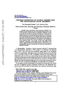
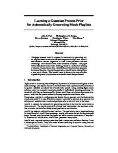
3.2 Nonlinear regression example As an illustrative example, we use a simple one-dimensional nonlinear function: y = sin(10πx sin(x − 0.5)3 ), corrupted with zero mean Gaussian noise, with standard deviation of 0.05. To show how well the system copes with small amounts of data only 30 points are used, which are sampled uniformly in x ∈ [0, 1]. In this range the function has significantly varying derivatives. An interesting aspect of the Gaussian process is its ability to produce good estimates of prediction variance. Figure 1 shows the mean and 2σ contours for y given x. Note how the 2σ contours change over the input-space depending on the proximity of training data.

4 Derivation of Control law The objective of this paper is to control a multi-input, single-output, affine nonlinear system of the form, y(t + 1) = f (x(t)) + g(x(t))u(t) + e(t + 1)

(13)

where x(t) is the state vector at time t, which in this paper will be defined as x(t) = [y(t), . . . , y(t − n), u(t − 1), . . . , u(t−m), v1 (t), . . . , vl (t)], y(t+1) the output, u(t) the current control vector, vi (t), i = 1, . . . , l are external known signals, f and g are smooth nonlinear functions, and g is bounded away from zero. In addition, it is also assumed that the system is minimum phase, as defined in (Chen and Khalil, 1995). For notational simplicity we consider single control input systems, but extending the presentation to vector u(t) is trivial. The noise term e(t) is assumed zero mean Gaussian, but with unknown variance σ 2 .

7

Mean prediction, 2 sigma isoprobability contours and training data 1.2

1

0.8

0.6

0.4

0.2

0

−0.2

−0.4

−0.6

0

0.1

0.2

0.3

0.4

0.5

0.6

0.7

0.8

0.9

1

(a) Model mean and 2σ contours, with target function and training data

Figure 1: Modelling a nonlinear function using a Gaussian Process prior. Model mean and 2σ contours, with target function and training data

8

The cost function proposed is: J

= E{(yd (t + 1) − y(t + 1))2 } + (R(q −1 )u(t))2 .

(14)

where yd (t) is a bounded reference signal, the polynomial R(q −1 ) is defined as: R(q −1 ) = r0 + r1 q −1 + . . . + rnr q −nr

(15)

and its coefficients can be used as tuning parameters. Using the fact that Var{y} = E{y 2 } − µ2y , where µy = E{y}, the cost function can be written as: J

= (yd (t + 1) − E{y(t + 1)})2 + Var{y(t + 1)} + (R(q −1 )u(t))2 .

Note that we have not ‘added’ the model uncertainty term, Var{y(t + 1)}, to the classical quadratic cost function – most conventional work has ‘ignored’ it, or have added extra terms to the cost function,or have pursued other sub-optimal solutions (Wittenmark, 1995; Filatov and Unbehauen, 2000).

4.1 Calculation of optimal u(t) Given the cost function (16), and observations to time t, if we wish to find the optimal u(t), we need the derivative of J, ∂J ∂u(t)

= −2 (yd (t + 1) − µy )

∂µy ∂Var{y(t + 1)} + + 2r0 R(q −1 )u(t). ∂u(t) ∂u(t)

(16)

{y} With most models, estimation of Var{y}, or ∂ Var ∂u(t) would be difficult, but with the Gaussian process prior (as-

suming smooth, differentiable covariance functions – see (O’Hagan, 2001)) the following straightforward analytic solutions can be obtained: ∂µy ∂Σ21 −1 = Σ y1 ∂u(t) ∂u(t) 1 T Var{y} = Σ2 − Σ21 Σ−1 1 Σ21 , ∂Var{y} ∂Σ2 ∂ΣT21 ∂Σ21 −1 T = − (Σ21 Σ−1 + Σ Σ ). 1 ∂u(t) ∂u(t) ∂u(t) ∂u(t) 1 21 The covariance function is composed of the sum of two covariance functions Cx and Cu with separate parameters, C([x u], [x0

u0 ]) = Cx (x, x0 ) + uCu (x, x0 )u0 .

(17)

The covariance matrix Σ21 and Σ2 can be expressed in terms of the independent control variable u(t) as follows: Σ21 = Ω1 + u(t)Ω2 Σ2 = Ω3 + Ω4 u(t)2 , 9

(18) (19)

where Ω1 = Cx (x(t), Φ1 ), Ω2 = Cu (x(t), Φ1 ).∗U1 , where .∗ indicates elementwise multiplication of two matrices. Ω3 = Cx (x(t), x(t)), and Ω4 = Cu (x(t), x(t)). The final expressions for µy and Var{y} are: −1 µy = Ω1 Σ−1 1 y1 + Ω2 Σ1 y1 u(t), T Var{y} = Ω3 + Ω4 u(t)2 − (Ω1 + u(t)Ω2 )Σ−1 1 (Ω1 + u(t)Ω2 ) .

Taking the partial derivatives of the variance and the mean expressions and replacing their values in (16), it follows: ∂J ∂u(t)

¡ ¢ −1 −1 T = −2 yd (t + 1) − Ω1 Σ−1 1 y1 − Ω2 Σ1 y1 u(t) (Ω2 Σ1 y1 ) + 2Ω4 u(t) − −1 T T −1 2Ω1 Σ−1 1 Ω2 − 2u(t)Ω2 Σ1 Ω2 ) + 2r0 R(q )u(t).

At

∂J ∂u(t)

(20)

= 0, the optimal control signal is obtained as: u(t) =

−1 −1 T T −1 + · · · + r q −nr )u(t) (yd (t + 1) − Ω1 Σ−1 nr 1 y1 )(Ω2 Σ1 y1 ) + Ω1 Σ1 Ω2 − r0 (r1 q . −1 T −1 −1 2 T r0 + Ω4 − Ω2 Σ1 Ω2 + Ω2 Σ1 y1 (Ω2 Σ1 y1 )

(21)

Note that equation (21) can also be presented as u(t) =

−1 T −1 + · · · + r q −nr )u(t) (yd (t + 1) − Ω1 Σ−1 nr 1 y1 )(Ω2 Σ1 y1 ) + α(t) − r0 (r1 q . −1 T r02 + β(t) + Ω2 Σ−1 y (Ω Σ y ) 1 2 1 1 1

(22)

−1 T T where α(t) = Ω1 Σ−1 1 Ω2 , and β(t) = Ω4 − Ω2 Σ1 Ω2 . If we had not included the variance term in cost function

(16), or if we were in a region of the state-space where the variance was zero, the optimal control law would be equation (22) with α = β = 0. We can therefore see that analysing the values of α and β is a promising approach to gaining insight into the behaviour of the new form of controller. These terms make a control effort penalty constant, or regulariser unnecessary in many applications. In the experiments in this paper where we include α(t) and β(t), we set r02 = 0. For systems linear in u(t), β(t) does not vary with x(t), y(t) or yd (t), while α(t) varies with x(t).

4.2 Adapting control behaviour with new data After u(t) has been calculated, applied, and the output observed, we add the information x(t), u(t), y(t + 1) to the training set, and the new Σ1 increases in size to N1 +1×N1 +1. We can then choose to optimise the hyperparameters of the covariance function to further refine the model, or keep the covariance function fixed, and just use the extra data points to improve model performance. Obviously, given the expense of inverting Σ1 for large N , this naive approach will only work for relatively small data sets. For a more general solution, we can potentially incorporate elements of Relevance Vector Machines(Tipping, 2001), or use heuristics for selection of data for use in an active training set, as in e.g. (Seeger et al., 2003). 10

5 Simulation results To illustrate the feasibility of the approach we used it to control several target plants based on noisy observed responses. We start off with only two training points, and add subsequent data to the model during operation. The model has had no prior adaptation to the system before the experiment. Model hyperparameters are adapted after each iteration using a conjugate gradient descent optimisation algorithm. A gamma distribution was used for all hyperparameters, with ω set equal to the initial condition for each variable and shape parameter a = 3, indicating vague knowledge about the variable. The noise term σn , was given a tighter distribution, with a = 5. The covariance functions chosen are the same for all the experiments.

5.1 Linear system As an introductory example, if we have a GP to represent a linear model, for a target system of the form: y(t + 1) = w1T x(t) + w2 u(t) + e(t + 1). In this case, the expressions for the mean and the variance are: µy = = b1 xT + b2 u(t) Var{y} = σn + xT C11 x + xT C12 u + uC21 x + uc22 u. (23) Using equation (16), the control signal is : u(t) = ((yd (t + 1) − x(t)T b1 )b2 + x(t)T C12 − r0 (r1 q −1 + · · · + rnr q −nr )u(t)) (b22 + c22 + r02 )−1 .

(24)

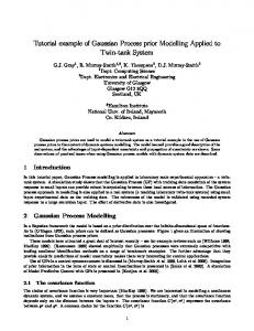
To understand the behaviour of this control law we set R(q −1 ) = r0 and we will create two variables α = x(t)T C12 , and β = c22 . In the experiments in this paper r02 = 0, thus the control signal is: u = ((yd (t + 1) − x(t)T b1 )b2 + α)(b22 + β)−1 . Applying the above control law to the following system: y(t + 1) = 0.5y(t − 1) − 0.3y(t − 2) + 0.2y(t − 3) + 2u(t) − 0.8u(t − 1) + e(t + 1) the algorithm start off with only six training points, and add subsequent data to the model during the operation. The model has no prior adaptation to the system before the experiments. Figure 2 shows the effects of α and β in 11

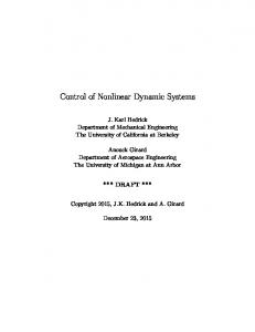
the early stages of the closed loop response. Note the increases in β(t) after the step changes, and the significant decrease once the system covers the space between x = ±1. If the hyperparameters are not updated, then the convergence is much slower, as can be seen in Figure 3.

5.2 Non-linear systems 5.2.1 Nonlinear system 1 Let non-linear system 1 be: y(t + 1) = f (x(t)) + g(x(t))u(t) + e(t + 1) where x = y(t), f (x) = sin(y(t))+cos(3y(t)) and g(x) = 2+cos(y(t)), subject to noise with variance σ 2 = 0.001 (Fabri and Kadirkamanathan, 1998). Note how in Figure 4 β is large in the early stages of learning, but decreasing with the decrease in variance, showing how the regularising effect enforces caution in the face of uncertainty, but reduces caution as the model accuracy increases. In terms of the hyperparameters, most hyperparameters have converged by about 30 data points. The noise parameter σn decreases with increasing levels of training data. After this point the control signal u is also fairly smooth, despite the noisy nature of the data. α can be seen to be larger in higher variance regions, essentially adding an excitatory component which decreases with the decrease in model uncertainty, and in this example plays almost no role after about iteration 30. Figure 5 shows control performance on the same system where the variance part of the cost function is ignored (i.e. α and β are removed from the control law. In order to achieve any reasonable control behaviour, we set r0 = 0.5. As can be seen in the figure, the system still tracks the trajectory, and after iteration 30 there is little visible difference between the two control laws, but ignoring the variance does lead to the use of greater control effort, with larger model uncertainty in the early stages of learning. The hyperparameter estimates also fluctuate much more in the early stages of learning, when variance is not considered, although both systems converge on similar values after the initial stages. The constant nature of r0 as a regularising term, as opposed to the dynamically changing α(t), β(t) makes controller design more difficult, as we can see that in early stages of learning it tends to be too small, reducing robustness, while later it is larger than α(t), β(t) damaging performance. We now plot the nonlinear mappings involved in non-linear system 1, to give the reader a clearer impression of the adaptation of the system. The surfaces in figure 7 show the development in the mean mapping from x(t), u(t) to y(t + 1) as the system acquires data, taken from the simulation shown in figure 4 at t = 3, 20, 99. For comparison,

12

Linear system 2 yd Mu Y −2σ +2σ

yd(k),y(k),ye(k)

1

0

−1

−2

0

10

20

30

40

50 k

60

70

80

90

100

0

10

20

30

40

50 k

60

70

80

90

100

1

u(k)

0.5

0

−0.5

−1

(a) Simulation of linear GP-based controller

Linear system

0

Linear system

1

10

10

ardy(t−1) ardy(t−2) ardy(t−3) ardu(t−1) v0 σn σu

−1

beta(k)

10

0

10 −2

−3

10

0

10

20

30

40

50 k

60

70

80

90

100

parameters

10

−1

10

0.1

alpha(k)

0.05 −2

10 0

−0.05

−0.1

−3

0

10

20

30

40

50 k

60

70

80

90

100

(b) α and β (regularisation term)

10

0

10

20

30

40

50 k

60

70

80

90

100

(c) Covariance function hyperparameters

Figure 2: Simulation results on the identification and control of the linear system, showing modelling accuracy, control signals, tracking behaviour and levels of α and β at each stage.

13

Linear system 3 yd Mu Y −2σ +2σ

yd(k),y(k),ye(k)

2 1 0 −1 −2 −3

0

10

20

30

40

50 k

60

70

80

90

100

0

10

20

30

40

50 k

60

70

80

90

100

1.5 1

u(k)

0.5 0 −0.5 −1 −1.5

(a) Simulation of linear GP-based controller

Linear system

−1.2

beta(k)

10

−1.4

10

−1.6

10

0

10

20

30

40

50 k

60

70

80

90

100

0

10

20

30

40

50 k

60

70

80

90

100

0.03 0.02

alpha(k)

0.01 0 −0.01 −0.02 −0.03

(b) α and β (regularisation term)

Figure 3: Simulation results on the identification and control of the linear system, without updating the hyperparameters, showing modelling accuracy, control signals, tracking behaviour and levels of α and β at each stage. 14

Nonlinear system 1 3 yd Mu Y −2σ +2σ

yd(k),y(k),ye(k)

2 1 0 −1 −2 −3

0

10

20

30

40

50 k

60

70

80

90

100

0

10

20

30

40

50 k

60

70

80

90

100

1.5 1

u(k)

0.5 0 −0.5 −1

(a) Simulation of nonlinear GP-based controller

Nonlinear system 1

1

Nonlinear system 1

1

10

10

ardx v0 σn Cu ardx Cu v0

0

beta(k)

10

−1

10

0

10 −2

−3

10

0

10

20

30

40

50 k

60

70

80

90

100

parameters

10

−1

10

0.2

alpha(k)

0.15 −2

10

0.1 0.05 0 −0.05

−3

0

10

20

30

40

50 k

60

70

80

90

100

(b) α and β (regularisation term)

10

0

10

20

30

40

50 k

60

70

80

90

100

(c) Covariance function hyperparameters

Figure 4: Simulation results for nonlinear system 1, showing modelling accuracy, control signals, tracking behaviour and levels of α and β at each stage.

15

Nonlinear system 1 4 yd Mu Y −2σ +2σ

yd(k),y(k),ye(k)

2 0 −2 −4 −6

0

10

20

30

40

50 k

60

70

80

90

100

0

10

20

30

40

50 k

60

70

80

90

100

1.5 1

u(k)

0.5 0 −0.5 −1 −1.5

(a) Simulation of nonlinear GP-based controller

Nonlinear system 1

1

Nonlinear system 1

1

10

10

ardx v0 σn Cu ardx Cu v0

0

beta(k)

10

−1

10

0

10 −2

−3

10

0

10

20

30

40

50 k

60

70

80

90

100

parameters

10

−1

10

0.3 0.25

alpha(k)

0.2 −2

10

0.15 0.1 0.05 0 −0.05

−3

0

10

20

30

40

50 k

60

70

80

90

100

(b) α and β (regularisation term)

10

0

10

20

30

40

50 k

60

70

80

90

100

(c) Covariance function hyperparameters

Figure 5: Simulation results on nonlinear system 1, without including the α and β terms linked to the model variance in the control law. Data shows modelling accuracy, control signals and tracking behaviour.

16

6 4

y(t+1)

2 0 −2 −4 −6

2 1

2 1

0 0

−1

−1 −2

−2

u(t)

x(t)

Figure 6: True surface (mesh) of nonlinear system 1, y(t + 1) = f (x(t), u(t)) = sin(x(t)) + cos(3x(t)) + (2 + cos(x(t)))u(t), over the space x × u. figure 5.2.1 shows the true mapping. Examining the surfaces in figure 7 we can see how the nonlinear mapping adapts gradually given increasing numbers of data points, but we also see that the standard deviation of the mapping also evolves in an appropriate manner, indicating clearly at each stage of adaptation the model uncertainty over the state-space. In the final plot, Figure 7(f) we can see a uniformly low uncertainty in the areas covered by data, but a rapid increase in uncertainty as we move beyond that in the x-axis. Note that the uncertainty grows much more slowly in the u-axis because of the affine assumption inherent in the covariance function, which constrains the freedom of the model. 5.2.2 Nonlinear system 2 The second nonlinear example considers the following non-linear functions: f (x(t)) = g(x) =

y(t)y(t − 1)y(t − 2)u(t − 1)(y(t − 2) − 1) 1 + y(t − 1)2 + y(t − 2)2 1 1 + y(t − 1)2 + y(t − 2)2 17

2

6 4

1.5

σ(t+1)

y(t+1)

2 0

1

−2 0.5

−4 −6

0

2

2

1

1

2 1

0

2

0

−1

0

−1

−1 −2

1

0 −1 −2

−2

u(t)

−2

u(t)

x(t)

x(t)

(b) σ(x, u)

(a) At 3 datapoints

2

6 4

1.5

σ(t+1)

y(t+1)

2 0

1

−2 0.5

−4 −6

0

2

2

1

1

2 1

0

2

−1

0

−1

−1 −2

1

0

0

−1 −2

−2

u(t)

−2

u(t)

x(t)

x(t)

(d) σ(x, u)

(c) At 20 datapoints

2

6 4

1.5

σ(t+1)

y(t+1)

2 0

1

−2 0.5

−4 −6

0

2

2

1

1

2 1

0

2

−1

−1 −2

−2 x(t)

(e) At 99 datapoints

0

−1

−1 −2

u(t)

1

0

0

−2

u(t)

x(t)

18 (f) σ(x, u)

h , where x =

iT y(t) y(t − 1) y(t − 2) u(t) u(t − 1)

(Narendra and Parthasarathy, 1990). The system

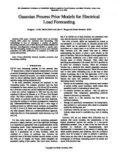
noise has a variance σ 2 = 0.001, and we had 6 initial data points. The results are shown in Figure 8. Again, the trend of decreasing α and β can be seen, although they do increase in magnitude following changes in the system state towards higher uncertainty regions, showing that the control signal will be appropriately damped when the system moves to a less well-modelled area of the state-space. The hyperparameters in Figure 8(c) make few rapid changes, seeming well-behaved during learning.

6 Conclusions This work has presented a novel adaptive controller based on non-parametric models. The control design is based on the expected value of a quadratic cost function, leading to a controller that not only will minimise the squared difference between the reference signal and the expected value of the output, but will also try to minimise the variance of the output, based on analytical estimates of model uncertainty. This leads to a robust control action during adaptation, and when extended to multi-step ahead prediction, forms the basis of full dual control with implicit excitatory components. Simulation results, considering linear and non-linear systems, demonstrate the interesting characteristics of this type of adaptive control algorithm. The GP models are capable of high performance, with or without priors being placed on their hyperparameters. Use of gamma prior distributions led to increased robustness and higher performance in the early stages of adaptation with very few data points, but the relative advantage decreases with the amount of initial data available, as would be expected.

6.1 Outlook GP’s have been successfully adopted from their statistics origins by the neural network community (Williams, 1998). This paper is intended to bring the GP approach to the attention of the control community, and to show that the basic approach is a competitive approach for modelling and control of nonlinear dynamic systems, even when little attempt has been made to analyse the designer’s prior knowledge of the system – there is much more that can be taken from the Bayesian approach to use in the dual control and nonlinear control areas. Further work is underway to address the control of multivariable systems, nonminimum-phase systems and implementation efficiency issues. The robust inference of the GP approach in sparsely populated spaces makes it particularly promising in multivariable and high-order systems.

19

2

yd(k),y(k),ye(k)

1 0 −1 −2 −3

0

20

40

60

80

100

120

140

160

180

100

120

140

160

180

k

3 2

u(k)

1 0 −1 −2

0

20

40

60

80 k

(a) Simulation of nonlinear GP-based controller

15

0.25 0.2 beta(k)

10 0.15

5

0.1 0.05

0

20

40

60

80

100

120

140

160

180

k −3

3

x 10

hyperparameters

0 0

−5

−10

2

alpha(k)

1

−15

0 −1

−20

−2 −3 −4

0

20

40

60

80

100

120

140

160

180

−25

0

20

40

60

80

100

120

140

160

180

k

k

(b) α and β (regularisation term)

(c) Covariance function hyperparameters

Figure 8: Simulation results for nonlinear system 2, showing modelling accuracy, control signals, tracking behaviour and levels of α and β at each stage.

20

7 Acknowledgements Both authors are grateful for support from FONDECYT Project 700397 and the Hamilton Institute. RM-S gratefully acknowledges the support of the Multi-Agent Control Research Training Network supported by EC TMR grant HPRN-CT-1999-00107, and the EPSRC grant Modern statistical approaches to off-equilibrium modelling for nonlinear system control GR/M76379/01.

References Agarwal, M. and D. E. Seborg (1987). Self-tuning controllers for nonlinear systems. Automatica (2), 209–214. Bittanti, S. and L. Piroddi (1997). Neural implementation of GMV control shemes based on affine input/output models. Proc. IEE Control Theory Appl. (6), 521–530. Chen, F.C. and H. Khalil (1995). Adaptive control of a class of nonlinear discrete-time systems. IEEE. Trans. Automatic Control 40(5), 791–801. Fabri, S. and V. Kadirkamanathan (1998). Dual adaptive control of stochastic systems using neural networks. Automatica 14(2), 245–253. Filatov, N.M. and H. Unbehauen (2000). Survey of adaptive dual control methods. Proc. IEE Control Theory Appl. (1), 119–128. Filatov, N.M., H. Unbehauen and U. Keuchel (1997). Dual pole placement controller with direct adaptation. Automatica 33(1), 113–117. Girard, A., C. E. Rasmussen, J. Quinonero-Candela and R. Murray-Smith (2003). Gaussian process priors with uncertain inputs – application to multiple-step ahead time series forecasting. In: Advances in Neural Information processing Systems 15 (S. Becker, S. Thrun and K. Obermayer, Eds.). Leith, D.J., R. Murray-smith and W.E. Leithhead (2000). Nonlinear structure identification: A gaussian process prior/velocity-based approach. In: Proceedings of Control 2000. Cambridge, U.K. Liang, F. and H.A. ElMargahy (1994). Self-tuning neurocontrol of nonlinear systems using localized polynomial networks with CLI cells. In: Proceedings of the American Control Conference. Baltimore, Maryland. pp. 2148–2152. 21

Murray-Smith, R. and A. Girard (2001). Gaussian process priors with ARMA noise models. In: Proceedings of the Irish Sgnals and Systems Conference. Maynooth, Ireland. pp. 147–152. Murray-Smith, R. and D. Sbarbaro (2002). Nonlinear adaptive control using non-paramtric gaussian process prior models. In: Proceedings of the 15th IFAC world congress. Barcelona, Spain. Murray-Smith, R., T.A. Johansen and R. Shorten (1999). On transient dynamics, off-equilibrium behaviour and identification in blended multiple model structures. In: Proceedings of the European Control Conference. Karlsruhe, Germany. pp. BA–14. Narendra, K.S. and P. Parthasarathy (1990). Identification and control of dynamical systems using neural networks. IEEE. Trans. Neural Networks 1(1), 4–27. Neal, R.M. (1997). Monte Carlo implementation of Gaussian process models for Bayesian regression and classification. Technical Report 9702. Department of Statistics, University of Toronto. O’Hagan, A. (1978). On curve fitting and optimal design for regression (with discussion). Journal of the Royal Statistical Society B(40), 1–42. O’Hagan, A. (2001). Some Bayesian numerical analysis. In: Bayesian Statistics 4 (J.M Bernardo, J.O. Berger, A.P. Dawid and F.M. Smith, Eds.). Oxford University Press. pp. 345–363. Rasmussen, C.E. (1996). Evaluation of Gaussian Process and other Methods for non-linear regression. PhD thesis. Department of Computer Science, University of Toronto. Sbarbaro, D., N.M. Filatov and H. Unbehauen (1998). Adaptive dual controller for a class of nonlinear systems. In: Proceedings of the IFAC Workshop on Adaptive systems in Control and Signal Processing. Glasgow, U.K.. pp. 28–33. Seeger, M., C Williams and D.W. Lawrence (2003). Fast forward selection to seep up sparce Gaussian process regression. In: Proceedings of the Ninth International Workshop on AI and Statistics. Shi, J.Q, R. Murray-Smith and D. M. Titterington (2003). Bayesian regression and classification using mixtures of multiple Gaussian processes. International Journal of Adaptive Control and Signal Processing 17(3), –. Solak, E., R. Murray-Smith, W. E. Leithead, D. J. Leith and C. E. Rasmussen (2003). Derivative observations in Gaussian process models of dynamic systems. In: Advances in Neural Information processing Systems 15 (S. Becker, S. Thrun and K. Obermayer, Eds.). 22

Tipping, M. E. (2001). Sparse Bayesian learning and the relevance vector machine. Journal of Machine Learning Research 1, 211–244. Williams, C.K. (1998). Prediction with Gaussian process: From linear regression to linear prediction and beyond. In: Learning and Inference in Graphical Models (M.I. Jordan, Ed.). Kluwer. pp. 599–621. Wittenmark, R. (1995). Adaptive dual control methods: An overview. In: Proceedings of the 5th IFAC Symposium on Adaptive systems in Control and Signal Processing. Budapest. pp. 67–92.

23