system noise and Gaussian measurement noise, respectively. ... The contribution of this paper is the GPIL algorithm for system identification in nonlinear ...
System Identification in Gaussian Process Dynamical Systems
Ryan Turner University of Cambridge
Marc Peter Deisenroth University of Cambridge
Carl Edward Rasmussen University of Cambridge
Inference and learning in linear dynamical systems have long been studied in signal processing, machine learning, and system theory for tracking, localization, and control. In the linear Gaussian case, closed form solutions to inference and learning, also called system identification, are known as the Kalman Filter. For nonlinear dynamical systems (NLDSs), inference and system identification typically require approximations, such as the Extended Kalman Filter (EKF). We consider the case of the NLDS being given by the state-space formulation xt = f (xt−1 ) + �t ∈ RM ,
yt = g(xt ) + ν t ∈ RD ,
(1)
where the latent state x evolves according to a Markovian process. At each time instance t, we obtain a measurement yt which depends on the latent state xt . The terms � and ν denote Gaussian system noise and Gaussian measurement noise, respectively. Assume for a moment that the transition function f : RM → RM and the measurement function g : RM → RD in Eq. (1) are known and a sequence Y = y1 , . . . , yT of measurements has been obtained. Then, inference aims to determine a posterior distribution over the latent state sequence X := x1:T . The requirement for inference in latent space is that the transition function f and the measurement function g are known. The contribution of this paper is the GPIL algorithm for system identification in nonlinear dynamic systems for the special case where f and g are described by Gaussian processes (GPs). We learn GP models for both the transition function f and measurement function g without the necessity of ground truth observations of the latent states. General Setup To train a GP, training inputs and training targets are required. Here, training inputs in latent space are not available since the latent states are not observed. Therefore, to learn the GPs GP f and GP g for f and g, we parameterize them by pseudo training sets, which are similar to the pseudo training sets used in sparse GP approximations [3]. The pseudo training set for GP f consists of N independent pairs of states xi and successor states f (xi )+�i . The parameters of GP f are then given by the kernel hyper-parameters, the pseudo training inputs α = {αi ∈ RM }N i=1 and the pseudo training targets β = {β i ∈ RM }N . GP is parameterized by kernel hyper-parameters, pseudo g i=1 D N training inputs ξ = {ξ i ∈ RM }N in latent space and pseudo training targets υ = {υ ∈ R }i=1 i i=1 in observed space. The role of these pseudo data sets, is simply to provide a flexible parameterization of distributions over nonlinear functions, f and g. Note that the pseudo training sets are not given by a time series x1:T and the corresponding measurements y1:T . Given the GP “parameters”, we predict according to xti = fi (xt−1 ) + �ti ∼ GP f (xt−1 |α, β i ),
ytj = gj (yt ) + νtj ∼ GP g (xt |ξ, υ j ) ,
where xti is the ith dimension of xt and ytj is the j th dimension of yt . System identification determines appropriate “parameters” for GP f and GP g , such that the time series y1:T can be explained. We use the Expectation Maximization (EM) algorithm to determine the “parameters” of both GP models. EM iterates between two steps. In the E-step (inference step), we determine a posterior distribution p(X|Y, Θ) on the hidden states for a fixed parameter setting Θ. In the M-step, we find parameters Θ∗ of the GP state-space model that maximize the expected 1
log-likelihood Q = EX [log p(X, Y|Θ)], where the expectation is taken with respect to p(X|Y, Θ), the E-step distribution. System Identification with EM For analytic inference (E-step), we extend the filtering algorithm of [1] to smoothing in GP statespace models. The algorithm is based on approximate moment matching but we do not give the details here. In the M-Step, we seek the parameters Θ that maximize the likelihood lower bound Q = EX [log p(X, Y|Θ)] where the expectation is computed under the distribution from the E-Step, meaning X is treated as the random variable. We decompose Q into T T X X Q = EX [log p(X, Y|Θ)] = EX log p(x1 |Θ) + log p(xt |xt−1 , Θ)+ log p(yt |xt , Θ) . (2) | {z } t=1 | {z } t=2 Transition
Measurement
In the following we use the notation µi (x) = Efi [fi (x)] to refer to the expected value of the ith dimension of f when evaluated at x. Likewise, σi2 (x) = Varfi [fi (x)] refers to the variance of the output of ith dimension of f when evaluated at x. We focus on finding a lower bound approximation to the contribution from the transition function, � � � � M 1X (xti − µi (xt−1 ))2 2 + const. (3) EX + E EX [log p(xt |xt−1 , Θ)] = − log σ (x ) X t−1 i 2 i=1 σi2 (xt−1 ) {z } | | {z } Data Fit Term
Complexity Term
Eq. (3) amounts to an expectation over a nonlinear function of a normally distributed random variable since X is approximately Gaussian (E-step). Note that in contrast to most other NLDS system identification algorithms the variance of f (xt−1 ) depends on the location of xt−1 . Data fit. We first consider the data fit term in eq. (3), which is an expectation over the square Mahalanobis distance. For tractability, we approximate the expectation of the ratio � � � � EX (xti − µi (xt−1 ))2 (xti − µi (xt−1 ))2 EX ≈ . (4) σi2 (xt−1 ) EX [σi2 (xt−1 )] Complexity penalty. We next approximate the complexity penalty in eq. (3), which penalizes uncertainty. The contribution from the logarithm can be lower bounded by Jensen’s inequality, � � � � EX log σi2 (xt−1 ) ≤ log EX σi2 (xt−1 ) . (5) Nearly identical expressions to and eq. (4) and eq. (5) exist for the measurement model. Results We evaluate our EM based system identification on both real and synthetic data sets using onestep-ahead prediction. We compare GPIL predictions to eight other methods, the time independent model (TIM) with yt ∼ N (µc , Σc ), the Kalman filter, the UKF, the EKF, NDFA, GPDM, the Autoregressive GP (ARGP) trained on a set of pairs (yi , yi+1 ), and the GP-UKF [2], which uses the GPIL pseudo training set. Note that the EKF, the UKF, and the GP-UKF require access to the true functions f and g. For synthetic data, f and g are known, for the real data set, we used “true” functions that resemble the mean functions of the GPIL learned GP models. Real data. We use historical snowfall data in Whistler, BC, Canada to evaluate GPIL on real data. We evaluate the models’ ability to predict next day’s snowfall using 35 years of test data; we trained on daily snowfall from Jan. 1 1972–Dec. 31 1973 and tested on next day predictions for 1974–2008. The results are shown in table 1. Snowfall time series have many observations of zero, corresponding to days when it does not snow. The GPIL learns a GP model for a close-to-linear stochastic latent transition function (Fig. 1(a)). A possible interpretation of the results is that the daily precipitation is almost linear. Note that for positive temperatures no snow occurs, which results in a hinge measurement model. The GPIL learns a hinge like function for the measurement model, Fig. 1(b), which allows for predicting a high probability of zero snowfall the next day. The Kalman filter is incapable of such predictions since it assumes linear functions f and g, respectively. 2
5 4
4
4
3
3
posterior mean
snowfall in log−cm
pseudo targets
3
f(x)
2 2
1 1
0 −1
0
2
1
0
posterior mean
−2 −3
pseudo targets
−2
−1
0
1
2
3
−1
4
5
6
−1 1
x
(a) Learned GP model for the stochastic transition function (real data set).
0.1
0.01
−1
0
1
2 x
3
4
5
(b) Learned measurement function with log histogram (real data set)
Figure 1: The gray area is twice the predictive standard deviation. The histograms (black) represents the marginal distribution on xt (left panel) and on yt (right panel).
Table 1: Comparison of the GPIL with eight other methods on the sinusoidal dynamics example and the Whistler snowfall data. We trained on daily snowfall from Jan. 1 1972–Dec. 31 1973 and tested on next day predictions for 1974–2008. We report the NLL per data point and the RMSE as well as the NLL 95% error bars. We do not report results for GPDM on the real data since it was too slow to run on the large test set.
general
requires prior knowledge
Method TIM Kalman ARGP NDFA GPDM GPIL ? UKF EKF GP-UKF
NLL synth. 2.21±0.0091 2.07±0.0103 1.01±0.0170 2.20±0.00515 3330±386 0.917 ± 0.0185 4.55±0.133 1.23±0.0306 6.15±0.649
RMSE synth. 2.18 1.91 0.663 2.18 2.13 0.654 2.19 0.665 2.06
NLL real 1.47±0.0257 1.29±0.0273 1.25±0.0298 14.6±0.374 N/A 0.684 ± 0.0357 1.84±0.0623 1.46±0.0542 3.03±0.357
RMSE real 1.01 0.783 0.793 1.06 N/A 0.769 0.938 0.905 0.884
Discussion and Conclusions We proposed a general method for inference and learning (system identification) in nonlinear stochastic state-space models, where both the transition function and the measurement function are modeled by GPs. The GPs are parameterized by their hyper-parameters and a pseudo training set that are similar to the pseudo training sets in sparse GP approximations. Based on EM, where the inference step can be performed in closed form, we learn the parameters of the transition GP and the measurement GP, respectively. Note that in our model, the latent states xt are never observed directly. We solely have access to noisy measurements yt to train the latent dynamics and measurement functions. By contrast, [1] and [2] require direct access to ground truth observations of a latent state sequence to train the dynamics model. We showed that our learning approach can successfully learn nonlinear (latent) dynamics based on noisy observations only. Moreover, in our experiments, our algorithm performs better than commonly used approaches for time series predictions.
References [1] M. P. Deisenroth, M. F. Huber, and U. D. Hanebeck. Analytic Moment-based Gaussian Process Filtering. In L. Bouttou and M. L. Littman, editors, Proceedings of the 26th International Conference on Machine Learning, pages 225–232, Montreal, Canada, June 2009. Omnipress. [2] J. Ko and D. Fox. GP-BayesFilters: Bayesian Filtering using Gaussian Process Prediction and Observation Models. Autonomous Robots, 27(1):75–90, July 2009. [3] E. Snelson and Z. Ghahramani. Sparse Gaussian processes using pseudo-inputs. In Advances in Neural Information Processing Systems 18, pages 1257–1264. The MIT Press, 2006.
3