Self-Tuning Routing Algorithms Howard Tripp
Robert Hancock
Abstract—Self adapting protocols are attractive theoretically because they converge towards optimal operation, and practically because they eliminate classes of misconfiguration error. In order to achieve self adaption, a protocol needs to gather state information upon which to base decisions. This paper begins to address these issues by investigating the trade-off surrounding the rate at which information needs to be gathered. If information is gathered too frequently, the overhead outweighs the benefit; but gathering too infrequently means that the state information is inaccurate and sub-optimal. This trade-off is investigated analytically on some simplified abstract problems. The results reveal how there are large and distinct regions where the routing strategy is degenerate (i.e. maximal or minimal state gathering). Moreover there are sharp transitions between these regions, providing useful insight to the next stage of the research. This will look at more realistic network models, a wider class of routing algorithms, and reduced assumptions about wireless characteristics.
I. I NTRODUCTION
T
HERE are many benefits provided by self-adapting or “intelligent” protocols. They can respond automatically to network changes; they allow different parts of the network to have different locally optimal configurations; and the complexity requirements for practical implementation are reduced. In particular, self-adaptation is a form of robustness, but rather than robustness to particular events, we are looking at robustness to variability in network operating conditions or protocol misconfiguration. A self-adapting protocol is essentially a feedback (or feedforward) control loop whereby protocol parameters are adjusted based on detected network status, in order to drive the system towards optimal operation. This control loop needs an understanding of how to achieve optimal performance for a given network state, and a mechanism to obtain network state, both of which are nontrivial. Optimal performance could be defined in terms of latency and throughput of individual or aggregated flows, power or radio resource efficiency, reliability of connectivity, and so on. Indeed, the optimisation goal could be different for different participants, in the same way as endhost utilities in the NUM formulation for transport protocols. Howard Tripp and Robert Hancock are with Roke Manor Research Ltd, Email: howard.tripp;
[email protected]. Jim Kurose is with University of Massachusetts This research was sponsored by the U.S. Army Research Laboratory and the U.K. Ministry of Defence and was accomplished under Agreement Number W911NF-06-3-0001. The views and conclusions contained in this document are those of the author(s) and should not be interpreted as representing the official policies, either expressed or implied, of the U.S. Army Research Laboratory, the U.S. Government, the U.K. Ministry of Defence or the U.K. Government. The U.S. and U.K. Governments are authorized to reproduce and distribute reprints for Government purposes notwithstanding any copyright notation hereon.
Jim Kurose
Fig. 1.
Diamond network model
The mechanisms for gathering state also has difficulties such as what information is actually useful? Is the information available locally or in remote parts of the network? What accuracy of information is required? In general, obtaining state information does not come for free, and that there must be some associated overhead to obtain and distribute it. A fundamental question is therefore what is the trade-off between state gathering overhead and protocol performance? This paper addresses this trade-off challenge for a particular, simplified network model, in order to understand how routing algorithm parametrisation and control of signalling overhead can be formulated as an optimisation problem. The results indicate that there are many network conditions where is there is no benefit to gathering state and only small changes in these conditions tip the balance to when state is extremely useful. II. P ROBLEM FORMULATION A. Simplified representation In order to analyse the state overhead trade-off a highly simplified representation is chosen see Fig 1. In this model a source, S, wishes to transmit data to a destination, D. There are two different paths that this transmission can take, via relay nodes R1 or R2 . There are completely reliable links between S and each of the R’s, however the links from the R’s to D, are up and down based on a two state Markov model. These links have identical properties but are independent, and each time step remain up with a probability p, or remain down with a probability q, in line with previous work [1]. This scenario is an abstraction with constraints to restrict the most obvious solution of broadcasting to both relays simultaneously. This constraint is introduced to simulate network properties that reveal themselves at larger scales, without having to model the large-scale networks themselves. The critical abstraction is that there is a choice to be made between using the upper or lower path for data transmission, and that the source gathers status information to help optimise this choice. In the real world there are two possible reasons why such a choice might be necessary:
• •
S can’t broadcast efficiently to R1 and R2 . It is for some reason much less efficient for one of R1 or R2 to forward the data than the other.
There are many generalisations of this model that are being considered in ongoing work including larger numbers of relay nodes, different and/or variable link-state models, multiple source destinations and transmission penalty functions. B. Transmission strategy The transmission strategy considered here is a time slot model where the source has a choice of three different actions that can be performed in any given time slot: • •
Request (and receive) the current state from both relays (simultaneously) Transmit data via R1 OR via R2
The strategy used by the source is a cyclic two phase operation. The first part is called the “probing phase”, in which the source continually requests status. When one or more of the relays is seen to be in the up state, the “sending phase” begins. In the sending phase the source sends data over the relay that is up (arbitrary choice if both are up) for a fixed number of timeslots, TS . In the TS + 1 timeslot the source returns to the probing phase. The length of the probing phase is dependent on what underlying link-state transitions occur. The length of the sending phase is controlled by the parameter TS , the choice of which defines the strategy. A low TS implies that status is being frequently requested (potentially wasting time slots available for data transmission), where as a high TS increases the chance of data being sent via the wrong relay for an extended period, and hence risks not making proper use of the alternative paths. Choosing a high TS not only potentially reduces the source’s goodput (by forwarding to node that cannot forward the data onwards), but may also waste the resources of the relay (e.g. unnecessary battery depletion) or resources of other traffic flows (e.g. reducing overall network capacity). This wider network effect can be modeled by introducing a penalty function to penalise sources for unnecessarily transmitting data to a relay. Our optimisation goal is to maximise the long term average goodput (data delivered to D), and we do this by varying TS which directly controls the amount of overhead incurred. III. I NITIAL R ESULTS This model can be solved analytically and the details of the mathematics (along with additional results) are given in a complimentary report [2]. In outline, we model the sequence of probing/sending cycles as a Markov chain. For each cycle, the total goodput is the expected throughput during the sending phase, and the time interval is TS plus the length of the probing phase TP . The latter depends in principal on the entire history of the network, because the state at the end of the sending phase, for finite TS , depends on the state at the start. Each cycle is considered as a step in a Markov chain, i.e. a sequence
Fig. 2.
T ∗ as a function of p and q
of TS + TP timesteps, and assuming a stationary distribution1 of that chain, which we call π. As is well known, the stationary distribution is the normalised left eigenvector of the transition matrix for this Markov chain. The critical value is probability of beginning the probing phase in the link down state (since this can be used to calculate the expected value of TP ) which is given by r πdd
1−p−q (1 − r2 )(1 − p)2 = (2 − p − q)2 + 2 1−p 1+q r(2 − p − q)
=
As an example of the results that can be obtained, Fig 2 shows the optimal TS value, called T ∗ , needed to obtain the maximal average goodput over a long sequence of cycles (with no penalty weighting), as a function of the link-stake probabilities p and q. The interpretation of the graph is that there are large regions where the strategy is degenerate (infinite T ∗ ), although the results reveal that this is dependent on the penalty function applied. Another interesting fact is that the boundary between these degenerate and interesting regions is rather sharp: the optimal value for T ∗ rapidly increases to infinity, and there are only small regions of (p, q) space where T ∗ is large but finite. IV. O NGOING WORK The results hint at directions for further investigations. Having determined a formula for the optimal strategy, the source needs to calculate the underlying link-stake probabilities in order to apply it. The probing phase therefore needs to build up a history of state. How much overhead is needed to obtain this history is not yet clear, but the results above can be used to guide the learning strategy. We also intend to investigate more sophisticated network models, both of more complex topologies and more realistic wireless link behaviour. R EFERENCES [1] V. Manfredi, R. Hancock and J. Kurose. Robust Routing in Dynamic Networks. In Annual Conference of the International Technology Alliance, 2008. [2] R. Hancock and H Tripp. Mathematics and analytical results of state overhead in the diamond network. https://www.usukitacs.com/ 1 i.e. a chosen probability distribution of states, with probabilities chosen so that applying the transition matrix returns the same probability distribution.