High-throughput Architecture and Routing Algorithms ...

High-throughput Architecture and Routing Algorithms Towards the Design of Reliable Mesh-based Many-Core Network-on-Chip Systems

Akram Ben Ahmed

A DISSERTATION SUBMITTED IN PARTIAL FULFILLMENT OF THE REQUIREMENTS FOR THE DEGREE OF DOCTOR OF PHILOSOPHY IN COMPUTER SCIENCE AND ENGINEERING

The University of Aizu Graduate Department of Computer and Information Systems Adaptive Systems Laboratory 2015

ii The thesis titled

High-throughput Architecture and Routing Algorithms Towards the Design of Reliable Mesh-based Many-Core Network-on-Chip Systems by

Akram Ben Ahmed is reviewed and approved by:

Chief referee Professor Abderazek Ben Abdallah Professor Toshiaki Miyazaki Professor Tsuneo Tsukahara Professor Junji Kitamichi Senior Associate Professor Hiroshi Saito

The University of Aizu 2015

iii

Dedicated to my lovely Mother, my Father, and to the rest of my Family

iv

High-throughput Architecture and Routing Algorithms Towards the Design of Reliable Mesh-based Many-Core Network-on-Chip Systems Akram Ben Ahmed Submitted for the degree of Doctor of Philosophy March 2015

Abstract Global interconnects are becoming the principal performance bottleneck for high performance Systems-on-Chips (SoCs). Since the main purpose for these systems is to shrink the size of the chip as smaller as possible while seeking at the same time for more scalability, higher bandwidth, and lower latency. Conventional bus-basedsystems are no longer reliable architecture for SoCs due to the lack of scalability and parallelism integration, high latency and power dissipation, and low throughput. During this last decade, Network-on-Chip (NoC) interconnect has been proposed as a promising solution for future SoC designs. It offers more scalability than the sharedbus based interconnection and allows more processors to operate concurrently. Despite the higher scalability and parallelism integration offered by NoC over traditional shared-bus based systems, it is still not an ideal solution for future large scale SoCs. This is due to some limitations such as high power consumption, high cost communication, and low throughput. Recently, merging NoC to the third dimension (3D-NoCs) has been proposed to deal with those problems, as it was a solution offering lower power consumption and higher speed. As 3D-NoC architectures started to show their outperformance and energy efficiency against 2D-NoC systems, questions about their reliability to sustain their performance growth begun to arise. This is mainly due to challenges inherited from both 3D-ICs and NoCs: On one side, the complex nature of 3D-IC fabrics and the

v continuing shrinkage of semiconductor components. Furthermore, the significant heterogeneity in 3D chips which are likely to mix logic layers with memory layers and even more complex technologies increases the fault’s probability in a system. On the other side, the single-point-failure nature of NoC introduces a big concern to their reliability as they are the sole communication medium. As a result, 3DNoC systems are becoming susceptible to a variety of faults caused by crosstalk, electromagnetic interferences, impact of radiations, oxide breakdown, and so on. A simple failure in a single transistor caused by one of these factors may compromise the entire system reliability where the failure can be illustrated in corrupted message delivery, time requirements unsatisfactory, or even sometimes the entire system collapse. In this thesis, we propose 3D-Fault-Tolerant-OASIS (3D-FTO), a robust faulttolerant 3D-NoC router architecture endorsed with reliable and graceful routing algorithms. The proposed design handles a large number of faults in the inputbuffer, crossbar, and links (which are the most susceptible components to faults in 3D-NoC systems) leveraging the inherent structural redundancy in the architecture to work around errors. Contrary to previous works, the proposed system tolerates multiple faults in a single crossbar with no considerable performance degradation. In addition, the used algorithms are always minimal (as long as there exist one minimal path) and with the aid of Random-Access-Buffer (RAB) mechanism, deadlock-freedom is ensured with no significant area nor power overhead. The proposed 3D-FTO system was synthesized using Synopsys Design Compiler at 45nm technology CMOS process technology and its layout is obtained using Cadence SoC Encounter. The evaluation results showed the ability of 3D-FTO to work around different kinds of faults ensuring graceful performance degradation while minimizing the additional hardware complexity and remaining power-efficient.

Declaration The work in this thesis is based on research carried out at the Adaptive Systems Laboratory at the University of Aizu, Japan. No part of this thesis has been submitted elsewhere for any other degree or qualification and it is all my own work unless referenced to the contrary in the text.

c 2015 by Akram Ben Ahmed. Copyright “The copyright of this thesis rests with the author. No quotations from it should be published without the author’s prior written consent and information derived from it should be acknowledged”.

viii

Acknowledgements First of all, I would like to express my thanks and gratitude to my supervisor Prof. Abderazek Ben Abdallah for his support, encouragement and his efforts and guidance to achieve this project. During the past few years spent working under his supervision, he has never stopped believing in my capabilities and he has always pushed me to be a better researcher and person. These words will never be enough to describe my deepest gratitude for him. Second, I would like to thank Prof. Toshiaki Miyazai, Prof. Tsuneo Tsukahara, Prof. Junji Kitamichi, and Prof. Hiroshi Saito of the University of Aizu for taking the time to revise my thesis. Moreover, my sincere gratitude to Prof. Kenichi Kuroda and Prof. Yuichi Okuyama for their help and support during the past three years. Third, I want to thank my beloved parents and the rest of family. Their supportive words and encouraging messages kept me motivated to work harder baring the long distance separating us. I hope that one day I can pay back some of the sacrifices that they have been through so I can be the person that I am now. Last but not least, I would like to thank all my friends back home and in Japan. Especially, the members of the Adaptive Systems Laboratory at the University of Aizu who welcomed me and considered me as one of them. They facilitated my integration in the Japanese society with their valuable adivce making my campus and social life much easier and more comfortable.

ix

Contents 1 Introduction 1.1

1

Background . . . . . . . . . . . . . . . . . . . . . . . . . . . . . . . .

1

1.1.1

System-on-Chips . . . . . . . . . . . . . . . . . . . . . . . . .

1

1.1.2

Network-on-Chips . . . . . . . . . . . . . . . . . . . . . . . . .

3

1.1.3

3D-Network-on-Chips . . . . . . . . . . . . . . . . . . . . . . .

6

1.2

Problems and Motivation . . . . . . . . . . . . . . . . . . . . . . . . .

6

1.3

Thesis objectives and contributions . . . . . . . . . . . . . . . . . . .

7

1.4

Thesis outline . . . . . . . . . . . . . . . . . . . . . . . . . . . . . . .

9

2 On-Chip Interconnects and Reliability 2.1

2.2

2.3

11

Overview of on-Chip interconnect . . . . . . . . . . . . . . . . . . . . 11 2.1.1

Topology . . . . . . . . . . . . . . . . . . . . . . . . . . . . . . 12

2.1.2

Forwarding methods . . . . . . . . . . . . . . . . . . . . . . . 14

2.1.3

Flow control . . . . . . . . . . . . . . . . . . . . . . . . . . . . 18

2.1.4

Routing algorithms . . . . . . . . . . . . . . . . . . . . . . . . 21

2.1.5

Deadlock and Livelock . . . . . . . . . . . . . . . . . . . . . . 23

3D-Network-on-Chip . . . . . . . . . . . . . . . . . . . . . . . . . . . 27 2.2.1

Topology and router architecture . . . . . . . . . . . . . . . . 27

2.2.2

Routing algorithms . . . . . . . . . . . . . . . . . . . . . . . . 30

2.2.3

Through Silicon Via (TSV) . . . . . . . . . . . . . . . . . . . 30

2.2.4

3D-NoC advantages and challenges . . . . . . . . . . . . . . . 32

Reliability in on-chip interconnect . . . . . . . . . . . . . . . . . . . . 34 2.3.1

Reliability and time . . . . . . . . . . . . . . . . . . . . . . . . 34

2.3.2

Failure and main factors . . . . . . . . . . . . . . . . . . . . . 34 x

Contents 2.3.3 2.4

xi Reliability and locality . . . . . . . . . . . . . . . . . . . . . . 36

Conclusion . . . . . . . . . . . . . . . . . . . . . . . . . . . . . . . . . 36

3 Related Work to Fault-Tolerant Techniques in NoCs

37

3.1

Fault-tolerant solutions for 2D-NoC systems . . . . . . . . . . . . . . 37

3.2

Fault-tolerant solutions for 3D-NoC systems . . . . . . . . . . . . . . 38

3.3

3.2.1

Fault-tolerant routing algorithms . . . . . . . . . . . . . . . . 38

3.2.2

Router architecture solutions

. . . . . . . . . . . . . . . . . . 41

Conclusion . . . . . . . . . . . . . . . . . . . . . . . . . . . . . . . . . 43

4 Efficient Fault-tolerant Routing Algorithms for Robust Architectures

45

4.1

Look-Ahead-XYZ Routing Algorithm Overview . . . . . . . . . . . . 45

4.2

Look-Ahead-Fault-Tolerant routing algorithm . . . . . . . . . . . . . 47

4.3

4.2.1

Assumptions . . . . . . . . . . . . . . . . . . . . . . . . . . . . 47

4.2.2

Fault detection . . . . . . . . . . . . . . . . . . . . . . . . . . 48

4.2.3

Algorithm . . . . . . . . . . . . . . . . . . . . . . . . . . . . . 48

4.2.4

Example . . . . . . . . . . . . . . . . . . . . . . . . . . . . . . 51

4.2.5

Weakpoints . . . . . . . . . . . . . . . . . . . . . . . . . . . . 53

Hybrid-Look-Ahead-Fault-Tolerant routing algorithm . . . . . . . . . 55 4.3.1

Algorithm . . . . . . . . . . . . . . . . . . . . . . . . . . . . . 55

4.3.2

Example . . . . . . . . . . . . . . . . . . . . . . . . . . . . . . 56

4.4

Adaptivity . . . . . . . . . . . . . . . . . . . . . . . . . . . . . . . . . 57

4.5

Conclusion . . . . . . . . . . . . . . . . . . . . . . . . . . . . . . . . . 58

5 Reliable Router Architecture and Design for Fault-Tolerant 3DNoC Systems 5.1

60

3D-OASIS-NoC baseline router architecture overview . . . . . . . . . 60 5.1.1

Switching method . . . . . . . . . . . . . . . . . . . . . . . . . 61

5.1.2

Router architecture . . . . . . . . . . . . . . . . . . . . . . . . 61

5.1.3

Input-port circuit . . . . . . . . . . . . . . . . . . . . . . . . . 61

5.1.4

Switch-Allocator circuit . . . . . . . . . . . . . . . . . . . . . 65

Contents 5.2

5.3

xii

Proposed 3D-Fault-Tolerant-OASIS-NoC router architecture . . . . . 67 5.2.1

Random-Access-Buffer mechanism . . . . . . . . . . . . . . . . 69

5.2.2

Traffic-Prediction Unit . . . . . . . . . . . . . . . . . . . . . . 77

5.2.3

Bypass-Link-on-Demand . . . . . . . . . . . . . . . . . . . . . 80

5.2.4

Fault-Control . . . . . . . . . . . . . . . . . . . . . . . . . . . 83

Conclusion . . . . . . . . . . . . . . . . . . . . . . . . . . . . . . . . . 84

6 Evaluation

85

6.1

Evaluation methodology . . . . . . . . . . . . . . . . . . . . . . . . . 85

6.2

Performance evaluation results . . . . . . . . . . . . . . . . . . . . . . 91 6.2.1

Look-Ahead-Fault-Tolerant routing algorithm evaluation . . . 91

6.2.2

Hybrid-Look-Ahead-Fault-Tolerant routing algorithm evaluation . . . . . . . . . . . . . . . . . . . . . . . . . . . . . . . . 95

6.2.3

Random-Access-Buffer and Traffic-Prediction-Unit techniques evaluation . . . . . . . . . . . . . . . . . . . . . . . . . . . . . 103

6.2.4

Bypass-Link-on-Demand technique evaluation . . . . . . . . . 104

6.2.5

3D-Fault-Tolerant-OASIS router evaluation . . . . . . . . . . . 107

6.3

Prototyping results . . . . . . . . . . . . . . . . . . . . . . . . . . . . 115

6.4

Reliability evaluation . . . . . . . . . . . . . . . . . . . . . . . . . . . 120

6.5

Conclusion . . . . . . . . . . . . . . . . . . . . . . . . . . . . . . . . . 121

7 Conclusions

122

7.1

Summary . . . . . . . . . . . . . . . . . . . . . . . . . . . . . . . . . 122

7.2

Future work . . . . . . . . . . . . . . . . . . . . . . . . . . . . . . . . 123

Bibliography

124

A LAFT and HLAFT Routing algorithms implementation in VerilogHDL

145

A.1 LAFT Routing Algorithm (LAFT.v) . . . . . . . . . . . . . . . . . . 149 A.2 HLAFT Routing Algorithm (flag.v) . . . . . . . . . . . . . . . . . . . 156

List of Figures 1.1

SOC Design Complexity Trends [7] . . . . . . . . . . . . . . . . . . .

2

1.2

Conventional SoC architectures: (a) Shared-bus, (b) Point-2-Point . .

3

1.3

Network-on-Chip architecture . . . . . . . . . . . . . . . . . . . . . .

4

2.1

NoC topologies. . . . . . . . . . . . . . . . . . . . . . . . . . . . . . . 13

2.2

Store-and-Forward switching. . . . . . . . . . . . . . . . . . . . . . . 15

2.3

Wormhole switching. . . . . . . . . . . . . . . . . . . . . . . . . . . . 16

2.4

Virtual-Cut-Through switching. . . . . . . . . . . . . . . . . . . . . . 17

2.5

ON/OFF flow control. . . . . . . . . . . . . . . . . . . . . . . . . . . 18

2.6

Credit-based flow control. . . . . . . . . . . . . . . . . . . . . . . . . 19

2.7

ACK/NACK flow control. . . . . . . . . . . . . . . . . . . . . . . . . 20

2.8

Categorization of routing algorithms according to the number of destinations: (a) unicast, (b) multicast. . . . . . . . . . . . . . . . . . . . 21

2.9

Categorization of routing algorithms according to decision locality: (a) distributed, (b) source. . . . . . . . . . . . . . . . . . . . . . . . . 22

2.10 Categorization of routing algorithms according to adaptivity: (a) deterministic, (b) adaptive. . . . . . . . . . . . . . . . . . . . . . . . . . 23 2.11 Categorization of routing algorithms according to minimality: (a) minimal, (b) non-minimal. . . . . . . . . . . . . . . . . . . . . . . . . 24 2.12 Deadlock example in adaptive NoC systems. . . . . . . . . . . . . . . 25 2.13 Virtual-Channel-based router architecture. . . . . . . . . . . . . . . . 25 2.14 Virtual-Output-Queue-based router architecture. . . . . . . . . . . . . 26 2.15 4x4x4 3D-NoC mesh topology. . . . . . . . . . . . . . . . . . . . . . . 28 2.16 3x3x3 3D-NoC Bus Hybrid topology [74]. . . . . . . . . . . . . . . . . 29 xiii

List of Figures

xiv

2.17 TSV channel in a 3D Wafer Level Packaging [87]. . . . . . . . . . . . 31 2.18 3x3 TSV array. . . . . . . . . . . . . . . . . . . . . . . . . . . . . . . 32 4.1

Conventional XYZ routing router pipeline stages. . . . . . . . . . . . 46

4.2

Look-Ahead-XYZ routing router pipeline stages. . . . . . . . . . . . . 47

4.3

Fault information exchange. . . . . . . . . . . . . . . . . . . . . . . . 49

4.4

Look Ahead Fault Tolerant routing algorithm example. . . . . . . . . 52

4.5

Example of fault-tolerant routing: (a) Look-ahead routing (LAFT) (b) Hybrid routing (HLAFT). . . . . . . . . . . . . . . . . . . . . . . 54

4.6

Hybrid-Look-Ahead-Fault-Tolerant routing router pipeline stages. . . 57

5.1

Baseline 3D-OASIS-NoC system architecture. . . . . . . . . . . . . . 62

5.2

Input-port module architecture. . . . . . . . . . . . . . . . . . . . . . 63

5.3

3D-OASIS-NoC flit format. . . . . . . . . . . . . . . . . . . . . . . . . 64

5.4

Switch allocator block diagram. . . . . . . . . . . . . . . . . . . . . . 64

5.5

3D-OASIS-NoC flow control mechanism. . . . . . . . . . . . . . . . . 66

5.6

3D-OASIS-NoC router architecture. . . . . . . . . . . . . . . . . . . . 68

5.7

Example of deadlock-recovery with Random-Access-Buffer. . . . . . . 70

5.8

Random-Access-Buffer for deadlock recovery block diagram. . . . . . 72

5.9

Random-Access-Buffer for deadlock recovery and fault-tolerance block diagram. . . . . . . . . . . . . . . . . . . . . . . . . . . . . . . . . . . 75

5.10 Example of Random-Access-Buffer mechanism for deadlock-recovery and fault-tolerance. Red crosses represent permanent faults, and the green one represents intermittent or transient faults . . . . . . . . . . 76 5.11 Simplified example explaining the use of the Traffic-Prediction-Unit (TPU). . . . . . . . . . . . . . . . . . . . . . . . . . . . . . . . . . . . 78 5.12 Example of Bypass-Link-on-demand. . . . . . . . . . . . . . . . . . . 82 6.1

Matrix multiplication example: The multiplication of an i xk matrix A by a k xj matrix B results in an i xj matrix R. . . . . . . . . . . . . 86

6.2

Simple example demonstrating the Matrix-multiplication calculation.

86

6.3

Task graph of the JPEG encoder . . . . . . . . . . . . . . . . . . . . 87

6.4

Extended task graph of the JPEG encoder . . . . . . . . . . . . . . . 88

List of Figures 6.5

xv

Look-Ahead-Fault-Tolerant routing algorithm latency per flit evaluation with: (a) Transpose (b) Uniform (c) 6x6 Matrix. . . . . . . . . 93

6.6

Look-Ahead-Fault-Tolerant routing algorithm throughput evaluation with: (a) Transpose (b) Uniform (c) 6x6 Matrix. . . . . . . . . . . . . 96

6.7

Hybrid-Look-Ahead-Fault-Tolerant routing algorithm latency per flit comparison results between XYZ, LA-XYZ, LAFT, and HLAFT based 3D-NoC systems with: (a) Transpose; (b) Uniform. . . . . . . . . . . 98

6.8

Hybrid-Look-Ahead-Fault-Tolerant routing algorithm latency per flit comparison results between XYZ, LA-XYZ, LAFT, and HLAFT based 3D-NoC systems with: (a) 6 × 6 Matrix; (b) JPEG. . . . . . . . . . . 99

6.9

Hybrid-Look-Ahead-Fault-Tolerant routing algorithm throughput comparison results between XYZ, LA-XYZ, LAFT, and HLAFT based 3D-NoC systems with: (a) Transpose; (b) Uniform. . . . . . . . . . . 100

6.10 Hybrid-Look-Ahead-Fault-Tolerant routing algorithm throughput comparison results between XYZ, LA-XYZ, LAFT, and HLAFT based 3D-NoC systems with: (a) 6 × 6 Matrix; (b) JPEG. . . . . . . . . . . 101 6.11 Random-Access-Buffer and Traffic-Prediction-Unit latency/flit evaluation with: (a) Transpose; (b) Uniform. . . . . . . . . . . . . . . . . 105 6.12 Random-Access-Buffer and Traffic-Prediction-Unit latency/flit evaluation with: (a) 6 × 6 Matrix; (b) JPEG. . . . . . . . . . . . . . . . 106 6.13 Bypass-Link-on-Demand technique latency/flit evaluation with: (a) Transpose; (b) Uniform. . . . . . . . . . . . . . . . . . . . . . . . . . 108 6.14 Bypass-Link-on-Demand technique latency/flit evaluation with: (a) 6 × 6 Matrix; (b) JPEG. . . . . . . . . . . . . . . . . . . . . . . . . . 109 6.15 3D-Fault-Tolerant-OASIS latency/flit evaluation with: (a) Transpose; (b) Uniform. . . . . . . . . . . . . . . . . . . . . . . . . . . . . . . . . 111 6.16 3D-Fault-Tolerant-OASIS latency/flit evaluation with: (a) 6 × 6 Matrix; (b) JPEG. . . . . . . . . . . . . . . . . . . . . . . . . . . . . . . 112 6.17 3D-Fault-Tolerant-OASIS throughput evaluation with: (a) Transpose; (b) Uniform. . . . . . . . . . . . . . . . . . . . . . . . . . . . . . . . . 113

List of Figures

xvi

6.18 3D-Fault-Tolerant-OASIS throughput evaluation with: (a) 6 × 6 Matrix; (b) JPEG. . . . . . . . . . . . . . . . . . . . . . . . . . . . . . . 114 6.19 Flow chart of the design prototyping steps. . . . . . . . . . . . . . . . 116 6.20 3D-Fault-Tolerant-OASIS final router layout using 45 nm CMOS process. . . . . . . . . . . . . . . . . . . . . . . . . . . . . . . . . . . . . 118 A.1 3D-FTO router Verilog-HDL file hierarchy. . . . . . . . . . . . . . . . 146 A.2 LAFT routing algorithm Verilog-HDL file hierarchy. . . . . . . . . . . 147

List of Tables 6.1

Simulation configuration. . . . . . . . . . . . . . . . . . . . . . . . . . 91

6.2

HLAFT reliability evaluation results. . . . . . . . . . . . . . . . . . . 102

6.3

Router hardware complexity evaluation results. . . . . . . . . . . . . 119

xvii

List of Abbreviation 2D − N oC : T wo dimensional N etwork − on − Chip 3D − IC :

T hree dimensional Integrated Circuit

3D − F T O : 3D − F ault − T olerant − OASIS 3D − N oC : T hree dimensional N etwork − on − Chip ACK :

Acknowledgment

ASIC :

Application − Specif ic Integrated Circuit

BLoD :

Bypass − Link − on − Demand

CAC :

Crosstalk Avoidance Codes

CAD :

Computer − Aided Design

CB :

Credit − based

CM OS :

Complementary M etal Oxide Silicon

CN :

Credit number

CP U :

Central P rocessing U nit

CT :

Crossbar T raversal stage

DimDe :

3D Dimensionally − Decomposed

DOR :

Dimension Ordered Routing

DP E :

Data P rocessing Engines

DSP :

Digital Signal P rocessor

dT DM A :

distributed T ime Division M ultiple Access

ECC :

Error Correction Codes

EDC :

Error Detection Codes

EM :

Electromigration

F CM :

F ault − Control − M odule

F IF O :

F irst − In − F irst − Out xviii

List of Tables

xix

F P GA :

F ield P rogrammable Gate Array

HCD :

Hot Carrier Degradation

HDL :

Hardware Description Language

HLAF T :

Hybrid − Look − Ahead − F ault − T olerant

IT RS :

International T echnology Roadmap f or Semiconductors

KOZ :

Keep − out − zone

LAF T :

Look − Ahead − F ault − T olerant

LA − XY Z : Look − Ahead − XY Z M IRA :

M ulti − Layered On − Chip Interconnect Router Architecture

M P SoC :

M ultiprocessor System − on − Chip

N ACK :

N on − Acknowledgment

NI :

N etwork Interf ace

NMR :

N − M odular Redundancy

N oC :

N etwork − on − Chip

NP C :

N ext − P ort − Calculation stage

P 2P :

P oint − to − P oint

P aR :

P lace and Route step

PE :

P rocessing Element

PV :

P rocess V ariation

RAB :

Random − Access − Buf f er

RC :

Routing Computation stage

RP M :

Randomized P artially M inimal

RT L :

Register − T ransf er Level

SA :

Switch Allocation stage

SAIF :

Switching Activity Interchange F ormat

SDF :

Standard Delay F ormat

SEU :

Single − Event U pset

SF :

Store − and − F orward switching

SoC :

System − on − Chip

SP L :

Short − P ass − Link

T CL :

T ool Command Language

List of Tables

xx

T DDB : T ime Dependent Dielectric Breakdown T IM :

T ransistor Inf ant M ortality

TPU :

T raf f ic − P rediction − U nit

T SV :

T hrough Silicon V ias

VC :

V irtual − Channel

V CA :

V irtual − Channel Allocation stage

V CD :

V alue Change Dump

V CT :

V irtual − Cut − T hrough

WH :

W ormhole switching

Chapter 1 Introduction 1.1

Background

Nowadays, the technology has become an essential pawn in our life that is not restricted anymore to academic research or critical missions; but, it is moving away to provide the simplest and easiest services that we need or desire for our daily life. With the expanse of technology and the rising of new trends every day, the necessity to process information anywhere and anytime is becoming the main goal of developers and manufacturers. Therefore, embedded systems are getting more popular day after day and they have several applications in all domains: video, audio, home appliances, medical systems, robotics, security, cryptography, aeronautics, and so on.

1.1.1

System-on-Chips

Systems-on-Chips (SoCs) [1, 2] are embedded systems composed of several modules on a single chip (processors, memories, input/output peripherals). With SoCs, it is now possible to process information and execute critical tasks at higher speed and lower power on a tiny chip. This is due to the increasing number of transistors that can be embedded on a single chip which keeps doubling every 18 months as Gordon Moore predicted [3]. This made shrinking the chip size while maintaining high performance possible. This technology scaling has allowed SoCs to grow continuously in component count and complexity and evolve to systems with many 1

1.1. Background

2

processors embedded on a single SoC. As an example, the Intel Xeon processor [4] includes 2.3 billion transistors. With such high integration level available, the development of many cores on a single die has become possible. These systems are called Multiprocessor Systems-on-Chip (MPSoC). For instance, the Tilera Tile64 [5] and Intel Polaris [6] contain 64 and 80 cores, respectively.

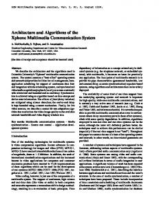
Figure 1.1: SOC Design Complexity Trends [7]

Figure 1.1 illustrates the SoC design complexity trends made by International Technology Road-map for Semiconductors 2011 (ITRS) [7]. ITRS predicts that the number of Processing Engines will grow rapidly in subsequent years to reach the 6000 PEs by 2026. Also, the amount of main memory is assumed to increase proportionally with the number of Processing Elements (PEs). In the same way, the number of Data Processing Engines (DPEs) will increase significantly, leading to more than 70 TFlops processing performance [7]. As the number of cores keeps increasing, and in order to efficiently take advantage of this large number, specific constraints must be taken into consideration. For example, design complexity, low energy dissipation, small silicon area, manufacturer and yield, resource management, etc.. In particular, the interconnection network

1.1. Background

3

starts to play a more and more important role in determining the performance and also the power consumption of the entire chip [8]. Interconnects consume more than 50% of dynamic power, and this percentage is expected to increase [9]. Those factors made conventional shared-bus and Point-to-Point (P2P) systems no longer reliable architectures for SoCs, due to the lack of scalability and parallelism integration, high latency and power dissipation, and low throughput. Figure 1.2 (a) and Fig.1.2 (b) show shared-bus and P2P interconnects, respectively.

(a)

(b)

Figure 1.2: Conventional SoC architectures: (a) Shared-bus, (b) Point-2-Point

1.1.2

Network-on-Chips

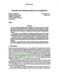
Network-on-Chips (NoCs) [10, 12–18] were introduced as a promising method which can respond to the issues mentioned above. Based on a simple and scalable architecture platform, NoC connects processors, memory, and other custom designs together using switching packets on a hop-by-hop basis in order to provide a higher bandwidth and more enhanced performance. As shown in Fig.1.3, NoC architectures are based upon connecting segment (or wires) and switching blocks to combine the benefits of the two previous architectures while solving their disadvantages, such as the large numbers of long wires in P2P and the lack of scalability in shared-bus systems.

1.1. Background

4

Figure 1.3: Network-on-Chip architecture

NoC main components Observing Fig.1.3, we can distinguish three main components in a given NoC system: • Routers: Routers, labeled R in Fig.1.3, handle the transfer of packets between each other in a hop-by-hop fashion until they arrive to their destination. They are considered as the backbone of any NoC architecture. This is because they perform the routing, switching, and flow-control functions to establish a correct packet transfer between a given source and destination pair. These functions will be discussed in details in the next chapter. • Links: Links provide the connection between the different routers and allow the exchange of data between them. Links can be bi- or uni-directional, or they can contain several physical or logical channels. They may also be pipelined to enhance the system overall performance. This depends on the target application and its performance requirements that need to be satisfied. • Network-Interface (NI): Usually, NIs constitute the sole medium interface between Processing Elements (PE) and routers. As the communication protocol

1.1. Background

5

between these two components is different, NIs handle the conversion of data coming from the PE (for example, Load instruction) into the NoC format represented in packets or flits. NIs’ functions may be extended to satisfy some parameter constraints. For example, when the data coming from the PE exceeds the link capacity (due to a limited hardware budget), NIs may handle the packetization of this data into small packets. When they arrive to their destination node, these packets are assembled to their initial data state in the attached NI. This process is known as depacketization. With this property, reducing the number of links can be achieved (thus, reducing the area and power overhead) while making sure that the performance remains unchanged. In addition, using a Network-Interface allows hiding the implementation details of the communication structure. This means that the network have no information about the attached PE, and vice versa. Challenges At the same time, future applications are getting more and more complex, demanding a good architecture to ensure a sufficient bandwidth for any transaction between memories and cores as well as communication between different cores on the same chip. All of these factors made NoC not enough reliable for future systems, especially when we talk about hundreds and thousands of cores. This limitation comes basically from the high diameter that NoC suffers from. The network’s diameter is the number of hops that a flit traverses in the longest possible minimal path between a (source, destination) pair. The diameter is an important parameter for the NoC design since a large network diameter has a negative impact on the worst case routing latency in the network. For all these facts, the seek for optimizing NoC-based architectures becomes more and more necessary. A lot of research have been conducted to achieve this goal in various approaches, such as: developing fast routers [19–22] or designing new network topologies [23–25].

1.2. Problems and Motivation

1.1.3

6

3D-Network-on-Chips

One of the proposed solutions to enhance the performance of NoC systems and alleviate their limitations, was evolving it to the third dimension. In the past decade, 3-Dimensional Integrated Circuits (3D-ICs) [26, 27] have attracted a lot of attention as a potential solution to resolve the interconnect bottleneck. A 3-dimensional chip is a stack of multiple device layers with direct vertical interconnects tunneling through them [28, 29]. The research made so far have shown that 3D-ICs can achieve higher packing density due to the addition of a third dimension to the conventional two-dimensional layout; and thanks to the reduced average interconnect length, 3D-ICs can achieve higher performance. Besides that, with this reduction of total wiring a lower interconnect-power consumption can be obtained [30, 31]. Not forget to mention that circuitry is more immune to noise with 3D-ICs [27]. This may offer an opportunity to continue performance improvement using CMOS process with smaller form factors, higher integration density, and supporting the realization of mixed-technology chips [32]. As Topol et al. in [31] stated, 3D-ICs can improve the system performance even in absence of scalability. Combining the NoC structure with the benefits of the 3D integration leads us to present 3D-NoC as a new architecture. This architecture responds to the scaling demands for future SoC, exploiting the short vertical links between the adjacent layers that can clearly enhance the system performance. This combination may provide a new horizon for NoC designs to satisfy the high requirements of future large scale applications.

1.2

Problems and Motivation

As 3D-NoC architectures started to show their outperformance and energy efficiency against 2D-NoC systems, questions about their reliability to sustain their performance growth begun to arise [33]. This is mainly due to challenges inherited from both 3D-ICs and NoCs: On one side, the complex nature of 3D-IC fabrics and the continuing shrinkage of semiconductor components. Furthermore, the significant heterogeneity in 3D chips which are likely to mix logic layers with memory layers and

1.3. Thesis objectives and contributions

7

even more complex technologies increases the fault’s probability in a system [34]. On the other side, the single-point-failure nature of NoCs introduces a big concern to their reliability as they are the sole communication medium. As a result, 3D-NoC systems are becoming susceptible to a variety of faults caused by crosstalk [36], impact of radiations [37], oxide breakdown [100], and so on [126]. A simple failure in a single transistor caused by one of these factors may compromise the entire system reliability where the failure can be illustrated in corrupted message delivery, time requirements unsatisfactory, or even sometimes the entire system collapse. In fact, it is predicted that on a future 100-billion transistor chip, 20-billion transistors will be malmanufactured and further 10-billion will fail during operation [35]. This forecast might be pessimistic; nevertheless, it is evident that the failure rate is going to substantially increase in future CMOS technologies [37–39]. To ensure reliability, 3D-NoC systems should be able to detect first the fault occurrence then working on reconfiguring the system resources to recover from these faults and guarantee the continuous correct functionality of the system. Detection can be obtained by relying on custom testing mechanisms or other detection scheme based on codes. Codes are largely used in NoC systems and they were proposed to detect and correct errors in specific components of the system at the presence of a specific type of fault. For instance, Crosstalk Avoidance Codes (CAC) [40, 41] are used for transmission wires and they are considered more efficient than the already existing methods (e.g., shielding [42]) to avoid crosstalk. For errors whose presence could not be detected, Error Detection Codes (EDC) and Error Correcting Codes (ECC) [43] are used to detect and correct these errors. Checking mechanisms in 3D-NoC systems are out of the scoop of this thesis and we are mainly interested in correcting the faults detected by reconfiguring the system components to recover from these faults.

1.3

Thesis objectives and contributions

Starting from all the facts mentioned above, in this thesis we propose 3D-FaultTolerant-OASIS (3D-FTO), a reliable fault-tolerant 3D-NoC system endorsed with

1.3. Thesis objectives and contributions

8

efficient routing algorithms. The proposed system is leveraging on adaptive resource allocation to handle a large number of transient, intermittent, and permanent faults. Along the thesis, we show the ability of the proposed techniques to be easily adopted to any kind of topology, switching policy, flow control, or detection mechanisms. The main contributions of this research are: • Routing: To address link faults, graceful fault-tolerant routing algorithms are proposed: – We first present an efficient fault-tolerant routing algorithm, named LookAhead-Fault-Tolerant (LAFT) [11], to mitigate the different kinds of link faults. LAFT takes advantage of look-ahead routing to boost the performance of 3D-NoCs while ensuring link fault-tolerance and minimizing the additional hardware. Moreover, when errors cannot be contained in a single router (entire input-buffer or crossbar is declared faulty), LAFT is invoked to declare the router as faulty, then reconfigured to bypass it to avoid any information loss. – We present later a second routing that deals with LAFT’s weakpoints. We called this optimized routing algorithm Hybrid-Look-Ahead-FaultTolerant (HLAFT) [10]. HLAFT combines both local and look-ahead routing to further enhance the router’s throughput under worst-case fault scenarios and make the performance degradation as graceful as possible. • Reliable router architecture relying on adaptive resource allocation to the most susceptible components to faults with redundant resources to insure faulttolerance: – Input-buffer: To encounter these faults, a smart buffering mechanism, named Random-Access-Buffer (RAB) [10, 44, 45], was firstly introduced for deadlock-recovery. RAB was also extended and endorsed with TrafficPrediction-Unit (TPU) to tolerate faults in the input-buffer slots. – Crossbar: We employed Bypass-Link-on-Demand (BLoD) [45] approach that provides the appropriate and minimal bypass channels as alternative

1.4. Thesis outline

9

escapes whenever crossbar channels are detected faulty. • Evaluation: The proposed architecture was synthesized using Synopsys Design Compiler with 45nm CMOS process and evaluated with different parallel benchmarks and traffic patterns. Evaluation results and analysis are provided to show the benefits gained with the proposed architecture.

1.4

Thesis outline

The rest of the thesis is organized as follows: • In Chapter 2, we first overview on-chip interconnect main components and we highlight the ones that are proper to 3D-NoC systems. Later, we present the different types of faults in NoC systems and their main causes. • Chapter 3 presents some of the important previously conducted work that dealt with fault-tolerance in NoC systems. We focus mainly on routing algorithms targeting the link failure in 3D-NoC systems, and also works presenting reliable router architectures presented for 2D-NoC architectures, but can be adopted in the third dimension. • Chapter 4 is dedicated to the fault-tolerant routing algorithms proposed in this thesis to solve the link failure. We start first by presenting Look-AheadFault-Tolerant (LAFT) routing and we show its benefits. Then we explain how we can further optimize LAFT by combining both look-ahead and local routing for better routing decision making. The optimized routing algorithm is named Hybrid-Look-Ahead-Fault-Tolerant routing algorithm (HLAFT). • Chapter 5 introduces the proposed 3D-FTO router architecture and its main components. We start first by presenting a brief overview of the baseline 3D-OASIS-NoC router. Second, we introduce Random-Access-Buffer (RAB) mechanism and its efficiency to recover from deadlock and also to tackle the failure problem in input-buffers. Third, the Traffic-Prediction-Unit (TPU) that we proposed for further traffic balance and reduce the buffer congestion

1.4. Thesis outline

10

is also explained. Finally, we explain Bypass-Link-on-Demand (BLoD) aimed to ensure fault-tolerance in the crossbar. • We dedicate Chapter 6 for the evaluation methodology and results. We describe the different adopted benchmarks and assumed parameters, then we provide a comprehensive evaluation and analysis of the different techniques and algorithms proposed in this thesis. • Finally in Chapter 7, we end this thesis with the conclusion. We also discuss how this work can be optimized furtherer.

Chapter 2 On-Chip Interconnects and Reliability In this chapter, we introduce the on-chip interconnect paradigm and we explain its main components including topology, switching policy, flow-control, and routing algorithms. We also highlight the transition from 2D- to 3D-NoC including the necessary modifications in addition to the parameters that are proper to 3D-NoC systems. Moreover, we state the main advantages and challenges of these latter systems. Finally, we present the different types of faults in NoC systems and their main causes.

2.1

Overview of on-Chip interconnect

The on-Chip interconnection is characterized by several components and parameters. The selection of each one of these is based on some reasons and backgrounds regarding the fulfillment of the bandwidth requirements for specific applications and parallel computing applications as well. NoC systems can be implemented using different topologies, forwarding methods, flow controls, routing algorithms, and so on. The understanding of these categories is primordial before starting the design phase. Since each type of this technique has its own characteristics and impacts on the system overall performance. In this section, we explain the importance of each one of these keywords and we present the different types of each one of them. 11

2.1. Overview of on-Chip interconnect

2.1.1

12

Topology

The topology defines the way routers and links are interconnected. Topology is an important design choice as it defines the communication distance and its uniformity. Some of the most used topologies are depicted in Fig. 2.1. The choice of a topology depends on its advantages and drawbacks [46, 47]. Usually, regular topologies (Fig. 2.1 (a-e)) are preferred over irregular ones (Fig. 2.1 (f)), because of their scalability and reusable pattern. Otherwise, irregular or mixed topologies can be more conveniently adapted to specific needs of the application. This depends on the target application which may require some area, power, or timing constraints that need to be strictly satisfied. In this case, regular topologies might not be the right approach to implement such special applications, and custom irregular ones offer better flexibility to meet the desired requirements. On the other hand, one of the main problems that irregular topologies suffer from is the design time needed to profile the application and decide the best topology layout that satisfies these design requirements. The Mesh [48, 49] and Torus [50] based topologies are considered as the most commonly used on-chip network topologies. Together they constitute over 60% of 2D-NOC topology cases [51]. Mesh and Torus are depicted in Figs. 2.1 (a) and (b), respectively. Both of them can have four neighboring connections; but, only Torus has wraparound links connecting the nodes on network edges. Other topologies like Butterfly, Fat-tree, and Ring (depicted in Figs. 2.1 (c), (d) and (e), respectively) have roughly even proportions. Compared with other on-chip network topologies, the mesh topology in particular can achieve better application scalability. The implementation of routing functions in mesh topology is also simpler and can be characterized well. In the on-chip interconnection networks for on-chip multiprocessor systems, the mesh architecture is widely used and preferable. An example of on-chip multiprocessor system that uses mesh topology is Intel-Teraflops system [52]. The 80 homogeneous computing elements are interconnected through NoC routers in the 2D mesh 8×10 network topology.

13

Figure 2.1: NoC topologies.



2.1.2

14

Forwarding methods

There exist two kinds of forwarding methods in NoC interconnects: 1) circuit switching and 2) packet switching. In the first method, the path between a given source and destination pair should be firstly established and reserved before starting to send the actual data. This offers some performance guarantees as the message is sure to be transferred to its destination without the need for buffering, repeating, or regenerating. Moreover, if during the establishment of the path a problem is detected (such as failure or high congestion), the source node can recompute another safer path to be reserved again. However, the path setup required for each message increases the latency overhead, in addition to the extra congestion caused by the different control data traveling the network and competing with the actual data for the network resources. Therefore, it is best suited for predictable transfers that are long enough to amortize the setup latency. Packet-switching is more common and it is utilized in about 80% of the studied NoCs [51]. In packet switching, routers communicate through transmitting packets/flits through the network. The transmission of a given packet should not block the communication of other ones in the network. To solve this problem, a forwarding method (switching policy) can be selected to define how the network resources (link and switched) are reserved and how they are torn down after the transfer completion. The forwarding methods have a big impact on the NoC performance and each one of them has its advantages and drawbacks. In packet switching, Store-and-Forward (SF), Wormhole Switching (WH), and Virtual-Cut-Through (VCT) are considered as the main switching methods [53]. Store-and-Forward (SF) switching In this switching method, each message should be divided into several packets. As depicted in Fig. 2.2, each packet is completely stored in a First-In-First-Out (FIFO) buffer before it is forwarded into the next router. Therefore, the size (depth) of FIFO buffers in the router is set similar to the size of the packet in order to be able to completely store the packet. This represents the main drawback of this switching policy since it requires a significant amount of buffer resources which increases as


15

Figure 2.2: Store-and-Forward switching.

we increase the packet size. This amount of allocated buffer slots has a huge impact on the area and power consumption of the NoC system. Moreover, as can be seen in Fig. 2.2, node (0,2) has two empty slots since the first two flits of Packet-4 (P4F1 and P4F2) have been already transmitted. Despite the available two slots, Packet-5 (P5) in node (0,1) is still stalled. This is because in order to be forwarded, all the four slots in node (0,2) should be freed; therefore, P5 can be forwarded only when P4 is forwarded as well and the buffer slots are freed. Store-and-Forward was the first switching method that has been used in many parallel machines [54–56]. It was also in the first prototypes and designs of NoC [57–61]. Wormhole (WH) switching Wormhole switching (WH) is one of the most popular, well-used, and well suited for NoC systems. In WH switching method, represented in Fig. 2.3, packets are divided into a number of flits. As can be seen in Fig. 2.3, the four flits of Packet-1


16

Figure 2.3: Wormhole switching.

(P1F1, P1F2, P1F3, and P1F4) are dispersed in four different routers. Therefore, no need for buffer resources to host the entire packet. The main advantage of the wormhole switching is that the buffer size can be set as small as possible to reduce the buffering area cost. This responds to the area and power overhead of SF. However, blocking is one of its major drawbacks. As depicted in Fig. 2.3, the last flit of P1 is located at the head of the south input-buffer of node (1,0). At the tail of the same input-buffer, the first flit of Packet-2 (P2) is requesting the grant to be forwarded to the north output-port (heading for node (2,0)). In this scenario, there is a tight dependency between the first P1F4 and the second P2F1. In other words, if P1F4 is forwarded then P2F1 can be forwarded as well; however, in case where P1F4 is blocked for congestion or failure reasons in the downstream nodes, then P2F1 is blocked too. Consequently, the remaining flits of P2 and the dependent other flits will be blocked as well. This will lead to the partial or entire system deadlock and a significant performance degradation. One of the solutions to solve this problem in


17

Figure 2.4: Virtual-Cut-Through switching.

WH switching is the use Virtual-channels [62]. This is discusses later in this chapter (Section 2.1.5). The wormhole switching method was firstly introduced in [63]. The work in [64] has presented also the performance of the wormhole switching in k-ary n-cube interconnection networks. Virtual-Cut-Through (VCT) switching Figure 2.4 demonstrates Virtual-Cut-Through (VCT) switching. VCT is an intermediate forwarding method that has the properties of both SF and WH. As represented in 2.4, with VCT it is possible to forward flits one after another. So, flits from different packets can share the same input-buffer eliminating the stalling caused by SF. In order to solve the blocking problem found in WH switching, VCT requires that the buffer depth should be equal to the packet size (number of flits in the packet). This buffer size is needed to store blocked flits. When blocking happens, flits are stored in a router next to the blocked one. The buffer size is larger than


18

Figure 2.5: ON/OFF flow control.

WH switching since the entire packet is stored. However, the forwarding latency is much smaller than SF switching. This is because in the Store-and-Forward packet switching method the packet is completely stored before it is forwarded to the next router and the delay to wait for the complete packet storing is very long.

2.1.3

Flow control

Flow control determines how resources, such as buffers and channels bandwidth are allocated, and how packet collisions are resolved [16]. Whenever the packet is buffered, blocked, dropped, or misrouted, this depends on the flow control strategy. A good flow control strategy should avoid channel congestion while reducing the latency. ON/OFF, Credit-based, and ACK/NACK are commonly used control flows used in NoC [13] and are explained in this subsection. ON/OFF flow control ON/OFF flow control [65] has protocols which can manage data flow from upstream routers while issuing a minimal amount of control signals. It is able to do this because it has only two states: ON or OFF. This control flow has threshold values, which are dependent on the number of free buffers in downstream routers.


19

Figure 2.6: Credit-based flow control.

The threshold values are used to decide the states of the control signals. When the number of free buffers is over the threshold, downstream routers emit an OFF signal to upstream routers, stopping the flow of flits. Meanwhile, downstream routers send flits to other nodes, and the number of free buffers becomes less than the threshold value. At that time, downstream routers emit an ON signal to upstream routers, restarting the flow of flits. Since the ON/OFF signals are just sent to switches only, there is a low calculation time. Figure 2.5 indicates one transmission example with ON/OFF flow control. Credit-based flow control In Credit-based flow control (CB) [13, 16, 66, 67], upstream nodes have information about the number of empty slots in downstream buffers. We call this information CN (Credit Number). Each time an upstream node sends a flit to downstream buffers, the number is decremented by one. When downstream buffers send some flits to other nodes, they also send a credit control signal to upstream routers, and when the upstream router receives the signal, the CN associated with the path is incremented appropriately. Figure 2.6 illustrates the data flow and an example of transmission. In this example, initially Router 2 is blocked, and CN is decremented.


20

Figure 2.7: ACK/NACK flow control.

Next Router 2 starts sending flits and credit signals are emitted to Router 1, which receives the signal and re-starts sending flits to Router 2. ACK/NACK flow control The above flow controls send signals from the downstream buffers to upstream ones and decide whether or not to send flits. On the other hand, ACK/NACK flow control [13, 65] does not need to wait and calculate such signals from downstream buffers. In this flow control model, as flits are sent from source to destination, a copy is kept in each of the node buffers to resend it, if necessary, in case where some flits are dropped. An ACK signal is sent from a downstream node when a flit is received. When the upstream node receives this signal, it deletes its copy from its buffers. If the downstream node cannot or does not receive the correct flits, it sends NACK signal to the upstream node, and the upstream node rewinds its output queue and starts resending a copy of the corrupted flit. 2.7 depicts an example of this flow control.


2.1.4

21

Routing algorithms

This subsection presents some basic backgrounds and concept about routing algorithms. In general, the selected routing algorithm for a network is topology dependent. This section will give only a brief description about routing algorithms and their taxonomy. Routing algorithms can be classified according to several criteria [68]: • Number of destinations: According to the number of destination nodes, to which packets will be routed, routing algorithms can be classified into unicast routing and multicast routing as shown in 2.8. The unicast routing sends the packets from a single source node to single a destination node. The multicast routing sends the packets from a single node to multiple destination nodes. The multicast routing algorithm can be divided further into Tree-based multicast routing and Path-based multicast routing.

Figure 2.8: Categorization of routing algorithms according to the number of destinations: (a) unicast, (b) multicast.

• Routing decision locality: According to the place where the routing decisions are made, routing algorithms (unicast or multicast routing) can be classified into source routing and distributed routing. As depicted in 2.9, in the distributed routing, there will be one header probe (for unicast routing case)


22

Figure 2.9: Categorization of routing algorithms according to decision locality: (a) distributed, (b) source.

containing the address of the destination node (the source node address can be also embedded). The routing information is locally computed each time the header probe enters a switch node. In the source routing, paths are computed at the source node. The pre-computed routing information for every intermediate node, to where a message will travel, will be written in a routing probe. All routing probes that represent the routing paths from the source to destination node will then be assembled as packet headers for the message. • Adaptivity: In all cases of the routing implementation seen so far, the routing algorithm can be either deterministic or adaptive (as represented in 2.10). In deterministic routing, the computed paths from a source and destination pair are statically computed and will always be similar. In adaptive routing algorithms, the paths from source to destination can be different, because the adaptive routing selects adaptively the alternative output ports. An output channel is selected based on the congestion information or the channel status of the alternative output ports. Adaptive routing algorithms generally guide messages away from congested or faulty regions in the network and they can be further classified according to the number of alternative adaptive turns as


Figure 2.10:

23

Categorization of routing algorithms according to adaptivity: (a)

deterministic, (b) adaptive.

Fully adaptive and Partially adaptive routing algorithms. • Minimality: According to the minimality of the routing path, routing algorithms can be classified into minimal or non-minimal algorithm (see Fig. 2.11). The minimal adaptive routing algorithm will not allow a message to move away from its destination node. In other words, the message will always be routed closer to its destination node traversing the minimal number of hops to reach its destination. In the non-minimal algorithm, the message can be routed away from its destination node. This can be performed randomly or following some rules and restrictions usually found in adaptive routing algorithms.

2.1.5

Deadlock and Livelock

Deadlock Deadlock is caused by the cyclic dependency between packets in the network. It is one of the major issues in NoC systems which is caused when packets in different


Figure 2.11:

24

Categorization of routing algorithms according to minimality: (a)

minimal, (b) non-minimal.

buffers are unable to progress because they are dependent on each other forming a dependency cycle. It can occur because packets are allowed to make all turns in clock-wise and counter clock-wise turn directions. Figure 2.12 illustrates a deadlock example in an adaptive NoC system. The dependency is caused by the flits exchange between R02 and R01 . Due to the presence of faults, the choices for a minimal routing is limited and both communications are dependent on each other; thus, none of them can make progress along the network. On the same figure, we can see that flits Dest10 and Dest00, stored in the input-ports of R11 and R01 respectively, are victims of this deadlock; i.e., even their outputchannels are free, they have to wait in the buffer until the blocking is resolved. Virtual-Channel (VC) [62] is one of the most well used techniques for deadlock avoidance. As illustrated in Fig. 2.13, VC divides the input-buffer in smaller queues which are independent on each other and managed by an arbiter. When a blockage happens in one VC, the other ones are not affected and they continue asking requests for their corresponding output-channels. In this fashion, non-blocked requests are served and their slots are freed to host other incoming flits. Another technique used for deadlock-avoidance is called Virtual-Output-Queue (VOQ) [69]. In VOQ, as shown in Fig. 2.14, the input-buffer is divided into different


Figure 2.12: Deadlock example in adaptive NoC systems.

Figure 2.13: Virtual-Channel-based router architecture.

25


26

queues to host incoming flits which are stored depending on their corresponding output-channel; i.e., VOQ (i,j) stores flits coming from input-port i wishing to access output-port j. For each output-channel, a 7x1 crossbar(i) is dedicated to handle the traversal of flits coming from the different input-channels and asking the grant for the output-channel(j). According to [70], VOQ can achieve less switch delay than VC with the same efficiency.

Figure 2.14: Virtual-Output-Queue-based router architecture. Both VC and VOQ ensure deadlock-freedom; however, the employment of such techniques is costly in terms of hardware and implementation complexity. This is caused by the arbitration needed to handle the different requests coming from the multiple VCs/VOQs at each input-port. To solve this overhead, another solution for deadlock avoidance can be achieved by applying allowed turns and prohibiting one turn in every clock-wise and counter clock-wise turn direction. The prohibited turns will avoid cyclic dependency between packets in the network. Some routing

2.2. 3D-Network-on-Chip

27

algorithms are solving the deadlock problem based on these prohibitions which are called turn models. The design of adaptive routing algorithms based on turn models has been introduced in [71]. The work has presented examples of turn models for adaptive routing algorithms in 2D mesh-based interconnection network. Livelock If the packets are allowed to make non-minimal adaptive routing, then a problem called livelock configuration may occur. The livelock is a situation where a packet moves around a destination node but it never reaches the destination node. The livelock can be avoided by only allowing the packets to make minimal routings; however, if the non-minimal routing is allowed, then a mechanism to detect livelock must be implemented.

2.2

3D-Network-on-Chip

3D-Network-on-Chip (3D-NoC), is a natural evolution of 2D-NoC. As depicted in Fig. 2.15, the simplest way is to add two additional ports to a given 2D-NoC router for the vertical up and down directions. As in 2D-NoCs, 3D-NoCs are characterized by several components and parameters that designers should carefully decide. Some of them are the same as in conventional 2D-NoCs. This includes the flow control, switching policy, arbitration mechanism, and other methodologies that do not strongly depend on the architecture whether it is 2D or 3D. However, other components and parameters are different when we move to the third dimension. Therefore, in this section we give an attention to these components and methods to better understand the challenges and advantages of 3D-NoC.

2.2.1

Topology and router architecture

3D-NoC is a widely studied research topic and many works have been conducted so far to solve the various challenges in 3D-NoC designs. Few of these works focused on the router architecture and how to ensure the vertical connection between routers from different layers. For example, Li et al. [73] has modified the 7x7 Symmetric 3D


28

Figure 2.15: 4x4x4 3D-NoC mesh topology. router [72] by using a dTDMA bus (distributed Time Division Multiple Access) as a communication interface between the different layers of the network, to create a 3D NoC-Bus Hybrid architecture, as shown in Fig. 2.16. This kind of architectures reduces the number of ports in each router from 7 to 6. However, flits wishing to travel from one layer to another should compete the access to the shared bus, since it is the only inter-layer communication medium. Besides that, to travel from one layer to another each packet should undergo two buffers (one output buffer in the upstream node, then an input buffer in the downstream node). This may increase the dynamic power consumption, in addition to the static power and latency overhead


29

caused by the deployment of the output buffer. All these reasons may lead to undesirable performance degradation especially under a heavy inter-layer traffic.

Figure 2.16: 3x3x3 3D-NoC Bus Hybrid topology [74]. Kim et al. [75], also proposed another structure for the 3D-router called TrueNoC. By implementing all the vertical links into a single 3D-crossbar, the router has only 5 ports since we do not need any more additional ports for the vertical connections. An optimized architecture of True-NoC has been introduced and named 3D Dimensionally-Decomposed (DimDe) [75]. DimDe provides a good tradeoff between circuit complexity and performance benefits presenting consistently the lowest latency [75]. In fact, both systems present promising results by reducing the interlayer distance, and making the travel between the different layers in one single hop possible. But, this kind of routers also dramatically increases the arbiter cost and power consumption, besides the implementation complexity of such structure. Ramanujam et al. [76] considered the load balancing in 3D-NoC and presented a layer-multiplexed 3D design for vertical communication. The main drawback of this architecture is the two-stage crossbar that every flit should traverse which is considered as non-efficient in terms of power. Park et al. [77], presented a MultiLayered On-Chip Interconnect Router Architecture (MIRA) that implements a 2D mesh multiprocessor-chip in the third dimension. However, with such technique the processor cores are assumed to be designed in 3D which makes existing highly optimized 2D processor cores difficult to be reused. Matsutani et al. [78] introduced XNoTs. This architecture requires large vertical links which makes it a less power efficient solution.


2.2.2

30

Routing algorithms

Another important design challenge that should be taken care of while designing a 3D-NoC is the routing algorithm. Many routing algorithms have been proposed for NoC systems but most of them focused only on 2D-NoC topologies. Among all the studies conducted for 3D-NoCs, few of them targeted routing algorithms and they can be classified into two categories. The first one includes some of the well known routing schemes in 2D-NoC that were extended to the third dimension, such as Dimension Ordered Routing (DOR) [79], Valiant [80], ROMM [81], O1TURN [82]. The routing algorithms in the second category are specially proposed for 3DNoC architectures including some custom routing schemes that aim to balance the traffic along the network or to reduce the thermal power. For instance, Ramanujam et al. [83] presented an oblivious routing algorithm called Randomized Partially Minimal (RPM) that targets balancing the traffic along the network, improving then the worst case scenario. RPM sends packets to a random layer first, then routes them along their X and Y dimensions using either XY or YX routing with equal probability. Finally, packets are sent to their final destination along the Z dimension. In a quite similar technique, Chao et al. [84] addressed the thermal power problem in 3D-NoCs. Starting from the fact that the upper layers in the network detain the highest thermal power of the design, they proposed a thermal aware downward routing scheme that sends first the traffic to a downer layer, routes along the X and Y dimensions before sending the packets back up to their destination node. This technique avoids communication in upper layers, where the thermal power is more important than the downer ones, and then can ensure the thermal safety of the design.

2.2.3

Through Silicon Via (TSV)

Contrary to horizontal links in 2D-NoC, 3D NoC vertical links consist in bundles of Through Silicon Vias (TSVs) [85,86]. Represented in Fig. 2.17, a TSV is a vertical connection which is made into silicon. The positive side of TSVs is that it enables vertical interconnections, and allows the stacking of different dies. This enables the


31

reduction of the chip footprint, and at the same time improves the performance due to the vertical interconnections. We highlight in the next two paragraphs the size and placement challenges of TSVs and their important role in defining the reliability of 3D-NoC systems.

Figure 2.17: TSV channel in a 3D Wafer Level Packaging [87].

TSV Dimensions A TSV can have different diameters and different pitch. As depicted in Fig. 2.18, the pitch is the required distance between two given TSVs. The diameter and the pitch have a strong relationship. The smaller the diameter is, the smaller the pitch, and the denser the design. The problem with TSVs is that it cannot shrink the same way like transistors do. This is why TSVs are far bigger than transistors. One of the reasons the TSV cannot be shrunk under a certain size is if the diameter of a TSV is shrunk, the wafer thickness should also be smaller, because of via filling reasons [86]. [86] states that when using TSVs with diameters of 10 nm and less, the density can go as high as 10000 TSV/mm2. Nevertheless, very small diameter TSVs have been designed where 4 nm wide TSV have been patterned with lithography using 3.2 µm thick photo-resist [88].


32

Figure 2.18: 3x3 TSV array. Placement The placement of TSVs on a chip determines the reliability and speed. For example, a regular placement of TSVs improves the exposure quality of the lithographic process and therefore improves the yield [90]. On the other hand, the keep-out-zone (KOZ) (as shown in Fig. 2.18) is an area outside of the TSV, where no transistor can be placed because of reliability issues. But, because of this, the pitch of the TSVs becomes larger, so does the area which will be covered by TSVs and KOZ. Authors in [89] compare several TSV placement topologies, and states that area and performance wise, the shielded and isolated topologies are preferred.

2.2.4

3D-NoC advantages and challenges

3D-NoC systems inherit several advantages from the 3D-Integration. We can summarize them as follow: • Footprint: More functionalities fit into a smaller space and the device density increases. This extends Moore’s Law and enables a new generation of tiny but powerful devices. • Speed: The average wire length becomes much shorter with 3D-NoC, and


33

since the propagation delay is proportional to the square of the wire length, the overall performance is enhanced and the bandwidth is increased compared to System-in-Package (SiP). • Power: 3D-NoCs offer two features that contribute in the power reduction: 1) keeping the signals on-chip (and not off-chip) which reduces the power consumption by ten to a hundred times [91], 2) and also by reducing the wire length, power consumption can be also decreased by producing less parasitic capacitance. • Heterogeneous integration: Circuit layers can be built with different processes, or even on different types of wafers. This means that components can be optimized to a much greater degree than if they were built together on a single wafer. Even more interesting, components with completely incompatible manufacturing could be combined in a single device [92], enabling new features. Despite the advantages mentioned above which are promising to open several new possibilities for new, secure and flexible design possibilities, 3D-NoCs are facing several challenges: • Yield: Each extra manufacturing step (layer thinning, TSV creation, bonding) adds a supplementary risk for defects: misalignment, dislocation, void formation, oxide film formation over copper interfaces, pad detaching, defects due to temperature, coupling and so on. In addition, the accumulated effects of these defects are very difficult to predict and prevent. • Heat: Thermal buildup within the stack must be prevented or dissipated. Different solutions have been proposed, including thermal TSVs [93]. • Design complexity: Taking full advantage of 3D requires intricate and elegant multi-level designs. Chip designers will need new CAD tools to address the 3D paradigm [94]. This has an important effect on the time-to-market as it is an important constraint.

2.3. Reliability in on-chip interconnect

34

• TSV footprint: The footprint of a vertical link is huge with respect to the 2D counterparts, because of the very large TSV diameter and pitch (tens of mm [95, 96]).

2.3

Reliability in on-chip interconnect

Faults can occur at any component of a 3D-NoC system (i.e., link, router, buffers, crossbar, and so on). Their rates of occurrence, reasons, and places depend on the design, technology, environment and operation conditions.

2.3.1

Reliability and time

From a time perspective, the duration of faults is paramount especially for realtime 3D-NoC systems and it can be categorized into three main types [97]: 1) Transient faults: they occur and remain in the system for a particular period of time before disappearing; 2) Intermittent faults: they are transient faults that occur from time to time; 3) Permanent faults: they start at a particular time and remain in the system until they are repaired.

2.3.2

Failure and main factors

The three types of faults can be caused by several internal or external factors. While previous works presented in details the different failure mechanisms [126], we just briefly highlight below some of the most well-known and well-studied faults: Transistor Infant Mortality (TIM) [98]: This failure is a direct result of the continuing shrinkage of the transistor dimensions shrinkage. This makes the manufacturing of transistors quite complex and the early transistor failure is more often to happen. Burn-in is one of the processes that most of the manufacturers use to quickly eliminate the weakest and most vulnerable transistors by applying high voltage and temperature. By the end of this process, only components possessing robust transistors will survive. However, this process is starting to lose its efficiency in nanometer technology scaling due to the increased temperature leading to leakage

2.3. Reliability in on-chip interconnect

35

current which leads to yet higher increasing temperature. As a result, aggressive burn-in will destroy even robust transistors. Electromigration (EM) [99]: EM is caused by the diffusion of metal atoms along the conductor in the direction of electron flow. This happens when the metal conductor gets smaller and, in consequence, its current density increases. Therefore, the ions in the conductor start to migrate leaving holes in the metals. As a result, some regions of built up unwanted metal can short to an adjacent trace. Time Dependent Dielectric Breakdown (TDDB) [100]: TDDB occurs when the thin Oxide insulator between the gate and the induced channel begins to wearout by time. The main consequence for this phenomenon is the formation of a conducting path through the Oxide to the substrate. At the presence of such path, a leakage current through the Oxide to the substrate starts to flow. As the technology allowed the Oxide to be thinner and thinner, TDDB is one of the main concerns of manufacturers and ASIC designers. Hot carrier degradation (HCD) [101]: the presence of a strong electrical field causes the carriers to heat-up. This heat causes the transistor transconductance to slowly degrade and the threshold voltage to change. With threshold voltage shifted, some parts of the circuit do not meet their time requirements leading to time faults or in some cases the entire device may encounter failure. Process variation (PV) [102]: PV is one of the common concerns resulted from the evolution of technology and manufacturing process. The continuous variation of transistor dimensions and doping concentration leads to increasing concerns, as well as higher possibility for low performance devices. Single-Event Upset (SEU) [103]: SEU is a logic glitch and a main factor that may cause the wrong computation of a given combinational logic. Despite the fact that many earlier works tried to diminish the importance of such failures and that many major manufacturers assure that the problem is solved in their products, SEU still remain a big concern especially due to the growing chip density and reduced supply voltage.

2.4. Conclusion

2.3.3

36

Reliability and locality

From a locality perspective, it is important to analyze the behavior of faults in the different components of the system to find the ones where the faults are more often to occur. According to [143], input-buffers and crossbar occupy the largest area in 3D-NoC system that can reach the 80% and 10%, respectively. While each one of the remaining components do not pass the 3% of the router total area. Consuming the largest portion of the router area, the fault occurrence probability is very high in the input-buffers and crossbar if we assume that the faults’ distribution is proportional to the area distribution. Therefore, adopting fault-tolerance for inter-router links (as in most 3D-NoC systems) is not enough to build a reliable system, and faults’ consideration should also include the buffers and crossbar.

2.4

Conclusion

In this chapter, we presented the key components and parameters of NoC systems including topology, switching policy, flow-control, and routing algorithms. We demonstrated their different categories and their corresponding effects on the performance of a given NoC. We also introduced the additional components needed for the transition from 2D- to 3D-NoC. We focused mainly on the necessary modifications and parameters that are proper to 3D-NoC system (i.e., Through-Silicon-Vias) in addition to the advantages and drawbacks of these systems. At the end of this chapter, we analyzed the different types of faults that NoC systems are vulnerable to and how they can be classified regarding time and locality. In the next chapter, we focus on how prior works tried to solve the failure issue in on-chip interconnect.

Chapter 3 Related Work to Fault-Tolerant Techniques in NoCs In this chapter, we discuss some of the important related work that dealt with fault-tolerance in NoC systems. We focus mainly on routing algorithms targeting the link failure in 3D-NoC systems, and also works presenting reliable router architectures presented for 2D-NoC designs, but can be adopted in the third dimension.

3.1

Fault-tolerant solutions for 2D-NoC systems

Many works have been conducted so far to tackle fault-tolerance in NoC systems where they can be classified depending on the target system, the fault’s type, or the faults’ handling mechanism (e.g., using routing algorithms or architectural solutions). The majority of the fault-tolerant solutions were proposed for 2D-NoC systems. Some of them added restrictions to the number of faults as a security requirement for their systems. For instance, a single link or single node failure tolerance was presented in [104]. Gomez et al. [105] presented a solution that can handle five failures with the aid of Virtual channels (VCs). For n-dimensional mesh, Duato et al. [106] presented a routing algorithm that can tolerate up to n-1 faults. Another part of the proposed solutions eliminated the number of faults restriction and, instead, they limited the location of faults to a specific part of the network. They called these restricted subnetworks fault-regions which can be disabled, if nec37

3.2. Fault-tolerant solutions for 3D-NoC systems

38

essary, to ensure fault-tolerance of the system. These restrictions can be represented by the shape of the fault-regions (convex [107], rectangular [108], or polygon [109]), their locations (excluding faults located at the edges of the network [110]), or assuming the absence of faults in some specific parts of the router (datapath [111], links and crossbar [112]). Some works were presented without adding any restriction to either number of faults or locations. For example, uLBDR [113] routing for 2D mesh topology based on Virtual-cut-through which incurs a high complexity despite its great performance. Works in [114, 115] are based on stochastic approaches to tolerate transient and permanent faults. In another adaptive routing algorithm, named Immunet [116], packets use a reserved VC as an escape channel to reach their destination and avoid a faulty link. Other works [118, 119] focused on the importance of adopting minimal routing algorithms to reduce the congestion caused by the presence of faults. They proposed minimal routing schemes that are able to adaptively route packets through the shortest paths, as long as a path exists. Authors in [117], presented a comprehensive investigation about 2D/3D fault-tolerant routing algorithms’ implementation. They discussed the different turn models, fault conditions, and the fault occurrence in both links and routers.

3.2 3.2.1

Fault-tolerant solutions for 3D-NoC systems Fault-tolerant routing algorithms

Due to the important negative impact of faults on 3D-NoCs system performance, implementing fault aware techniques is extremely important to avoid any component or entire system failure. In this direction, some of the proposed fault-tolerant solutions for 3D-NoC systems primarily focused on permanent faults occurring in Through-Silicon-Vias (TSVs). For example, Loi et al. [127] addressed the TSV yield improvement by presenting a solution based on spare via insertion. Pasricha et al. [128] introduced serialization to achieve also the same goal. On-chip sequential elements protection techniques were also proposed in [129, 130] to deal with single


39

event upsets. The other existing works for 3D-NoC systems focused on link failure in general by adopting fault-tolerant routing algorithms. For example, Rahmani et al. [131] presented a fault-tolerant routing algorithm for named AdaptiveZ targeted for Hybrid3D-NoC architecture. Feng et al. [121] proposed a low overhead deflection routing algorithm based on routing tables. However, the deployment of routing tables is still costly in terms of hardware and suffers from poor scalability due to the area required for the tables. Nordbotten et al. [132] presented an adaptive and fault-tolerant routing for 3D meshes and tori based on storing at each node a table for routing containing information about destination and the list of intermediate nodes. A fault-tolerant routing algorithm for 3D torus was presented by Yamin et al. [133]. With up to 30% faulty-node rate, the proposed algorithm can find a valid link between two faulty nodes with a probability higher than 90%. The Planar Adaptive Routing (PAR) for large scale 3D topologies was introduced by Chien et al. [134] who used three virtual channels (VC) for deadlock avoidance and employed also some routing rules. Wu et al. [120, 135] extended this scheme to adopt at least four VCs to avoid deadlock. In [136] a fault model based on PAR, named 3D minimum-connected component (MCC), was presented. Each fault-free node needs to store four copies of safety information, one for each subnet. Later, Xiang et al. [137] proved that, despite the advantages obtained when compared to PAR, MCC may mislead a packet to a dead end, and they claimed that their proposed fault model, named planar network (PN), needs to store much less safety information at each faulty-free node (PN needs to keep 16-bit safety information and 32-bit for 3D MCC [137]). The problem with the solutions mentioned above is that they introduce an extremely expensive hardware complexity and implementation cost besides the energy overhead making them undesirable for the 3D-NoC implementation. In another work, Feng et al. [121] proposed a low overhead deflection routing algorithm based on routing tables. They proposed a routing table for each 2DMesh layer, and two TSV state vectors for the vertical links. In fact, this solution reduces the area overhead, when compared to Global Routing table [122]. However,


40

the deployment of routing tables is still costly in terms of hardware and suffers from poor scalability due to the area required for the tables. Pasricha et al. [138] extended a 2D turn model for partially adaptive routing to the third dimension. The proposed scheme combines both 4N-FIRST and 4P-FIRST schemes to propose a lightweight 4NP-FIRST. On the other hand, this turn model introduces some routing restriction to prevent from deadlock. These restrictions cause a nonminimal routing selection where in some cases it may take too many additional hops for the packet to reach its destination, even when a nonfaulty minimal path exists. This has a negative effect on the zero-load latency and also the dynamic power consumption due to the increasing number of hops. To ensure a minimal path for flits while considering link faults, Wu et al. [123] presented an adaptive and minimal routing algorithm based on limited-global safety information. Despite the merits of such technique, the main problem of this proposal is that the algorithm is based on faulty node model (and not faulty link). This means that many working parts or nodes are disabled even if they have nonfaulty links that can be used. A recent work by Akbari et al. [139] focused mainly on faults links and proposed an algorithm named AFRA. This algorithm routes packets through ZXY in the absence of link faults. When faults are detected, the algorithm switches the routing to XZXY: The flits are sent first to an escape node through X, and then they continue to their destination through ZXY as it is in the no-fault case. The authors presented simplicity, good performance and robustness as the main features of this algorithm. However, we complement this solution due to two major aspects. First, AFRA tolerates only vertical links and horizontal links are not taken into consideration. Second, the network congestion status is not taken into consideration, especially when more than one possible minimal path is available. In that case, a static minimal path selection does not eventually lead to low latency (i.e. a minimal path may contain a high congestion while other alternative ones do not). Ebrahimi et al. [124] stated that AFRA requires a fault distribution mechanism to know about the fault information on all vertical links along each row. They proposed a more reliable routing algorithm named HamFA which does not require any fault distribution, additional fault information, or any virtual channels. They


41

modified the basic form of the Hamiltonian path in order to be able to switch between high and low channel subnetworks. In fact, HamFA provides much more reliability than AFRA; however, it requires that the faulty links should belong to the same subnetwork in order to tolerate multiple vertical or horizontal one-faulty links. As a result, this limits the reliability of this approach to 95% when considering the presence of a single faulty link. In our approach, no restrictions are added to the fault locations and they can be anywhere in the network as long as there exists a valid path between a given (source, destination) pair.

3.2.2

Router architecture solutions

In this subsection, we focus on the earlier conducted works which tried to address the fault issue in the router level. Constantinides et al. [140] proposed the BulletProof router which is based on N-modular redundancy (NMR) technique to ensure fault tolerance. The NMR method requires the presence of N copies of a given targeted component. Thus, N times extra silicon area is needed; therefore, such method is very expensive in terms of area. Moreover, as the area increases the fault occurrence probability increases, as well. As a result, duplicating components may not lead to endorse the reliability. Kim et al. [141] proposed RoCo that employs decoupled parallel arbiters and uses smaller crossbars for row and column connections in order to allow the router to be decomposed. Look-ahead routing is used to tolerate faults in the Routing Computation stage (RC). By sharing arbiters from Virtual Channel Allocation stage (VCA), fault tolerance in the Switch Allocation stage (SA) can be ensured. However, this router cannot tolerate faults in VCA and Crossbar Traversal (CT) stages where the area is more important and faults are more likely to occur in these stages. Poluri et al. [142] presented an improved router design where they added a small minimal correction circuitry to provide a better fault-tolerance in each one of the pipeline stages. The proposed router adds a redundant routing computation unit in each input-port to ensure fault-tolerance in the RC stage. With the help of some extra state fields in the input port, a faulty VC can use the arbiter of another VC that belongs to the same input-port. To solve the fault occurrence in the SA


42

stage, they created a bypass path at the presence of faulty arbiters. Finally for the CT stage, they proposed to have two paths to reach a particular output-port of the crossbar. Evaluation results showed the outperformance of their proposed router. They also claimed that the proposed router provides higher reliability when compared to earlier works. However, they do not consider the presence of faults in the input buffer. As we stated earlier, buffers consume the largest portion of area and power; therefore the probability of fault occurrence is the highest when compared to the other components of the router. An interesting work was proposed by DeOrio et al. [143] targeting permanent faults. They presented a reliable architecture based on resource redundancy reconfiguration endorsed with a distributed routing algorithm. They proposed flexible-fifo to deal with permanent faults in the input-buffers by indexing the tail and head pointers through redirection-table that manages to increment (or decrement) the head (or tail) counter multiple times before accessing the next functional register, thereby skipping over failed registers [143]. To deal with faults in the crossbar, they introduced Crossbar-Bypass-Bus that provides an alternative path when a faulty crossbar link is detected. The proposed architecture by DeOrio et al. showed great results under various topologies and different fault-rates; however, it has three main drawbacks. First, this architecture deals with only permanent faults and does not consider transient and intermittent faults. As Lehtonen et al. stated in [144], transient faults cause the majority of failures (80%), while the rest of them originate mainly in permanent and intermittent faults. On the other hand, this should not diminish the importance of permanent faults; thus, analyzing the three types of failures is imperative to represent the real behavior of 3D-NoC systems. The second drawback is that when multiple faulty crossbar paths are detected, flits from different input-ports should compete the access for this single bypass-bus. This puts under question the scalability of this approach when the latency may increase at the presence of more than one faulty crossbar link. Third, the companion routing protocol contains some restrictions and turns to ensure the system deadlock-freedom; however, and as we previously said, the addition of such rules may lead to nonminimal path, thus,

3.3. Conclusion

43

increasing the latency of the flit. The main motivation of this work is to enhance the performance of our baseline 2D-OASIS-NoC architecture by taking advantage of the high performance and energy efficiency of 3D-NoC system. Initially as a stepping stone, an exploration of the design issues in Gigascale NoC architectures was presented in [16]. The first OASIS-NoC system was then presented in [125] which uses deterministic XY routing, wormhole switching, a First-Come, First-Served (FCFS) scheduler, and re-transmission flow control which is like ACK/NACK flow control. Later, OASIS-2 system [17] was introduced to optimize the earlier one. With the aid of Matrix-arbitration scheduler, Stall-Go flow control, and Look-ahead-XY, OASIS-2 showed better performance then the earlier one. To solve the high diameter of 2D-NoC, in [18] we presented ONoC-SPL that establishes a Short-Pass-Link (SPL) to reduce the communication latency for performance enhancement in data-intensive computation applications. ONoC-SPL showed great performance compared to the previous designs; however, it is still not scalable enough for large systems. Therefore, we opted for threedimensional NoC and presented 3D-OASIS-NoC in [162] which is a natural extension of the baseline 2D-OASIS-NoC. In [145, 146] we introduced Look-Ahead-XYZ (LAXYZ) which reduces the router delay to increase the system throughput.

3.3

Conclusion

In this chapter, we discussed some of the important related work that dealt with fault-tolerance in NoC systems. Mainly routing algorithms have been investigated, especially those targeting the link failure in 3D-NoC systems. In addition, we reviewed the works presenting reliable router architectures presented for 2D-NoC architecture, but can be adopted in the third dimension. At the end of this chapter, we showed the different steps conducted in this work starting from the building stone OASIS-NoC system arriving to 3D-OASIS-NoC which is considered as the baseline design in this thesis. Despite the encouraging results obtained with the baseline 3D-OASIS-NoC, it

3.3. Conclusion

44

still does not support fault tolerance which makes it vulnerable to any risk of false calculation, information loss, timing violation, or the entire system failure. In the next two chapters, we present the different algorithms and techniques that we propose to ensure fault-tolerance at low cost and without considerable performance degradation.

Chapter 4 Efficient Fault-tolerant Routing Algorithms for Robust Architectures This chapter focuses on the routing algorithms proposed in this thesis. We start first by presenting an overview of the Look-Ahead-XYZ routing algorithm that our baseline 3D-OASIS-NoC router uses. This aims to provide a comprehensive discussion on the benefits of look-ahead routing and the reasons why we want to take advantage of it. Second, we explain our first proposed Look-Ahead-Fault-Tolerant routing (LAFT) routing algorithm. We demonstrate its key features and advantages and discuss its weakpoints. In the last section, we propose the optimized and second algorithm Hybrid-Look-Ahead-Fault-Tolerant routing (HLAFT) algorithm that deals with its predecessor’s drawbacks.

4.1

Look-Ahead-XYZ Routing Algorithm Overview

Conventional XYZ routing [79, 84, 159, 160] compares the address of the processing node with the destination node’s address to determine the Output-Port. The computed information is sent to the Switch-Arbiter requesting access of the selected output-port. Despite its simplicity, XYZ suffers from an inefficient pipeline stage usage [22, 161], which can incur a high communication latency and, therefore, de45

4.1. Look-Ahead-XYZ Routing Algorithm Overview

46

grading the system throughput [147].

Figure 4.1: Conventional XYZ routing router pipeline stages. Figure 4.1 shows a conventional router pipeline design based on the XYZ scheme. Virtual Channels are not taken into consideration for improving the performance of best-effort traffic. This figure shows the router’s four pipeline stages: Buffer Writing (BW), Routing Calculation (RC), Switch Arbitration (SA), and the Crossbar Traversal stage (CT). This router’s design increases the flit latency because any flit should go through all these stages at each hop while traveling from source to destination [22, 161]. This can introduce undesirable overall system performance degradation, especially with a large network size where the network diameter scales [20]. In these routing algorithms, the pipeline stages are dependent on each other, and each one of them cannot perform its computation unless it receives information from the previous stage. This dependency is especially seen between the RC and SA stages. To solve this dependency problem, Look-Ahead-XYZ (LA-XYZ) parallelizes the RC, now referred as Next-Port-Calculation stage NPC, and SA stages and eliminates the dependency between them [145, 146]. To avoid any confusion, it is important to mention that the NPC stage with LA-XYZ plays the same role as of RC in conventional routing. The difference is RC calculates the output-port for the current node, and NPC calculates the output-port for the next downstream node as explained later. LA-XYZ precomputes the Next-Port direction of the downstream router and then embeds it in the flit [146]. When arriving to the downstream node, this hot encoded Next-Port identifier will be used by the Switch-Arbiter directly to request authorization for using the selected output-port and reaching the next neighboring node. At the same time, when the grant is computed in SA, the RC calculates in

4.2. Look-Ahead-Fault-Tolerant routing algorithm

47

parallel the direction of the Next-Port that will be used by the next downstream node. This parallel process optimizes the pipeline stages as shown in Fig. 4.2. LA-XYZ computation goes under two steps: Assign next address and Define new Next-port. The first step decodes the Next-Port identifier from the incoming flit. Depending on the direction of this identifier, the address of the next downstream node can be computed. This address is then used in the second step by comparing it with the destination address of the flit, which is also fetched from the flit’s head. At the end of this process, information about the Next-Port is issued and embedded again in the flit to be used as a source of information for the Switch-Arbiter in the downstream node.

Figure 4.2: Look-Ahead-XYZ routing router pipeline stages. LA-XYZ’s lack of support of fault tolerance outweighs the performance merits obtained when compared to other 3D routings (XYZ [79] and RPM [83]) [145, 146]. In addition, it suffers from a low worst-case throughput since the network congestion is not considered in the routing decision process.

4.2 4.2.1

Look-Ahead-Fault-Tolerant routing algorithm Assumptions

To keep the benefits of the look-ahead routing, the proposed Look-Ahead-FaultTolerant (LAFT) performs the routing decision for the next node taking into consideration its link status and selects the best minimal path. Before starting to explain LAFT, there are two important assumptions that should be mentioned. First, the links connecting the PE to the local input and output ports are always nonfaulty.


48

Second, we assume that there exists at least one minimal path between a (source, destination) pair. These assumptions are natural and necessary to deliver any flit from source to destination.

4.2.2

Fault detection

We employed a simple fault detection mechanism based on a single multiplexer in each input-port that reads the incoming flit and verifies whether it is corrupted or not. Depending on this verification, the Fault-Control-Module (FCM) sends a single-bit signal to the upstream node that can be either 0 or 1, for valid or faulty, respectively, as shown in Fig. 4.3 (Details about FCM will be provided in the next chapter). Each router sends the collected information corresponding to its own fault status to each one of the six neighboring nodes and also to the Network-Interface of the attached PE (see Fig. 4.3). This information is represented in a 6-bit signal representing the router link status in each direction (North, East, Up, South, West, and Down). It is important to mention that the choice of using control signals to transfer the fault information rather than using control flits is taken to enhance the performance. Using the latter approach will increase the congestion in the router, where we may find data and control flits competing for the router resources.

4.2.3

Algorithm

The fault information is read by each input-port where LAFT is executed. Algorithm 1 illustrates LAFT algorithm. The first phase of this algorithm calculates the next node address depending on the next-port identifier read from the flit. This phase is the same as in LA-XYZ. For a given node wishing to send a flit to a given destination, there exist at most three possible directions through X, Y, and Z dimensions, respectively. In the second phase, LAFT performs the calculation of these three directions by comparing x, y and z coordinates of both current and destination nodes concurrently.

49

Figure 4.3: Fault information exchange.



50

At the same time, as these directions are being computed, the fault-control module reads the next-port identifier from the flit and sends the appropriate fault information to the corresponding input-port. By the end of this second phase, LAFT has information about the next node fault status and also the three possible directions for a minimal routing. In the next phase, the routing selection is performed. Algorithm 1: Look-Ahead-Fault-Tolerant routing algorithm (LAFT) // Destination address Input: Xdest , Ydest , Zdest // Current node address Input: Xcur , Ycur , Zcur // Next-port identifier Input: Next-port // Link status information Input: Fault-in // New-next-port for next node Output: New-next-port // Calculate the next-node address Next← Next-node (Xcur , Ycur , Zcur , Next-port); // Read fault information for the next-node Next-fault← Next-status (Fault-in, Next-port); // Calculate the three possible directions for the next-node Next-dir← poss-dir (Xdest , Ydest , Zdest , N extx , N exty , N extz ); // Evaluate the diversity number of three minimal paths Div1 ← path-div (Xdest , Ydest , Zdest , poss − dir1 ); Div2 ← path-div (Xdest , Ydest , Zdest , poss − dir2 ); Div3 ← path-div (Xdest , Ydest , Zdest , poss − dir3 ); // Evaluate the New-next-port direction if (|Next-dir| > 1) then if (Div1 ==Div2 ==Div3 ) then New-next-port ← min-congestion (poss − dir1 , poss − dir2 , poss − dir3 ); else New-next-port ← max-diversity (poss − dir1 , poss − dir2 , poss − dir3 ); end else if (Next-dir == 1) then New-next-port← N ext − dir1 ; else New-next-port← nonminimal (Xdest , Ydest , Zdest , Xcur , Ycur , Zcur , Fault-in); end

For this decision, we adopted a set of prioritized conditions to ensure fault tolerance and high performance either in the presence or absence of faults: 1. The selected direction should ensure a minimal path, and it is given the highest


51

priority in the routing selection. 2. We should select the direction with the largest next hope path diversity. 3. The congestion status is given the lowest priority. Depending on these priorities, LAFT reads the fault status of the next node received from the fault-control module and checks the number of possible nonfaulty minimal directions. As illustrated in algorithm 1, if only one nonfaulty minimal direction is obtained, this direction will be selected as out-port for the next node. If more than one possible minimal direction is available, the algorithm selects the direction that leads to a node with higher path diversity. The diversity value for a given node is the number of possible directions leading to the destination through a minimal path. A node with high diversity results in more routing choices. This means that the probability of finding a nonfaulty link is greater when considering faults. When no faults are detected in the system, selecting the direction with the highest diversity gives more choices to find the least congested direction. As stated in [138], to obtain directions with high diversity, we should select those leading to nodes located in the center of the mesh and avoid routing to the edges of the network. When the three possible directions are minimal and have the same diversity, the routing selection is made depending on the congestion of each output port. This congestion information is obtained by the stop signal issued from the flow control used in our 3D-OASIS-NoC system. When there is no valid minimal route available, LAFT chooses a nonminimal route while also considering the 2nd and 3rd priorities (path diversity and congestion) as illustrated in algorithm 1.

4.2.4

Example

To understand better how LAFT works, we observe Fig. 4.4. Assuming that the current node (labeled C) received an incoming flit where the next port identifier, calculated in the previous node, indicates that the out-port for this flit is East (Red arrow). Applying algorithm 1, the next node address is calculated (labeled N). Three minimal directions are possible for routing: East, North, or Up. The East direction will not be selected since the link in this direction is faulty.

Figure 4.4: Look Ahead Fault Tolerant routing algorithm example.

4.2. Look-Ahead-Fault-Tolerant routing algorithm 52


53

Therefore, either North or Up can be selected, which both are minimal and nonfaulty. In this case, the diversity priority is taken into consideration. If Up is selected, where the node in this direction is on one of the network edges, the diversity value is equal to 2 (two minimal possible directions: East or North). However if North is selected, its diversity value is equal to 3 (East, North, or Up). Having the highest priority, the North out-port (Green arrow) is selected for the next node and it is embedded in the flit to be used in the downstream node to allow the routing calculation and switch allocation to be performed both in parallel. As long as the chosen route is minimal, the livelock problem does not exist either. However, it can be observed when a nonminimal direction is selected. For this reason, some restrictions are added when selecting the nonminimal route in addition to the one mentioned above. The first restriction forbids the flit to turn back to the same direction where it came from. The second one forbids selecting a path that is in the opposite direction of the faulty link (i.e., if ”East” is faulty, then ”West” should not be selected). Adopting these restrictions guarantees the livelock freedom of LAFT, and the flits will continue to advance and search for a route until it finds a valid link. The deadlock problem may arise with LAFT. This problem is solved thanks to the proposed Random-Access-Buffer mechanism (RAB) that we discuss in the next chapter.

4.2.5

Weakpoints

Employing look-ahead routing reduces the router latency and improves the system overall performance [11]. However, due to the limited information restricted to only one switch ahead, in some cases LAFT may not select the best route. Observing the example in Fig. 4.5 (a), we can see that the North route is leading to a blocked path where all the minimal possible directions to the destination are faulty. Therefore, nonminimal routing is required causing several additional clock cycles. When arriving to the next node (labeled N), the out-port is already decided and sent to the Switch-allocator due to the look-ahead routing restraints. This is despite the fact that this path is leading to a blocking path and also a better blocking-free route exists (Up).

Figure 4.5: Example of fault-tolerant routing: (a) Look-ahead routing (LAFT) (b) Hybrid routing (HLAFT).

4.2. Look-Ahead-Fault-Tolerant routing algorithm 54

4.3. Hybrid-Look-Ahead-Fault-Tolerant routing algorithm

55

Optimizing LAFT and making it able to detect whether the route precalculated in the previous upstream node would lead to a blocked path or not is necessary. To enable this, the benefits of look-ahead routing should be combined with local routing for better routing selection.

4.3

Hybrid-Look-Ahead-Fault-Tolerant routing algorithm

The new Hybrid-Look-Ahead-Fault-Tolerant routing algorithm (HLAFT) solves the earlier mentioned problems of LAFT [10]. At every incoming flit, HLAFT makes a simple computation to judge whether the precalculated Next-port identifier will lead to a blocking path or not. In case where a possible nonminimal route might occur, HLAFT recomputes the route depending on the local and neighboring nodes fault status.

4.3.1

Algorithm

Algorithm 2 represents the new HLAFT routing. At first, the fault-control module at each input-port reads the Next-port identifier and destination addresses from the flit. Depending on the Next-port value, the next-node can be calculated. After acquiring information about the next-node, the three possible minimal directions are computed and checked whether a valid minimal route leading to the destination exists or not. In case where at least a valid minimal link leading to the destination exits, the Next-port identifier is sent to the Switch-allocator and the look-aheadrouting-computation (LA-RC) modules at the same time. In the opposite case (i.e., all the possible three directions are faulty), a flag is issued triggering the localrouting-calculation module (Loc-RC) to recalculate the output-port by verifying the status of the current and neighboring nodes links. The same three priorities, earlier explained in the previous subsection (i.e., minimal valid, higher diversity, and less congested), are taken into consideration while selecting the new out-port. The recalculated out-port issued from Loc-RC is sent to the Switch-allocator to perform

4.3. Hybrid-Look-Ahead-Fault-Tolerant routing algorithm

56

the arbitration, and also sent to the LA-RC module to compute the Next-port for the next-node to continue the look-ahead routing cycle. Algorithm

2:

Hybrid-Look-Ahead-Fault-Tolerant

routing

algorithm

(HLAFT) // Destination address Input: Xdest , Ydest , Zdest // Current node address Input: Xcur , Ycur , Zcur // Next-port identifier Input: Next-port // Link status information Input: Fault-in // New-next-port for next node Output: New-next-port // Calculate the next-node address Next← Next-node (Xcur , Ycur , Zcur , Next-port); // Read fault information for the next-node Next-fault← Next-status (Fault-in, Next-port); // Calculate the three possible directions for the next-node Next-dir← poss-dir (Xdest , Ydest , Zdest , N extx , N exty , N extz ); // Evaluate the flag if (|Next-dir| == 0) then flag← 1; else flag← 0;; // Evaluate the New-next-port if (flag == 1) then // Trigger local-routing out-port← local-routing (Fault-in, Xcur , Ycur , Zcur , Xdest , Ydest , Zdest ); // Execute LAFT with the new recomputed out-port New-next-port← LAFT-routing (Xcur , Ycur , Zcur , Xdest , Ydest , Zdest , out-port, Fault-in); else // Execute LAFT with the inputed Next-port identifier New-next-port ← LAFT-routing (Xcur , Ycur , Zcur , Xdest , Ydest , Zdest , Next-port, Fault-in); end

4.3.2

Example

As illustrated in Fig. 4.5 (b), when the flit arrives to the node labeled C and having a current out-port North precalculated in the previous node, the fault-control checks the fault status of the links of the next-node in the north direction. When performing the checking, all the possible minimal paths are found faulty; thus, Loc-

4.4. Adaptivity

57

RC is triggered and computes Up as the new best route (since East is faulty). Then, the newly calculated Up direction is sent to the LA-RC module which issues North as the Next-out-port.

Figure 4.6: Hybrid-Look-Ahead-Fault-Tolerant routing router pipeline stages. Figure 4.6 depicts the HLAFT pipeline stages which takes advantage of lookahead routing to parallelize both Next-Port-Calculation (NPC) and Switch-Arbitration (SA) stages. We can also observe first that a pipeline stage is dedicated for the fault-control module (FTC) to issue the flag and whether trigger local-routing or not. This simple computation is done in parallel with the Buffer Writing stage (BW) to further reduce the computation latency in the router without creating any critical paths. In case where no flag is issued, the Local-Routing-Calculation stage (LocalRC) is bypassed and then Next-Port-Calculation and Switch-Arbitration stages are performed in parallel (NPC/SA). In the presence of a flag, Local-RC is performed and then the results are sent to NPC/SA stage before the final Crossbar Traversal stage (CT) handles the flit transfer to the next neighboring node.

4.4

Adaptivity

Hybrid-Look-Ahead-Fault-Tolerant routing (HLAFT) showed its efficiency to provide a minimal path while ensuring both fault-tolerance and congestion-aware properties. In this research, the proposed algorithms were implemented on a Meshbased system. However, it is important to say that they are tightly dependent on the mesh topology and it can be easily adopted for other ones, whether regular or irregular. This is because the only portion which is topology-dependent and should be modified in the algorithms is the calculation of the three possible directions for

4.5. Conclusion

58

the next-node, as depicted in algorithm 1. While the remaining parts are not only restricted to the adopted Mesh topology. Therefore, both LAFT and HLAFT are flexible routing algorithms that can be easily altered to fit with any 3D-NoC topology.

4.5

Conclusion

In this chapter, we presented two efficient routing algorithms that aim to tackle the fault occurrence in inter- and intra-layer links. We started by explaining the baseline Look-Ahead-XYZ routing algorithm that our baseline 3D-OASIS-NoC router is based upon. Then, we introduced the first Look-Ahead-Fault-Tolerant routing (LAFT) routing algorithm and we showed its ability to reduce the router latency by exploiting the benefits of look-ahead routing and traffic awareness. As seen in Chapter 6, LAFT shows its ability to reduce the latency by an average of 32% when compared to conventional routing algorithms. More details about LAFT routing algorithm can be seen in [11, 44]. After discussing the weak points of LAFT, we proposed Hybrid-Look-AheadFault-Tolerant routing (HLAFT) algorithm to solve LAFT’s drawbacks. We showed that combining both local and look-ahead routing enhances the path variety and minimizes the probability for nonminimal routing. HLAFT was presented in [10], and from the evaluation results (see Chapter 6) it made the performance degradation further graceful by 12% when compared to LAFT. At the same time, only a small area and power overhead has been observed. The implementation of both LAFT and HLAFT routing algorithms in in Verilog-HDL can be seen in the appendix. Both LAFT and HLAFT have shown their efficiency in dealing with the fault occurrence in inter- intra-layer links. On the other hand, with a large number of cores and layers, 3D-NoC systems face greater challenges and become more vulnerable to faults. At this high core density, considering faults only in the inter-router links does not provide the optimal reliability. Other components such as input-buffers and crossbar should be given greater attention to ensure fault tolerance and enhance the system reliability. These components consume a large portion of the entire

4.5. Conclusion

59

router area and power budget. To this aim, we present in the next chapter different modules added to address the reliability in 3D-NoC systems in order to address the fault occurrence in the input-buffers and the crossbar circuit.

Chapter 5 Reliable Router Architecture and Design for Fault-Tolerant 3D-NoC Systems In this chapter, we introduce the proposed 3D-FTO router architecture and its main components. We start first by presenting a brief overview of the baseline 3DOASIS-NoC router. Second, we introduce Random-Access-Buffer (RAB) mechanism and its efficiency to recover from deadlock and also to tackle the failure problem in input-buffers. The Traffic-Prediction-Unit (TPU) that we proposed for further traffic balance and reduce the buffer congestion is also explained. Next, we explain the Bypass-Link-on-Demand (BLoD) aimed to ensure fault-tolerance in the crossbar. Finally, we dedicate the last subsection to describe the main functionalities of the Fault-Control-Module (FCM) and its important role in orchestrating the different process inside the router.

5.1

3D-OASIS-NoC baseline router architecture overview

The baseline 3D-OASIS-NoC system architecture and the router block diagram with its three main pipeline stages (Buffer Writing, Routing calculation/Switch Ar60

5.1. 3D-OASIS-NoC baseline router architecture overview

61

bitration and the Crossbar Traversal) are represented in Fig.5.1.

5.1.1

Switching method

3D-OASIS-NoC adopts Wormhole-like switching [53]. The forwarding method, chosen in a given instance, depends on the level of the packet fragmentation. For instance, when the buffer size is greater than or equal to the number of flits, VirtualCut-Through is used. However, when the buffer size is less than or equal to the number of flits, Wormhole switching is used. In this way, packet forwarding can be executed in an efficient way while maintaining a small buffer size.

5.1.2

Router architecture

The router is the back-bone component of the 3D-OASIS-NoC design. Each router has a maximum number of 7-input and 7-output ports, where 6 input/output ports are dedicated to the connection to the neighboring routers and one input/output port is used to connect the switch to the local computation tile. The number of input-ports depends on the router position in the network because we need to eliminate any unused ports to reduce the area and power consumption. The 3DOASIS-NoC router contains seven Input-port modules for each direction in addition to the Switch-Allocator and the Crossbar module that handles the transfer of flits to the next neighboring node [162].

5.1.3

Input-port circuit

The Input-port module is shown in Fig.5.2. It is composed of two main elements: Input-buffer and the Route module. Incoming flits from different neighboring routers, or from the connected computation tile, are first stored in the Input-buffer. This step is considered as the first pipeline stage of the flit’s life-cycle BW. Each input-buffer can host up to 4 flits. Figure 5.3 demonstrates the 3D-OASIS-NoC’s flit format. The first bit indicates the tail informing the end of the packet. The next three bits are dedicated to indicate the Next-Port that will be used by the Look Ahead Fault Tolerant routing algorithm to define the direction of the next


Figure 5.1: Baseline 3D-OASIS-NoC system architecture.

62


Figure 5.2: Input-port module architecture.

63


64

downstream neighboring node where the flit will be sent to. Then, three bits are used to store destination information of each xdest, ydest and zdest. Finally, the remaining 64 bits are dedicated to store the payload. Since 3D-OASIS-NoC is targeted for various applications, the payload size can be easily modified in order to satisfy the requirements of some specific applications. In addition, the architecture does not provide a separate head flit and every flit therefore identifies its X, Y, and Z destination addresses and carries an additional single bit to indicate whether it is a tail flit or not.

Figure 5.3: 3D-OASIS-NoC flit format.

Figure 5.4: Switch allocator block diagram. After being stored, the flit is read from the FIFO buffer and advances to the next pipeline stage. The destination addresses (xdest, ydest and zdest) are decoded


65

in order to extract the information about the destination address, in addition to the Next-Port identifier which is pre-calculated in the previous upstream node, and the fault information received from Fault Controller. These values are sent to the Route circuit where LAFT is executed to determine the New-next-Port direction for the next downstream node. At the same time, the Next-Port identifier is also used by the Switch Request Controller to generate the request for the Switch-Allocator asking for permission to use the selected output port via sw-req and port-req signals.

5.1.4

Switch-Allocator circuit

The sw-req and port req signals issued from each Input-port module, and giving information about the desired output-port, are transmitted to the Switch-Allocator module to perform the arbitration between the different requests. This process is done in parallel with the routing computation in the Input-port module to form the second pipeline stage RA/SA. At the end, the Switch-Allocator sends the swcntrl signal that contains all the information needed by the Crossbar circuit about the scheduling result. The latter, forming the last pipeline stage CT, reads the corresponding flit from the granted Input-port and sends it to its allocated outputchannel. The switch allocator module is composed of two main components: StallGo flow control and Matrix Arbiter Scheduling (Fig.5.4). Stall-Go flow control module When the buffer exceeds its flit storage capacity, a flow control has to be considered to prevent buffer overflow and packet dropping. We use Stall-Go flow control for 3D-OASIS-NoC since it proves to be a low-overhead efficient design choice showing remarkable performance compared to the other flow control schemes such as ACK-NACK or Credit based flow control [65]. Stall-Go module, whose mechanism is represented in Fig.5.5, uses two control signals: nearly-full and data-sent. Nearlyfull signal is sent to the downstream node to indicate that the buffer is almost full and only one slot is available to host one last flit. After receiving this signal, the FIFO buffer suspends sending flits. The data-sent signal is issued when the flit is transmitted informing that one slot in the buffer is released.

Figure 5.5: 3D-OASIS-NoC flow control mechanism.


66

5.2. Proposed 3D-Fault-Tolerant-OASIS-NoC router architecture

67

Matrix arbiter Scheduling module The switch allocator in our design employs a least recently served priority scheme [17]. Thus, it can treat each communication as a partially fixed transmission latency [148, 149]. Matrix-arbiter is used for a least recently served priority scheme. In order to adopt the Matrix-arbiter scheduling for 3D-OASIS-NoC, we implemented a 6x6 scheduling-matrix for each output-port. The scheduling module accepts all the requests from each of the different connected input-ports and their desired outputports before assigning a priority for each request. The scheduling module verifies the scheduling-matrix, compares the priorities of the different requests, and grants access to the one possessing the highest priority. The scheduling module updates the matrix with the new priorities of each request to ensure that every input-port will be served in a fair way. Complete details about the baseline 3D-OASIS-NoC architecture and comprehensive evaluation results can be fond in [150].

5.2

Proposed 3D-Fault-Tolerant-OASIS-NoC router architecture

Figure 5.6 depicts the high-level representation of 3D-Fault-Tolerant-OASIS (3DFTO) baseline router (in white) in addition to the enhancement added (colored) for fault-tolerance and robustness enhancement. 3D-FTO router relies on simple detection and recovery techniques based on system reconfiguration with redundant structural resources to contain faults’ occurrence (in input-buffers, crossbar, and links) and prevent from the system failure, or information corruption or loss. As shown in Fig.5.6, 3D-FTO router contains seven input-ports, a switch-allocator, a crossbar, and a Fault-Control-Module (FCM). In this section, we explain the enhancements added in 3D-FTO router including, first, the Random-Access-Buffer (RAB) for deadlock-recovery and fault-tolerance with the help of the Traffic-PredictionUnit (TPU) in the input-buffer. Second, the Bypass-Link-on-Demand (BLoD) approach to handle multiple faulty channels in the crossbar.

Figure 5.6: 3D-OASIS-NoC router architecture.


68


69

Finally, the FCM module responsible for the assignment and control of the different detection and recovery tasks to the previously mentioned techniques.

5.2.1

Random-Access-Buffer mechanism

Deadlock-recovery As is the case for every adaptive routing algorithm, the deadlock issue may rise. As we previously mentioned in Section 1, most of the existing routing algorithms use either Virtual-channels (VCs) or add restrictions to the routing selection to avoid deadlock. These solutions either suffer from high implementation complexity or incur an additional delay due to the nonminimal approach. In our case, we implemented a similar technique to VCs, but it is much simpler and less complex. This technique, named Random-Access-Buffer (RAB), detects first the flit being the reason of deadlock in the buffer, drops its request and then looks for another flit whose request can be granted to free some slots in the buffer and break the dependency. Random-Access-Buffer for deadlock-recovery architecture Figure 5.7 shows an example how RAB works. In each input-port, a buffer-controller (BC) manages the detection of deadlock and handles the assignment of wr-adr and rd-adr addresses. The detection mechanism is based on a timer which after a period of time, if the request being processed is not served, a flag is issued informing the presence of a deadlock (Fig. 5.7 (a)). This is done by reading the sw-grnt signal received from the Switch-allocator. In this case, the BC reads the head of the next packet in the buffer and checks whether the requested out-port is different from the one previously flagged as blocked or not. When it finds a request whose channel is free (Fig. 5.7 (b)), it sends a request to the Switch-allocator to be served. When the request is granted, the flits of the granted packet are read from the buffer and the freed slots can be used to host another incoming packet (Fig. 5.7 (c)). After new flits are written in the buffer, the blocked packet is checked again (Fig. 5.7 (d)). The BC receives a grant for the direction requested (North) and the packet is read from the buffer.

(d)

(c)

Figure 5.7: Example of deadlock-recovery with Random-Access-Buffer.

(b)

(a)

5.2. Proposed 3D-Fault-Tolerant-OASIS-NoC router architecture 70


71

The timer’s value is one of the important choices that should be carefully taken. This is because the deadlock occurrence is strongly dependent on the application for any adaptive routing algorithm. Moreover, the presence of faults in the system adds a higher probability for the deadlock occurrence; therefore, before selecting the value of the timer, we profiled each one of the used applications and analyzed the task graph of each one of them. During this analysis we took into consideration the fault-rate and its impact on the congestion and deadlock occurrence. Overwriting avoidance mechanism In order to avoid any flit overwriting caused by mismanaging the wr-adr and rd-adr addresses, we added a small status register (SR) which keeps information about the flits being flagged (i.e., not served yet). When a flit is read from the buffer, the BC checks the status register and makes sure not to write the incoming flit in a flagged slot. Observing, Figs. 5.7 (a) and (b), we can see that status[0] and status[1], which are keeping information about the two flits of the flagged packet are updated to 1. As shown in Fig. 5.7 (c), when an incoming flit arrives to the buffer, BC makes sure that it will not be stored in one of these two flits’ locations, but instead it is stored in an empty one. When a flit which was previously flagged, and after of period of time its request is granted, the BC should update the status register to free the flagged slot so it can be used by other incoming flits, as it is show in Fig. 5.7 (d) (status[0] is updated to 0). With this simple technique, performance and deadlock-freedom are ensured while guaranteeing a small overhead. Moreover, instead of managing many requests at the same time, as it is the case of VCs requiring then additional complexity and delay for the arbitration, RAB handles each request at a time. Despite the delay penalty required by the timer to detect the deadlock, this technique is still faster and simpler to implement than Virtual-channels. Power management For the proposed system, we used a power management scheme to reduce the dynamic power in the system. This scheme is based on clockgating to turn-off the clock in some specific components which, in some periods of time, they are in a waiting state and not performing any computation. Therefore, it is important to switch off these components when they are not necessary for the


72

correct working of the system and they are awakened when the system requires their services.

Figure 5.8: Random-Access-Buffer for deadlock recovery block diagram. We employed the power management scheme in three main components. First, when a router detects that one of its links is faulty, it immediately switches off the clock from the entire input-port associated to this faulty link. In this case, an important amount of dynamic power can be saved since input-ports occupy the largest portion of the system power budget due to the presence of buffers which are considered as the hungriest components in the entire system in terms of power. Second, we turn off the clock in the local-routing module that we added to recompute the incoming route if necessary. Thus, the local-routing module is initially not fed by the clock. Whenever the fault-control module signals the necessity to recompute the route, the local-routing module is awakened and performs the necessary computation. Otherwise, it is disconnected from the clock and the unnecessary dynamic power is spared. Finally, the last component is the RAB circuit. As we previously mentioned, RAB deadlock-recovery technique is triggered only at the presence of deadlock. When no blocking happens, the buffer is managed by the conventional


73

First-In-First-Out (FIFO) buffer controller, as shown in Fig. 5.8. For dynamicpower saving, RAB is put asleep at the absence of deadlock (deadlock-flag is equal to zero) and it is working only when the timer (deadlock-flag) informs it that deadlock is occurring. In this fashion, deadlock-recovery is insured at a low-cost with no unnecessary power waste. Fault-tolerance RAB was extended to be able to detect transient, intermittent, and permanent faults in the input-buffer. For the detection we assume the presence of a module (fault-detect in Fig. 5.9) that checks the buffer slots fault-status. In fact, the proposed 3D-FTO system including the different techniques is independent of the fault-detection mechanism that can be adopted. As long as the fault-tolerant modules in the router receive information about the presence and locations of the faults, they can efficiently and adaptively recover from them. Therefore, whether we use error detection codes (such as, Error-Detection-Codes (EDC), Error-Correcting-Codes (ECC), Cyclic-Redundancy-Check (CRC), and so on) or specific modules to detect errors, such as Built-In-Self-Test (BIST), 3D-FTO can efficiently handle this fault information regardless of the adopted detection mechanism. When a fault is detected in one of the buffer slots, it can send one of two signals: (1) Int-Tr-faulty-slot to inform the RAB-manager module the presence of a transient or intermittent fault. When receiving this signal, the RAB-manager will take into consideration the flagged slots when assigning Wr-adr and Rd-adr addresses. These two latter signals are very important since they define the locations of the read and written flit that are computed according to the fault status of the buffer slots. At the same time, the RAB-manager keeps checking the flagged slots whether their faults were recovered or not. This is because the buffer contains temporary faults that can disappear after a period of time. (2) In case where a permanent fault is detected, the fault-detect module sends a Perm-faulty-slot signal to the RAB-manager. This information is important because if the RAB-manager finds that only one buffer slot is nonfaulty, and the remaining ones are permanently faulty, it sends a Faulty-buffer signal to the Fault-control-module to disable the entire input-port and update the


74

Link-status array (shown in Fig. 5.6). As we can see here, the distinction between the two Int-Tr-faulty-slot and Permfaulty-slot signals is extremely important to the behavior of the RAB-manager. Depending on which signal is received, the RAB-manager is able to decide whether to avoid writing/reading to/from a buffer slot since the detected faults are temporary and can stop to exist after a period of time, or to disable the entire input-port since the buffer contains permanent faults that cannot be recovered. By disabling the entire port, fault-tolerance can be achieved (i.e., we make sure that the stored information is correct). Moreover, the power overhead of this faulty buffer can be also alleviated, since it is no longer functional and there is no need for powering it on. Optimized status-register To keep record of the faulty slots, the status register (SR), previously presented for deadlock-recovery, was extended to an array that hosts n 2-bit items (where n is the buffer depth). The value of each item can be 00 to inform that the corresponding flit is not causing the deadlock and the buffer slot is not faulty. 01 indicates that the buffer slot is not faulty but the request of the hosted flit is causing deadlock; therefore, this slot can be consulted again to check whether the deadlock is removed or not, but it cannot be used to store incoming flits to avoid flit overwriting. An element in the status array is updated to 10, if a transient or intermittent fault is detected in the corresponding buffer slot. Then, the slot cannot either consulted or used to store incoming flits (to avoid additional latency for consulting broken slots). Finally, 11 is used to declare that the corresponding slot is permanently faulty. As we previously said, these information will be used to issue the Faulty-buffer signal. In addition to the timer, the RAB mechanism is triggered by the fault-detect module where in case of transient or intermittent is removed from a given slot, the fault-detect informs the RAB-manager to update the status array of the corresponding slot to 00 so it can be used by other incoming flits. Example Figure 5.10 shows an example how the RAB mechanism works. In each input-port, a RAB-controller (RAB-cntrl) manages the detection of deadlock


75

Figure 5.9: Random-Access-Buffer for deadlock recovery and fault-tolerance block diagram.


76

(a)

(b)

(c) Figure 5.10: Example of Random-Access-Buffer mechanism for deadlock-recovery and fault-tolerance. Red crosses represent permanent faults, and the green one represents intermittent or transient faults


77

and faults and handles the proper assignment of wr-adr and rd-adr addresses. In Fig. 5.10 (a), and after a permanent fault was detected (red cross) in one of the buffer slots, RAB-manager updates the corresponding element in the status array to 11. Furthermore, by reading the sw-grnt signal received from the Switch-allocator, the timer issues a deadlock-flag and the RAB-manager updates the corresponding slot to 01. The RAB-cntrl reads the head of the next packet in the buffer and checks whether the requested out-port is different from the one previously flagged as blocked or not. When it finds a request whose channel is free, it sends a request to the Switch-allocator to be served. When the request is granted, the flits of the granted packet are read from the buffer and the freed slots can be used to host another incoming packet which is stored in a slot whose value in the status array is 00. After new flits are written in the buffer, the blocked packet is checked again (Figure 5.10 (b)). When, the RAB-cntrl receives a grant for the direction requested (North), the packet is read from the buffer and the status array is updated to 00. At the same time, the fault-detect module has found an intermittent fault (green cross), then again the status array to 10 to prevent from reading or writing into the corresponding slot before the fault is removed (Figure 5.10 (c)).

5.2.2

Traffic-Prediction Unit

An interesting case often to happen is where a given input-buffer has some faulty slots, the remaining ones are occupied by other flits, and other input-buffers in the same router are empty. In order to enhance the performance and fully exploit the entire router resources, we opted for a technique that allows sharing the inputbuffers’ resources among all the input-ports. This means that when an input-buffer is not able to host more flits (due to the presence of faulty slots and the occupancy of the remaining ones), it can redirect the incoming flits to another neighboring empty input-buffer to quickly forward them to their destination. To achieve this goal, knowing the best candidate to receive the redirected flits among the available empty input-buffers is extremely crucial.

Figure 5.11: Simplified example explaining the use of the Traffic-Prediction-Unit (TPU).

5.2. Proposed 3D-Fault-Tolerant-OASIS-NoC router architecture 78


79

Architecture A simplified example explaining the proposed approach is illustrated in Fig. 5.11. In this figure, we used a Traffic-Prediction-Unit (TPU) which collects information about the traffic load (red signals) of each input-port (IP) at a specified time interval. This information is received from monitoring probes (Prb) attached to each one of the input-ports in the router. The collected traffic snapshots are first stored in the Prediction-Table (shown in Fig. 5.11), and then used to calculate the average flit arrival at each input-buffer. Depending on these traffic snapshots, the TPU can decide the best input-port that can host the faulty input-buffer’s flits in order to reduce the congestion. When the best input-buffer is selected (in this example the East buffer), the TPU sends Best buff signal (in green) to the corresponding inputbuffer giving information about the elected best buffer. When receiving this signal, RAB-manager stores this information in a small three bit register (labeled BB in Fig. 5.9) and assigns a new input-buffer which will host any incoming flits until some slots are freed and the faulty input-buffer can receive again new flits. When receiving this signal, RAB-manager stores this information in a small three bit register (labeled BB in Fig. 5.9) and assigning a new input-buffer which will host any incoming flits until some slots are freed and the faulty input-buffer can receive again any incoming flits. Sharing and flow-control To allow the buffer sharing among all the input ports, a technique (named FVS [151]) which was used faulty Virtual-Channels was modified and ported to our router design. With this technique and with the aid of a light-weight arbiter controlled by the TPU, flits can be redirected from one input-port to another. In addition, TPU makes sure that at each time, only one input-port can use the calculated Best buff. With his restriction, we avoid the case where two input-ports (or more) wants to use the same Best buff as an escape channel. The final function of TPU is to smartly redirect the flow-control signals of each input-port. When the input-ports switches to the calculated Best buff, TPU makes sure to also swap the proper flow-control signals to avoid any flit dropping. All these functionalities gained with TPU comes


80

with a small overhead on the router critical path. Considerations There exists a case where some flits of a given packet are stored in the buffer and then this later is declared faulty and full. Following the RAB mechanism, the remaining flits of this packet will be stored in a different buffer. In such case, there is a possibility where these flits may arrive out of order since they are stored in different buffers. As a result, there must be a reordering process at the destination node, or a delay that should be added to some flits so they can arrive at the same time with the remaining ones. In our case, we opted for a simpler solution where we start redirecting flits only if it is a header one. In this fashion, the remaining flits of this packet will be stored in the same buffer as the header flit. With this additional restriction, we are sure that packet’s flits will arrive in order with small additional hardware/power overhead.

5.2.3

Bypass-Link-on-Demand

Architecture The Bypass-Link-on-Demand mechanism, depicted in Fig. 5.12 (a), provides an additional escape channel whenever the number of faults in the baseline 7x7 crossbar increases. In this figure, we considered two Bypass-links for simplicity. The ctrl unit, shown in this figure, manages to check the crossbar link status. In the case where a fault is detected in one or several links, it sends flags to the FCM which disables the faulty crossbar links and enables the appropriate number of bypass channels. The easiest approach is to provide a dedicated Bypass-Link for every crossbar channel. In this fashion, both fault-tolerance and performance are guaranteed because the input-ports requests do not share the Bypass-Links, even when all the baseline 7x7 crossbar links are faulty. However, this technique is the same as duplicating the entire crossbar; therefore, additional area and power overhead is certain to occur. In addition, when the fault-rate is low, only one or two Bypass-Links are enough to handle the requests of the faulty crossbar-links. According to these facts, we


81

decided to perform an incremental approach, where we analyze the used benchmark and the assumed fault-rate and we increment the number of Bypass-Links until the performance is steady or almost unchanged. Optimizations The number of Bypass-links is very important and it should be minimized as much as possible to reduce the area and power overhead. Therefore, we decided to exploit the unused crossbar links already existing in the system. These links are the ones located at the edges of the network where there is no neighboring node and, therefore, the corresponding crossbar link is unused. With this optimization, an important area and power saving can be achieved while keeping the performance at its peak. Example Assuming the example in Fig. 6 (a) where three faults are detected: two are permanent in the North- and East-links (red), and the other is transient in the West-link (green). When detecting these two faults, the ctrl module sends a Faulty-Cross signal to the Fault-control-module (FCM) informing the presence and the positions of faulty crossbar-links. Upon receiving this signal, the FCM sends a Crss-flag signal to sw-req-ctrl (located in the input port as depicted in Fig. 2) to prevent from requesting the faulty crossbar links. At the same time, the FCM also computes the necessary number of bypass-links and sends an Enable-bypass signal back to the ctrl module in order to enable the convenient number of bypass-links. Upon receiving this latter signal, the corresponding bypass channels are activated to handle the incoming requests from the different input-ports allocated to the faulty crossbar links. After a period of time, the transient fault is removed and the ctrl module sends information to the FCM (via the Faulty-Cross signal) which re-enables again the West-link and deactivates one of the Bypass-Links (Bypass-2 in Fig. 6 (b) is deactivated (gray)) as it is no longer necessary.

(a)

Figure 5.12: Example of Bypass-Link-on-demand.

(b)


82


5.2.4

83

Fault-Control

The Fault-control-module (FCM) is one of the main components of our system. This is because it manages the diagnosis and recovery from all kinds of faults in three main components: inter-router links, input-buffers, and the crossbar. Starting with the inter-router links, the link status of each router and those of its neighboring nodes are stored in a small array named Link-status. These information are always sent to the LAFT-routing module to be used during the selection of the Next-port. For input-ports, the Traffic-Prediction-Unit handles the allocation of other buffer resources when needed, as explained earlier. However, when only one buffer slot is valid and the remaining one are permanently faulty, the FCM receives a signal Faulty-Buffer (shown in Fig. 5.6) from the RAB-cntrl. When receiving this signal, the FCM disables the entire input-port to save dynamic power. At the same time, FCM updates the Link-status array by flagging the link connected to the faulty buffer. These information are constantly sent to all the FCMs in all neighboring nodes. Finally, to handle the faults in the crossbar FCM interacts with the ctrl unit in the crossbar circuit to exchange fault information and control signals. As shown in Fig. 5.12 (1), the ctrl unit is the medium between the baseline 7x7 crossbar and the additional Bypass-links. The main task of this unit is to detect the presence of faults in the crossbar and to keep informing the FCM about its fault status. The FCM monitors these incoming fault information and stores them in a register named Crss-link status (Fig. 5.6). When a fault is detected, the FCM sends three signals concurrently: two for the ctrl unit to enable one of the Bypass-links and disable the faulty crossbar link, and the second one to the Sw-req-cntrl (Fig. 5.6) to prevent flits from requesting the faulty crossbar link and ask the permission to use one of the Bypass-links instead. When the number of faults increases, the FCM manages to distribute the different requests on the available Bypass-links in a fair way. On the other side, the ctrl unit has the task to enable and disable the Bypass-links for power saving depending on the signals received from the FCM. This means that when the crossbar is valid, the Bypass-links are put asleep to save dynamic power (as represented in Fig. 5.12

5.3. Conclusion

84

(2)). When faults are detected, the ctrl unit awakes the appropriate number of Bypass-links depending on the information received from the FCM.

5.3

Conclusion

A reliable router architecture for 3D-NoC systems was presented in this chapter. The proposed 3D-FTO router is equipped with three main components to further enhance both reliability and performance. First, we presented Random-AccessBuffer (RAB) which is a smart mechanism that deals with both deadlock and failure occurrence in the input buffers by efficiently managing the assignment of reading and writing addresses while avoiding overwriting or flit dropping. RAB was endorsed with Traffic-Prediction-Unit (TPU) which aims to relieve the congestion in the input buffer caused by failed slots. TPU is based on sharing the input-buffers’ resources among all the remaining ones, if needed. To tackle the failure in the crossbar circuit, Bypass-Link-on-Demand mechanism is proposed to provide escape channels in case where failures are detected in the baseline crossbar links. Both RAB and BLoD were presented in [45] and they showed great ability on absorbing the performance degradation at high fault-rate and make it as graceful as possible. With these three components combined with the routing algorithms presented in the previous chapter, the proposed 3D-FTO router provides high reliability with a graceful performance degradation and while maintaining a low hardware cost. This is further analyzed in the next chapter.

Chapter 6 Evaluation Our proposed 3D-Fault-Tolerant-OASIS (3D-FTO) system was designed in VerilogHDL, synthesized using Synopsys Design Compiler with 45nm CMOS technology [157]. We dedicate this chapter to evaluate the performance of the proposed system and discuss the performance variation and its reasons. We start first by explaining the four benchmarks used for the evaluation. Second, we present evaluation parameters and assumptions taken into consideration. Finally, we provide the evaluation results in terms of hardware complexity, latency per flit, and throughput.

6.1

Evaluation methodology

To evaluate the performance of the proposed system, we selected Matrix-multiplication [152, 153] and JPEG-encoder [154] as real benchmarks and also two traffic patterns: Transpose [155] and Uniform [156]. Benchmarks Matrix-multiplication We chose Matrix-multiplication because it is one of the most fundamental problems in computer sciences and mathematics, which forms the core of many important algorithms such as engineering and image processing applications [152, 153]. First we assume that an ixk matrix A has i rows and k columns, where Aik is an element of A at the i -th row and k -th column. As it demonstrated in Fig.6.1, 85

6.1. Evaluation methodology

86

Figure 6.1: Matrix multiplication example: The multiplication of an i xk matrix A by a k xj matrix B results in an i xj matrix R.

Figure 6.2: Simple example demonstrating the Matrix-multiplication calculation. an i xk matrix A can be multiplied by a k xj matrix B to obtain an i xj matrix R. Figure.6.2 presents how the matrix R can be obtained according to Formula 4.1.

Ri,j =

k−1 X

Ai,n .Bn,k

(6.1.1)

n=0

When implemented onto 3D-ONoC, and for seek of convenience or without loss in generality, we can assume that all the matrices are square and having nxn size. In 3D-ONoC, each element of the three matrices is assigned to a computation module which is connected to one router. As a result the number of routers connected to the network is the sum of all the elements of three matrices which is equal to 3n2 . Each element of the matrix B receives n flits from n different elements of the matrix A in order to make the multiplication. Then, each element of the matrix B sends n flits to n different elements of the matrix R where all the received values are summed then the final resulted value is outputted. In total 2n3 flits travel the network for a nxn square matrix multiplication. To evaluate 3D-OASIS-NoC system’s performance with Matrix-multiplication,


87

we set the matrix size to 6×6. We also decided to calculate from 1 to 100 different matrices at the same time. This aims to increase the number of flits traveling the network at the same time and see the impact of congestion on the performance of the proposed system with different traffic loads. JPEG encoder The second application used for the evaluation is the JPEGencoder application [154] which is a well-known application frequently used in a lot of research and includes some parallel tasks. This can be suitable to evaluate the performance of NoC systems. For instance, we took into consideration the task implementation shown in Fig.6.3.For additional analysis, we made further divisions to the Y:d-q-h, Cb:d-q-h, Cr:d-q-h and FIFO modules, and the resulted task graph is illustrated in Fig.6.4.

Figure 6.3: Task graph of the JPEG encoder This extension aims to increase the network size and deploy more parallel execution of the different modules of the application, and then can take advantage of the scalability and the reduced number of hops offered by our design. As we analyze the modified task graph represented in Fig.6.4, we noticed that the communication bandwidth between DCT, Quantization and Huffman modules


Figure 6.4: Extended task graph of the JPEG encoder

88


89

are very high (640 bits) compared with those found between the different other modules of the application (8, 24 and 32 bits). This bandwidth gap will cause unbalanced traffic distribution especially when implemented on hardware, since we will increase the link size in addition to the size and number of flits in the packet format, causing higher latency and thermal power problem. All these factors, will eventually decrease the overall performance of our system, instead of enhancing it. To increase the network size and introduce more parallelism, we implemented four JPEG systems that run concurrently and whose tasks share three shared memories where the input and output images are stored. Transpose traffic pattern The Transpose traffic pattern is a communication method based matrix transposition. Each node sends messages to another node with the address of the reversed dimension index [155]. The Transpose workload is often used to evaluate the NoC throughput and power consumption since it creates a bottleneck due to the long communication distance exhibited between (transmitter and receiver) pairs. Uniform traffic pattern The Uniform traffic pattern is a standard benchmark used in on-chip and off-chip network routing studies which can be considered as a traffic model for well-balanced shared memory computations [156]. Each node sends messages to other nodes with equal probability (i.e., destination nodes are chosen randomly using a uniform probability distribution function). In our evaluation with the two traffic patterns, we set 4x4x4 as a network size where all the nodes were assigned for both transmitter and receiver nodes. Each transmitter node injects from 102 to 105 flits into the network. While on the other side, receiver nodes verify the correctness of the received flits. At the end, we calculated the average latency/flit over the different injection rates. Fault-rate consideration Using these four benchmarks, we evaluated the latency/flit and throughput of the proposed 3D-FTO system under each of the aforementioned applications. We observed the performance variation of 3D-FTO under different fault-rates of link,


90

crossbar-link, and buffer-slots (0%, 5%, 10%, and 20%). During the evaluation, we divided the faults into three portions: the biggest portion is allocated for transient faults and the remaining two smaller portions are considered for permanent and intermittent according to the assumption made in [144]. The number of links, crossbar-links, and buffer slots can be calculated using formula (6.1.2) [14], (6.1.3), and (6.1.4), respectively: #links = N1 N2 (N3 − 1) + N1 N3 (N2 − 1) + N2 N3 (N1 − 1)

(6.1.2)

#Crossbar − links = OP N1 N2 N3

(6.1.3)

#Buf f er − slots = BDIP N1 N2 N3

(6.1.4)

Where N1, N2 and N3 are the respective network’s X, Y and Z dimensions. OP is the number of output-ports, IP is the number of input-ports, and BD is the buffer depth. Experiments First, we evaluated the performance of 3D-FTO when compared to the baseline LA-XYZ- [145] and LAFT-based [11] systems while considering faults only in the input-buffer. In this experiment, we assume that each input-buffer can host four flits. We evaluated second the performance of the Bypass-Link-on-Demand (BLoD) technique separately by considering faults occurring only in the crossbar (the fault rates for both link and buffer-slots are set to 0%). This experiment aims to observe the behavior of 3D-FTO under different numbers of Bypass-links and to know the appropriate necessary number of them for each application. Finally, we evaluated the complete 3-FTO architecture under different fault-rates and assuming the presence of the three types of faults in the three targeted components of the router together (i.e., faults occurring in the links, crossbar-links, and buffer-slots). The results of this evaluation are compared with the baseline LA-XYZ- and conventional XYZ-based systems [79]. For the fault distribution, we made sure that the fault occurrence is relative to the area occupied by each of the target components. As

6.2. Performance evaluation results

91

a result, we considered the biggest portion of faults in the input buffers, a smaller number of faults are considered for the crossbar circuit, and finally faults in links are considered with the smallest portion. For the hardware complexity of 3D-FTO, we compared the results to the baseline LA-XYZ-based system (which does not have fault-tolerance support). Table 6.1 represents the configuration parameters used for our evaluation. Table 6.1: Simulation configuration. Parameters / System

XYZ-based

Baseline

3D-FTO

JPEG

3x3x3

3x3x3

3x3x3

Matrix

3x6x6

3x6x6

3x6x6

Network Size (Mesh) Transpose & Uniform

4x4x4

4x4x4

4x4x4

JPEG

27 bits

30 bits

30 bits

Matrix

31 bits

34 bits

34 bits

Flit size

Transpose & Uniform

31 flit

34 flit

34 flit

JPEG

10 bits

13 bits

13 bits

Header size

Matrix

10 bits

13 bits

13 bits

Transpose & Uniform

10 bits

13 bits

13 bits

JPEG

16 bits

16 bits

16 bits

Matrix

21 bits

21 bits

21 bits

Transpose & Uniform

21 bits

21 bits

21 bits

Flits per packet

4

4

4

Buffer Depth

4

4

4

Switching

Wormhole-like

Wormhole-like

Wormhole-like

Payload size

6.2 6.2.1

Flow control

Stall-Go

Stall-Go

Stall-Go

Scheduling

Matrix-Arbiter

Matrix-Arbiter

Matrix-Arbiter

Routing

XYZ

LA-XYZ

LAFT

Performance evaluation results Look-Ahead-Fault-Tolerant routing algorithm evaluation

Latency evaluation First, we evaluated the communication latency of LAFT by calculating the average latency/flit. Figure 6.5 (a) illustrates the latency/flit results under Transpose traffic pattern. When no faults are detected (0%), the proposed algorithm shows


92

the best performance and reduces the latency/flit with an average of 39.8% and 19.4% when compared to XYZ and LA-XYZ routings respectively. As we stated previously, LAFT takes advantage of the look-ahead routing to forward the flits to the next neighboring node faster than XYZ routing algorithm. Moreover, LAFT takes into consideration the congestion status and the traffic balance, and thanks to these features, it performs better than LA-XYZ. As a result, the latency/flit along the network is reduced. When observing the latency variation over different fault rates, LAFT performs better than XYZ and LA-XYZ even under 10% fault rate, and when this rate reaches the 15% and 20%, the latency increased with only 12% and 24% respectively. This performance is strongly related to the nature of the Transpose application. As we previously stated, the Transpose traffic exhibits long distance communications. LAFT takes advantage of this property since when the source and destination are located in different dimensions, the path choices are more diverse. In this fashion, when a faulty link is detected in one dimension, there still exists other ones with valid links. In such situations, the probability to route the flit through a minimal path is very high and the performance does not significantly drop. However, when we increase the fault rate (15% and 20%), not only is the probability to find a minimal path is lower, but the absence of valid links is also reduced. Thus, the congestion is more important, since more flits have to share the links. This explains the performance drop at high fault rate which is mainly caused by the traffic congestion more than the non-minimal routing. To better see the effects of non minimal routing, we observe the latency results of the Uniform traffic pattern illustrated in Fig. 6.5 (b). In the case where no faults are adopted, LAFT still reduces the latency with 36.29% and 13.08% when compared to XYZ and LA-XYZ respectively. However, the latency is higher than LA-XYZ starting from 5% fault rate, and 10% for XYZ. The latency gets its highest value at 20% fault rate with a high flit injection (50.000 to 100.000 flits) and reaches the 31% and 49% increase when compared to XYZ and LA-XYZ respectively. The Uniform traffic includes a lot of short distance communications. This kind of communication is made between nodes located in the same layer and even between two adjacent nodes. In this case, any fault link causes


93

(a)

(b)

(c) Figure 6.5: Look-Ahead-Fault-Tolerant routing algorithm latency per flit evaluation with: (a) Transpose (b) Uniform (c) 6x6 Matrix.


94

several non-minimal routings, and when the fault rate increases this non-minimal routing number keeps increasing as well. In addition to the congestion caused by the faulty links explained above, the non-minimal routing has an important impact on the latency. To observe an average case which combines both short and long distances and exhibits a moderate behavior, we can take a look at the Matrix-multiplication shown in Fig. 6.5 (c). From this figure, we see that in absence of faults, LAFT decreases the latency with 38.57% and 16.3% when compared to XYZ and LA-XYZ respectively. At the presence of 1% and 5% fault rates, LAFT keeps its advantage against both of the other two algorithms. At 10% fault rate, the latency is almost the same as LA-XYZ and 22.85% better than XYZ. Starting from 15% and 20%, and when the number of calculated matrices increases, the latency increases as it is the case for Transpose and Uniform traffic patterns. At these fault rates, the latency is increased with 23% and 31%. Throughput evaluation For the second evaluation, we calculated the throughput of each algorithm using the three applications. Again, we observed the variation of the throughput over different traffic loads and fault rates. The results of the throughput evaluation are shown in Fig. 6.6 (a), (b) and (c). Among the other two algorithms, the proposed algorithm shows the highest throughput when no faults are adopted (0%) or with a small fault rate (1%) that can reach a 51%, 31% improvement when compared to XYZ and LA-XYZ using the Transpose traffic. When compared to XYZ, the throughput of LAFT does not show a significant drop at high fault rates that does not pass 22%. For the Uniform pattern, the throughput is a little lower than the Transpose traffic due to the communication exhibited by this traffic that we previously explained. LAFT enhances the throughput up to 39% and 32% respectively. High fault rates and high flit injection, results in LAFT’s worst throughput illustrated by a 34% throughput drop compared to XYZ. Finally, executing the Matrix-multiplication at low fault rate, LAFT offers a 48% and 25% throughput enhancement compared to XYZ and LA-XYZ respectively, and only a


95

17.29% throughput decrease is obtained at high fault rate when compared to XYZ. Observing the results in Fig. 6.6, we can see that with light traffic loads the increase in throughput is more subtle than the latency/flit (Figure 6.5). This can be clearly seen especially with Transpose and Uniform traffic patterns. In these two traffic patterns, the delay of the long distance communication distance affects the execution time and consequently the throughput. When the traffic load increases, we noticed that long distance communications were not considerably affected as it is the case in short distance ones. This is explained by the fact that long distance communication (source, destination) pairs are usually located in different dimensions. This gives them better routing choices for less congested channels while short communications have less choices due to the minimal routing constraint. Therefore, even if the latency/flit increases linearly, the increase in throughput is more subtle. However, the increase in throughput with Matrix-multiplication is more obvious (especially for 0% and 1% fault rate). This is due to the nature of the communication pattern in this application which is more balanced and does not cause an important congestion with light traffic.

6.2.2

Hybrid-Look-Ahead-Fault-Tolerant routing algorithm evaluation

Latency evaluation For the performance evaluation, we first calculated the latency/flit for XYZ and LA-XYZ with 0% fault-rate, and LAFT and HLAFT under fault-rates varying between 0% and 20% and we observed the performance variation. Figures 6.7 and 6.8 show the latency/flit results for each of the used applications. At the absence of faults, both LAFT and HLAFT have the same latency/flit. This means that the Local-routing was not triggered and HLAFT has the same behavior as LAFT. In Uniform application (Fig. 6.7 (b)) the latency/flit reduction with HLAFT and LAFT can reach the 48% and 33% when compared to XYZ and LA-XYZ, respectively. This reduction is a result of the ability of both algorithms to detect the congestion caused by such traffic and makes the best routing decision for less con-


96

(a)

(b)

(c) Figure 6.6:

Look-Ahead-Fault-Tolerant routing algorithm throughput evaluation

with: (a) Transpose (b) Uniform (c) 6x6 Matrix.


97

gested channels. When we increased the fault-rate and place the fault links in some critical locations, the previous deadlock-recovery of LAFT fails and deadlock happens at 20% (Matrix and Transpose) and starting from 10% (Uniform and JPEG) fault-rates as illustrated in Figs. 6.7 and 6.8. On the other hand, HLAFT manages to avoid deadlock and, moreover, its latency is still smaller than XYZ even under 20% fault-rate with JPEG application (Fig. 6.8 (b)) while observing a small overhead when compared to LA-XYZ illustrated in 1.5% in Transpose traffic. In average and under 20% fault-rate, the latency/flit is increased with HLAFT with 13.75% and 3.2% when compared to LA-XYZ and XYZ, respectively. When we reobserve the latency/flit results, we can see that even when LAFT succeeds to avoid deadlock, its latency is always equal or higher than that of HLAFT. The outperformance of HLAFT against LAFT can reach the 6.2 and 12.6% latency/flit reduction under 5% and 10% fault-rates, respectively, with Matrix application. This performance improvement is obtained thanks to the employment of both local- and look-ahead routing which gives our system the opportunity to recompute the route if it finds out that the already calculated one will lead to a blocking path costing several clock cycles for nonminimal routing. In this fashion, HLAFT optimizes the routing decision and minimizes the probability of finding a blocking path (that leads to a nonminimal route) while keeping the routing efficiently minimal as long as one minimal path exists. Thus, with the help of RAB, both fault-tolerance and deadlock-recovery are insured with no considerable performance degradation. Throughput evaluation In the second performance evaluation, we computed the throughput of each routing-based system as shown in Figs. 6.9 and 6.10. Under 0% fault-rate, the throughput enhancement with LAFT and HLAFT can reach the 53% and 23% when compared to XYZ and LA-XYZ, respectively, with Matrix application (Fig. 6.10 (a)). Under 5% and 10% fault-rates, HLAFT keeps its advantage against XYZ for all applications, and even under 20% fault-rates, HLAFT still outperforms XYZ with Matrix, Transpose and JPEG application observing 12% throughput degradation


98

(a)

(b) Figure 6.7:

Hybrid-Look-Ahead-Fault-Tolerant routing algorithm latency per flit

comparison results between XYZ, LA-XYZ, LAFT, and HLAFT based 3D-NoC systems with: (a) Transpose; (b) Uniform.


99

(a)

(b) Figure 6.8:

Hybrid-Look-Ahead-Fault-Tolerant routing algorithm latency per flit

comparison results between XYZ, LA-XYZ, LAFT, and HLAFT based 3D-NoC systems with: (a) 6 × 6 Matrix; (b) JPEG.


100

(a)

(b) Figure 6.9: Hybrid-Look-Ahead-Fault-Tolerant routing algorithm throughput comparison results between XYZ, LA-XYZ, LAFT, and HLAFT based 3D-NoC systems with: (a) Transpose; (b) Uniform.


101

(a)

(b) Figure 6.10:

Hybrid-Look-Ahead-Fault-Tolerant routing algorithm throughput

comparison results between XYZ, LA-XYZ, LAFT, and HLAFT based 3D-NoC systems with: (a) 6 × 6 Matrix; (b) JPEG.


102

with Uniform traffic-pattern. When compared to LA-XYZ, HALFT’s throughput is the highest under 5% and 10% fault-rates for all applications except for Uniform (10%) where we observed a slight 2.3% degradation. The final throughput comparison considered the performance of HLAFT and LAFT. As we previously mentioned, LAFT fails to avoid deadlock when the fault-rate exceeds the 10% while HLAFT (with the help of the RAB deadlock-recovery technique) manages to detect and eliminate the deadlock. Moreover, even when LAFT succeeds to avoid deadlock, its throughput is always equal or lower than that of HLAFT. The enhancement of HLAFT against LAFT can reach the 5.4% and 11.8% under 5% and 10% fault-rates, respectively, with Transpose application. Reliability evaluation

Table 6.2: HLAFT reliability evaluation results. Routing Algorithm / Faulty-links

1 faulty link

2 faulty links

3 faulty links

AFRA [139]

33%

7%

3%

HamFA [124]

95%

44%

20%

HLAFT (Proposed)

100%

100%

100%

In this subsection, we discuss the reliability of HLAFT. We define reliability as the capability of the system to deliver all the packets to their destinations. If all packets are delivered except for one, the system is considered as unreliable. We compared the results with both AFRA [139] and HamFA [124] algorithms. The reliability results of these schemes are obtained from [124] where Uniform traffic pattern was used and one, two, and three faulty links are considered. As depicted in Table 6.2 HamFA could tolerate one, two, and three faulty links by 95%, 44%, 20% reliability, respectively, while AFRA could tolerate 33%, 7%, and 3% for the same number of faulty links, respectively [124]. For the proposed HLAFT, the system could deliver all the flits to their destinations with no single dropped flit (100% reliability) when considering three faulty links. Moreover, all the packets could reach their destinations when running all the used benchmarks, even


103

when considering a large number of faulty links that can reach sometimes 252 faulty links (case of 20% fault rate in Matrix-multiplication application). We can explain this reliability by the fact that HLAFT always finds a path form source to destination, no matter where the fault is located and how heavy the traffic is. The only possible reason that can prevent the arrival of a given packet to its destination is the presence of deadlock. But thanks to the adopted RAB mechanism, deadlock was avoided and, therefore, all packets could reach their destinations providing a full reliability under different fault-rates and with different injection-rates.

6.2.3

Random-Access-Buffer and Traffic-Prediction-Unit techniques evaluation

In this second experiment, we evaluated the performance of 3D-FTO when employing the RAB mechanism and we tried to see how the companion TPU affects its performance. Here again, we assumed that there are no faults in the crossbar nor in the links. The latency/flit results of 3D-FTO, when compared to the baseline (LA-XYZ-based) system, are shown in Figs. 6.11 and 6.12. The first thing to notice from these graphs is the outperformance of 3D-FTO at low fault-rates. For all applications, the proposed system delivers the messages faster than the baseline LA-XYZ-based system, even at 5% fault-rate. It is important to mention that the performance gained when employing RAB comes essentially from LAFT routing used in 3D-FTO and does not come from RAB. On the other hand, RAB has the main tasks to recover from deadlock and ensure correct flits’ writing/reading in/from the input-buffers. When we observe the behavior of 3DFTO employing only RAB mechanism, we can see that the latency keeps increasing linearly as we consider more faulty slots. This is natural because fewer buffer recourses are available which are shared between the traveling flits in the network. As a result, a high congestion is created and consequently additional latency. To reduce this latency and make the performance degradation less important, Traffic-Prediction-Unit (TPU) is used to share all input-buffers’ resources between the router’s seven input-ports. When endorsing RAB with TPU, the 3D-FTO la-


104

tency is much more reduced and it is smaller than that of the baseline system for three applications (Transpose, Matrix, and JPEG) even at 20% fault-rate, while the latency is slightly higher than the baseline system for Uniform application. When analyzing the task graph of Uniform, we could see that flits in this kind of traffic patterns are sent uniformly to different nodes in the network. This means that flits are entering from different input-ports requesting different out-ports. As a result, the different input-buffers of the same router are most of the time occupied by other flits which makes sharing the buffer’s resources between each others less efficient. With the other applications, for example JPEG, transmitter-nodes have usually few receiver-ones that are most of the time are one hope or two hopes away. This makes few input-ports being used while the remaining ones are not. This is the best case for 3D-FTO+RAB+TPU to reduce the latency about 15% when compared to 3D-FTO+RAB system only.

6.2.4

Bypass-Link-on-Demand technique evaluation

Figures 6.13 and 6.14 illustrate the latency/flit results of 3D-FTO under different fault-rates when considering the fault occurrence only in the crossbar. As can be seen in these figures, we made a comparison between 3D-FTO system (with different number of bypass-links), LA-XYZ-, and LAFT-based ones when running the four benchmarks. In the absence of faulty crossbar-links, LAFT based system has the best performance while observing a negligible difference when compared to 3D-FTO system with different number of Bypass-links (BLs) for all applications. For all applications, employing a single BL was not enough to handle the congestion created by the faulty crossbar-links. Therefore, the latency keeps increasing as we increase the fault-rate. When observing 3D-FTO’s behavior with Transpose application (Figure 6.13 (a)), the latency starts to stabilize starting with two BLs having a negligible overhead when compared to those when employing three and four BLs. For the remaining applications, employing two BLs was not enough either and the performance starts to stabilize with three BLs. As we previously stated, Transpose traffic patterns exhibit long distance communications, where a single transmitter is assigned to a single receiver. Therefore, flits entering a certain router request the


105

(a)

(b) Figure 6.11: Random-Access-Buffer and Traffic-Prediction-Unit latency/flit evaluation with: (a) Transpose; (b) Uniform.


106

(a)

(b) Figure 6.12: Random-Access-Buffer and Traffic-Prediction-Unit latency/flit evaluation with: (a) 6 × 6 Matrix; (b) JPEG.


107

same output-port, and a single crossbar-link. As a result, several crossbar-links are not used. In this kind of situations, the benefits of the optimization that we proposed to exploit the unused crossbar-links becomes clear where no additional BLs are necessary since the unused crossbar-links already existing in the router are relieving the congestion on the BLs. On the other hand, applications like Uniform or JPEG are likely to have short distance communications, and flits are entering the router from different input-ports are requesting the same output-port, as we previously said. Therefore, these flits compete the use of BL; thus, adding additional latency. From these graphs, we could see that employing three BLs provides the lowest performance degradation which is almost similar to when employing four. Moreover, at 20% fault-rate, 3D-FTO with three BLs performs better than the baseline LA-XYZbased system in three applications (Transpose, Matrix, and JPEG) and a small 9.1% overhead is observed when running the Uniform application. As we explained earlier in the previous evaluation, the outperformance of 3DFTO system is obtained thanks to LAFT routing algorithm [11] which reduces the congestion in the network, and the employed BLoD technique manages to make the performance degradation as graceful as possible at the presence of faults in the crossbar.

6.2.5

3D-Fault-Tolerant-OASIS router evaluation

In this fourth and final evaluation, we evaluated the performance of the complete 3D-FTO. We set the number of Bypass-links in BLoD to three as it seemed to be the best tradeoff between performance and complexity. For the input-buffer, we set the buffer depth to four and employed both RAB mechanism and TPU. We set the fault-rate for each one of the targeted components (input-buffer, crossbar, and links) proportionally to their corresponding percentage of the entire router’s area. Latency evaluation The results of the latency/flit evaluation are depicted in Figs. 6.15 and 6.16. We can see that in the absence of faults, and thanks to the employed LAFT routing, 3D-FTO system has the best performance when compared to XYZ- and the LA-


108

(a)

(b) Figure 6.13:

Bypass-Link-on-Demand technique latency/flit evaluation with: (a)

Transpose; (b) Uniform.


109

(a)

(b) Figure 6.14: Bypass-Link-on-Demand technique latency/flit evaluation with: (a) 6 × 6 Matrix; (b) JPEG.


110

XYZ- based systems, even at 5% (Uniform and Matrix) or 10% (Transpose) fault rates. This latency/flit reduction can reach an average of 37% and 18.5% when compared to the XYZ- and LA-XYZ-based systems, respectively. When the faultrate increases in the three components (link, crossbar, and input-buffer) 3D-FTO’s latency increases, as well. However, in some applications (Transpose and Matrix) 3D-FTO still performs better than XYZ-based system (no fault consideration) even at 20% fault-rate, but higher latency than that of the baseline LA-XYZ-based design. With the Uniform and JPEG applications, the latency degradation is more important which can reach an average of 12.1% and 31.7% when compared to XYZand the LA-XYZ based systems. This performance degradation is caused mainly by the nonminimal routing required in such communication types. In JPEG and Uniform (as we previously mentioned), neighboring nodes tend to communicate between each other. Even a single fault in a buffer-slot or a crossbar-link will not considerably affect the system performance. However, a single faulty-link causes nonminimal routings. As a consequence, additional clock cycles are necessary to perform the rerouting. But, with other applications (Transpose or Matrix) exhibiting long distance communications, 3D-FTO performs better or almost the same as XYZ-based system when considering 20% fault-rate. Throughput evaluation The throughput evaluation results are shown in Figs. 6.17 and 6.18. The 3DFTO system exhibits the best throughput when compared to the other two systems in the absence of faults. This throughput outperformance can reach the 51% and 38% when compared to XYZ- and LA-XYZ- based systems, respectively. Even in the presence of faults, 3D-FTO still maintains a sustainable throughput, and as we increase the fault-rate the throughput degrades gracefully. This can be concluded from the fact that 3D-FTO provides higher throughput than XYZ-based system even when considering 20% fault-rate (Transpose and Matrix-multiplication). When running Uniform and JPEG-encoder, 3D-FTO provides an average of 11.2% and 30% less throughput than those of XYZ- and LA-XYZ- based systems, respectively. Again, we remind that both XYZ- and LA-XYZ- based systems do not support


111

(a)

(b) Figure 6.15: 3D-Fault-Tolerant-OASIS latency/flit evaluation with: (a) Transpose; (b) Uniform.


112

(a)

(b) Figure 6.16:

3D-Fault-Tolerant-OASIS latency/flit evaluation with: (a) 6 × 6

Matrix; (b) JPEG.


113

(a)

(b) Figure 6.17: 3D-Fault-Tolerant-OASIS throughput evaluation with: (a) Transpose; (b) Uniform.


114

(a)

(b) Figure 6.18:

3D-Fault-Tolerant-OASIS throughput evaluation with: (a) 6 × 6

Matrix; (b) JPEG.

6.3. Prototyping results

115

fault-tolerance, and any single failure may lead to corrupted information or the entire system crash.

6.3

Prototyping results

Design prototyping steps As we earlier mentioned, our proposed system was designed in Verilog-HDL, synthesized using Synopsys Design Compiler with 45nm CMOS technology. Before we give the hardware complexity of 3D-FTO router, we briefly describe the main design steps adopted for its prototyping. These steps are illustrated in the flowchart depicted in Fig. 6.19. In the first step, we specify the logical behavior of 3D-FTO router in VerilogHDL which is usually described in the RTL level of abstraction. In order to test this logical behavior, a test-bench is provided. The used test-bench is a simple program, also written in Verilog-HDL, where random flits are injected from all the seven input-ports of the 3D-FTO router. This aims to verify that all the relevant input signals and output results are logically valid. To achieve this goal, we used Cadence Simvision simulator. Now that we made sure that the RTL code is correct, in the next step we use Synopsys Design Compiler (DC) to synthesize and map the RTL design on the adopted standard cells and macros [157]. But before that, we should specify the design constraints. These constraints are basically those regarding clock speed, clock latency, input/output delay, etc.. When the synthesis is completed, different reports are generated from DC. These reports includes the number of gates, the amount of used area in addition to the timing reports. From these reports, we check whether the timing is correct. If not, we should modify the constraints previously specified, as depicted in Fig. 6.19. After the correct synthesis of the design we perform a second simulation. This simulation is similar to the one performed before the synthesis. The only difference is that we used for this simulation the Standard Delay Format (SDC) file generated from DC. This file contains the delay values for the used standard cells in addition


Figure 6.19: Flow chart of the design prototyping steps.

116


117

to the interconnect delays. When performing the simulation, we can check whether the obtained waveforms are correct or not. If they are false, we should go back again and adjust the design constraints in DC. To perform the next Place and Route step (PaR), we must specify the different constraints that must be taken into consideration. These setup constraints include the specification of the different files required for this operation, such as the netlist, the Library Exchange Format (LEF), and the Synopsys Design Constraints (SDC) files. For the PaR step, we use Cadence SoC encounter to place the macro blocks and the inclusion of power rings, lines, and stripes. This can be done using the tool’s Graphic-User-Interface or by using scripts embedded in a Tool Command Language (TCL) file. At the end of this step, a real die is obtained where the macros and standard cells are placed and interconnected with signal and power lines. As the case of DC, SoC encounter generates reports including various information. Here, we check again the timing reports and we need to adjust again the PaR constraints if the timing requirements are not met. After we obtained the layout of our router, we should perform a third simulation, called the post-layout simulation. In this final simulation, we make sure again that the signals in our design are free from any erroneous behavior. This simulation also serves to extract the switching activities which are embedded in Value Change Dump (VCD) file in an ASCII format. The VCD file will be then converted to a Switching Activity Interchange Format (SAIF) file which will be used by Design Compiler Power Analyzer to evaluate the total power consumption. In the final design step, we proceed to IO pad insertion. In this step, we re-perform the Place and Route phase while inserting the Input/Output (IO) pads and establishing the connection between the IO pins/ IO pads, and the input signals of 3D-FTO router. Figure 6.20 shows the final layout of 3D-FTO using 45 nm CMOS technology [157]. It is obtained after performing all the design steps mentioned above.


Figure 6.20: process.

118

3D-Fault-Tolerant-OASIS final router layout using 45 nm CMOS

Power (µW )

Area (µm)

Parameter/Component

688

772

94.2

111.2

134.4

Baseline LAFT HLAFT

609

Baseline LAFT HLAFT

Routing module

2443

316.7

379.3

Baseline BLoD

2085

Baseline BLoD

Crossbar

4529

373.7

483.4

Baseline RAB+TPU

3543

Baseline RAB+TPU

Input-buffer

Table 6.3: Router hardware complexity evaluation results.

10902

886.32

1196.6

Baseline 3D-FTO

7654

Baseline 3D-FTO

Complete router

6.3. Prototyping results 119

6.4. Reliability evaluation

120

Complexity evaluation Table 6.3 illustrates the hardware complexity results of 3D-FTO in terms of area and power (static+dynamic) with 1.1V as supply voltage, when compared to the baseline router [145,146]. We set the the clock frequency to 0.9 GhZ as it showed to be the highest frequency that 3D-FTO router can run on with no timinig violations along the different prototyping steps. It is important to mention, that the maximum clock frequency of 3D-FTO is slightly lower than that of the baseline router, and the difference between the two did not pass 0.01 GhZ. From table 6.3, we can see that the proposed router requires 42.4% additional area and 35% increasing power. When observing in details the complexity of each component, the HLAFT and LAFT routing modules require 26.7% and 13% larger area and 42.6% and 18.04% more power when compared to the baseline LA-XYZ routing module, respectively. When compared to the baseline crossbar circuit, the proposed BLoD module exhibits 17.1% and 19.9% area and power overhead, respectively. When evaluating the proposed input-buffer which includes both RAB and TPU mechanisms, a 27.8% additional area and a 29.4% increasing power was observed. It is important to mention that the power overhead became less important when connecting all the modules together and disabling the unused components. D

6.4

Reliability evaluation

In this evaluation we analyze the reliability of the proposed 3D-FTO router. We compare its reliability with BulletProof [140] router which is based on TripleModular-Redundancy (TMR). TMR is a very well-known and well-used technique in many fault-tolerant systems. TMR based systems ensure 0% performance degradation by providing two redundant versions for each component, and the fault detection and correction is based on voting. However, if one of these two redundant components fails, the entire systems may fails; thus, making these systems unreliable. Contrary to BulletProof and other NMR based systems, 3D-FTO was able to deal with a large number of faults while maintaining its complete functionality during the several experiments conducted; therefore, 3D-FTO showed its ability to

6.5. Conclusion

121

provide 100% reliability no matter where the position of the fault is. Vicis [143] is another reliable router, similar to ours, that was proposed for 2DNoC systems. Vicis was also able to provide 100% reliability at the expense of the area overhead which is 51% when compared to its baseline router, while 3D-FTO exhibits only 42%. When moved to the third dimension, Vicis’ area overhead is expected to increase significantly. This is because of the larger crossbar and the two extra input-buffers that are necessary and which are the hungriest components in a given NoC system. Not forget to mention the extra control logic necessary to ensure reliability in the third dimensions. On the other side, TMR based systems, such as BulletProof, necessitate over 200% extra hardware due to the presence of the redundant components. We emphasize on the area overhead for the fact that in fault-tolerant systems, the area overhead is a very important factor since there is a tight relation between area and reliability. As long as we increase the area, the fault probability increases as well due the increasing power and thermal issues that contribute to the increasing possibility of the system components’ wear-outs. In this work, we define a reliable NoC as system which satisfies three important requirements: 1) 100% functionality regardless of the location of faults 2) graceful performance degradation 3) low power and area overhead. Thus, 3D-FTO showed its ability to efficiently satisfy these three requirements.

6.5

Conclusion

From the evaluation results, we could observe how the proposed system was able to efficiently recover from a high number of faults. Thus, making sure that all the flits injected in the network reach their destination correctly and uncorrupted proving its fault-tolerance capability. Furthermore, even at high fault-rates, 3DFTO system provides a graceful performance degradation where its performance is sometimes better than conventional systems, even at 20% fault rate. At this high fault-rate, the proposed system is able to continue the correct transfer of all flits even when having over than 250 faults distributed along links, buffer-slots, and crossbar links.

Chapter 7 Conclusions 7.1

Summary

In this thesis, we presented a reliable fault-tolerant 3D-NoC architecture, called 3D-Fault-Tolerant-OASIS (3D-FTO), endorsed with two reliable and graceful routing algorithms. The proposed architecture manages to avoid the system failure at the presence of a large number of faults while ensuring graceful performance degradation and minimizing the additional hardware complexity and remaining power-efficient. To tackle the link failure problem, we presented an efficient routing algorithm, called Look-Ahead-Fault-Tolerant (LAFT). LAFT takes advantage of the benefits of the baseline router’s look-ahead routing to reduce the communication latency and enhances the system performance while maintaining a reasonable hardware complexity and ensuring fault tolerance in links. We also proposed Hybrid-Look-AheadFault-Tolerant (HLAFT), that takes advantage of both local and look-ahead routing to boost the performance of 3D-NoC systems while ensuring graceful performance degradation. The proposed 3D-FTO architecture is leveraging on adaptive resources’ allocation to handle the fault occurrence in the input-buffers thanks to a smart mechanism, called Random-Access-Buffer (RAB). RAB is also used as light-weight solution to recover from deadlock. We endorsed RAB mechanism with a Traffic-Prediction-Unit (TPU) to further reduce the latency caused by the presence of faulty buffer-slots. Moreover, a technique named Bypass-Link-on-Demand was introduced to relieve the 122

7.2. Future work

123

congestion caused by faults in the crossbar. From the performance evaluation, the proposed system still performs better than XYZ-based system with Transpose and Matrix-multiplication applications, even at 20% fault-rate. In terms of hardware complexity, 3D-FTO exhibits 29.3% additional area and 24.6% power overhead when compared to the baseline LA-XYZ-based system. The power overhead could be controlled thanks to the power-management employed in 3D-FTO that is based on disabling the unused components and faulty input-ports.

7.2

Future work

Despite the good results obtained with the proposed 3D-FTO architecture, some points should be fixed to enhance its performance and reliability. The first one is that it lacks the fault-detection mechanism and it just assumes the presence of such module. Therefore, a more comprehensive study should be conducted to analyze the best techniques that can be implemented with 3D-FTO. The solution can be based on testing modules or on Error-Detection-Codes that can be embedded in the flits. In this thesis, we did not study the thermal power problem and the effects of the proposed system on such important parameter. The importance came from the fact that thermal power is one of the main issues in 3D-NoC systems. It is one of the main reasons for increasing the fault rates, especially for permanent faults, and also decreasing the Mean-Time-To-Failure which represents the lifetime of a given system and its vulnerability to failure during time. We want to focus on this parameter, especially in the TSV level. Employing some of the well known techniques such as serialization, spare-pad insertion, or reducing the TSV numbers seems to be convenient. Completing the fault-detection mechanism and implementing thermalpower-aware techniques aim to improve the reliability of 3D-FTO and guard the obtained good performance.

Bibliography [1] A. Habibi,M. Arjomand, H. Sarbazi-Azad , Multicast-Aware Mapping Algorithm for On-chip Networks, 19th International Euromicro Conference on Parallel, Distributed and Network-Based Processing, Feb 2011 pp. 455-462 . [2] G. Leary, Karam S. Chatha, Design of NoC for SoC with Multiple Use Cases Requiring Guaranteed Performance, 23rd International Conference on VLSI Design, January 2010 pp. 200-205 . [3] Intel. Excerpts from A Conversation with Gordon Moore: Moores Law. 2005. [4] S. Rusu, S. Tam, H. Muljono, D. Ayers, J. Chang, R. Varada, M. Ratta, and S. Vora. A 45 nm 8-core enterprise Xeon processor. In Proc. IEEE Asian Solid-State Circuits Conf., Nov. 2009, pp. 9-12. [5] S. Bell, B. Edwards, J. Amann, R. Conlin, K. Joyce, V. Leung, J. MacKay, M. Reif, L. Bao, J. Brown, M. Mattina, C.-C. Miao, C. Ramey, D. Wentzlaff, W. Anderson, E. Berger, N. Fairbanks, D. Khan, F. Montenegro, J. Stickney, and J. Zook. TILE64 processor: A 64-core SoC with mesh interconnect. In Proc. ISSCC Feb. 2008, pp. 88-598. [6] S. R. Vangal, J. Howard, G. Ruhl, S. Dighe, H. Wilson, J. Tschanz, D. Finan, A. Singh, T. Jacob, S. Jain, V. Erraguntla, C. Roberts, Y. Hoskote, N. Borkar, and S. Borkar. An 80-tile sub-100-w teraFLOPS processor in 65-nm CMOS. IEEE J. Solid-State Circuits, 43(1):2941, Jan. 2008. [7] The International Technology Roadmap for Semiconductors (ITRS), 2011. http://www.itrs.net/ 124

Bibliography

125

[8] R. Kumar, V. Zyuban, and D. M. Tullsen. Interconnections in Multicore Architectures: Understanding Mechanisms, Overheads and Scaling. Proc. of the 32nd Int. Sym. on Comp. Arch., pp. 408-419, Madison, USA, 2005. [9] Nir Magen, Avinoam Kolodny, Uri Weiser, and Nachum Shamir. Interconnectpower dissipation in a microprocessor. In SLIP 04: Proceedings of the 2004 international workshop on System level interconnect prediction, pages 713, New York, NY, USA, 2004. ACM. [10] A. Ben Ahmed and A. Ben Abdallah. Graceful Deadlock-Free Fault-Tolerant Routing Algorithm for 3D Network-on-Chip Architectures. Journal of Parallel and Distributed Computing, 74(4):2229-2240, April 2014. [11] A. Ben Ahmed and A. Ben Abdallah. Architecture and Design of Highthroughput, Low-latency, and Fault-Tolerant Routing Algorithm for 3DNetwork-on-Chip (3D-NoC). The Journal of Supercomputing, 66(3):1507-1532, December 2013. [12] A. Ben Abdallah. Multicore Systems-on-Chip: Practical Hardware/Software Design (2nd Edition). Springer/Atlantis, 2013. [13] W. J. Dally and B. Towles. Principles and Practices of Interconnection Networks. Morgan Kaufmann, 2004. [14] B. Feero and P. P. Pande. Performance Evaluation for Three-Dimensional Networks-on-Chip. Proceedings of IEEE Computer Society Annual Symposium on VLSI (ISVLSI), pages 305-310, May 2007. [15] F. N. Sibai. On-Chip Network for Interconnecting Thousands of Cores. IEEE Transactions on Parallel and Distributes Systems, 23(2):193-201, February 2012. [16] A. Ben Abdallah and M. Sowa. Basic Network-on-Chip Interconnection for Future Gigascale MCSoCs Applications: Communication and Computation Orthogonalization. Proceedings of The TJASSST2006 Symposium on Science, December 2006.

Bibliography

126

[17] K. Mori, A. Esch, A. Ben Abdallah, and K. Kuroda. Advanced Design Issues for OASIS Network-on-Chip Architecture. In IEEE Proc. of the 5th International Conference on Broadband, Wireless Computing, Communication and Applications (BWCCA-2010), Nov. 2010, pp. 74-79. [18] A. Ben Ahmed and A. Ben Abdallah. ONoC-SPL Customized Network-onChip (NoC) Architecture and Prototyping for Data-intensive Computation Applications. In IEEE Proceedings of The 4th International Conference on Awareness Science and Technology, pp. 257-262, 2012. [19] J. Kim, D. Park, T. Theocharides, V. Narayanan, C. Das. A Low Latency Router Supporting Adaptivity for On-Chip Interconnects. Proc. of the 42nd Conf. on Design Auto., pp. 559-564, 2005. [20] J. Kim, C. Nicopoulos, D. Park, V. Narayanan, M. S. Yousif, and C. R. Das. A Gracefully Degrading and Energy-Efficient Modular Router Architecture for On-Chip Networks. Proc. of the 33rd Int. Sym. on Comp. Arch., pp. 138-149, 2006. [21] A. Kumar, L.-S. Peh, P. Kundu, and N. K. Jha. Express Virtual Channels: Towards the Ideal Interconnection Fabric. Proc. of the 34th Int. Sym. on Comp. Arch., pp. 150-161, 2007. [22] R. Mullins, A. West, and S. Moore. Low-Latency Virtual-Channel Routers for On-Chip Networks. Proc. of the 31st Int. Sym. on Comp. Arch., pp. 188-197, 2004. [23] W. J. Dally. Express Cubes: Improving the Performance of kary-n-cube Interconnection Networks. IEEE Trans. on Computers, 40(9):1016-1023, 1991. [24] J. Kim, J. Balfour, and W. J. Dally. Flatterned Butterfly Topology for OnChip Networks. Proc. of the 40th Int. Sym. on Microarchitecture, pp. 172-182, 2007.

Bibliography

127

[25] U. Y. O. and R. Marculescu. Its a Small World After All: NoC Performance Optimization via Long-Range Link Insertion. IEEE Trans. on VLSI Sys., 14(7):693-706, July 2006. [26] Y. Xie, J. Cong, and S. Sapatnekar. Three-Dimensional Integrated Circuits Design. Springer, 2010. [27] G. Philip, B. Christopher, and P. Ramm, Handbook of 3D Integration: Technology and Applications of 3D Integrated Circuits, Wiley-VCH, 2008. [28] S. Das et al. Technology, Performance, and Computer Aided Design of ThreeDimensional Integrated Circuits. In Proc. International Symposium on Physical Design, 2004. [29] P. Morrow, M. Kobrinsky, S. Ramanathan, C.-M. Park, M. Harmes, V. Ramachandrarao, H. Park, G. Kloster, S. List, and S. Kim. Wafer-Level 3D Interconnects Via Cu Bonding. In Proc. the 21st Advanced Metallization Conference, Oct. 2004. [30] J. Joyner, P. Zarkesh-Ha, and J. Meindl. A stochastic global net-length distribution for a three-dimensional system-on-chip(3D-SoC). In Proc. 14th Annual IEEE International ASIC/SOC Conference, Sept. 2001. [31] A. W. Topol, J. D. C. La Tulipe, L. Shi, D. J. Frank, K. Bernstein, S. E. Steen, A. Kumar, G. U. Singco, A. M. Young, K. W. Guarini, and M. Ieong, Threedimensional integrated circuits, IBM Journal of Research and Development, vol. 50, no. 4/5, pp. 491506, July 2006. [32] L. P. Carloni, P. Pande, and Y. Xie, Networks-on-chip in emerging interconnect paradigms: Advantages and challenges, In Proceedings of the 3rd ACM/IEEE International Symposium on Networks-on-Chip (NOCS09), San Diego, CA, May 2009, pp. 93-102. [33] L. Benini and G. De Micheli. Networks on Chips: Technology and Tools. Morgan Kauffmann, 2006.

Bibliography

128

[34] I. Loi, F. Angiolini, S. Fujita, S. Mitra, L. Benini. Characterization and Implementation of Fault-Tolerant Vertical Links for 3-D Networks-on- Chip. IEEE Trans. On CAD of Integrated Circuits and Systems, 30(1):124-134, January 2011. [35] S. Furber, ”Living with failure: Lessons from nature” In Proc. of the European Test Symposium (ETS 06). pages 4-8, 2006. [36] M. Cuviello, S. Dey, X. Bai, and Y. Zhao. Fault modeling and simulation for crosstalk in system-on-chip interconnects. In IEEE/ACM International Digest of Technical Papers on Computer-Aided Design, pp. 297303, 1999. [37] S.Borkar, Designing reliable systems from unreliable components: The challenges of transistor variability and degradation. IEEE Micro 25(6):1016, NovDec 2005. [38] S.Borkar, ”Thousand core chips: A technology perspective”, In Proc. of the 44th Annual Design Automation Conference (DAC07). ACM Press, New York, pages 746-749, 2007. [39] C. Constantinescu, ”Trends and challenges in vlsi circuit reliability”, IEEE Micro 23-4, pages 14-19 2003. [40] P. P. Pande, H. Zhu, A. Ganguly, and C. Grecu. Energy reduction through crosstalk avoidance coding in NoC paradigm. In Proc. of the 9th EUROMICRO Conference on Digital System Design, pages 689695, 2006. IEEE Computer Society. [41] Ch. Duan, Ch. Zhu, and S. P. Khatri. Forbidden transition free crosstalk avoidance codec design. In Proc. of the 45th annual Design Automation Conference, pages 986991, 2008. ACM. [42] M. Mutyam. Selective shielding: a crosstalk-free bus encoding technique. In :Proc. of the 2007 IEEE/ACM international conference on Computer-aided design, pages 618621, 2007.

Bibliography

129

[43] S. Lin and D. J. Costello. Error Control Coding: Fundamentals and Applications. Englewood Cliffs, NJ: Prentice-Hall, 1983. [44] A. Ben Ahmed and A. Ben Abdallah. Fault-tolerant Routing Algorithm with Deadlock Recovery Support for 3D-NoC Architectures. The 7th IEEE International Symposium on Embedded Multicore SoCs, September 2013. [45] Akram Ben Ahmed, Michael Meyer, Yuichi Okuyama, Abderazek Ben Abdallah, “Adaptive Error- and Traffic-aware Router Architecture for Electrical 3D Network-on-Chip Systems”, The IEEE 8th International Symposium on Embedded Multicore SoCs (MCSoC-14), pp. 197-204, Aizu-Wakamatsu, Japan, September 23-25, 2012. [46] Dietmar Tutsch and Miroslaw Malek. Comparison of network-on-chip topologies for multicore systems considering multicast and local traffic. In Simutools 09: Proceedings of the 2nd International Conference on Simulation Tools and Techniques, pages 19, ICST, Brussels, Belgium, Belgium, 2009. ICST (Institute for Computer Sciences, Social-Informatics and Telecommunications Engineering). [47] Min Huang and Brett Bode. A performance comparison of tree and ring topologies in distributed systems. In IPDPS 05: Proceedings of the 19th IEEE International Parallel and Distributed Processing Symposium (IPDPS05) - Workshop 13, page 258.1, Washington, DC, USA, 2005. IEEE Computer Society. [48] Y. Zhang, N. Wu, F. Ge., ”Novel Test Structures for 2D-Mesh NoC with Evaluation on the Coverage-driven & VMM-based Testbench”, Proceedings of The World Congress on Engineering and Computer Science, pp. 797-801, Oct. 2011. [49] Tsai K., Lai F., Pan C., Xiao D., Tan H., H. Lee, ”Design of low latency on-chip communication based on hybrid NoC architecture”, NEWCAS 2010 8th IEEE Conference, pp.257–260, Jun. 2010.

Bibliography

130

[50] W.J. Dally and C.L. Seitz, The Torus Routing Chip, Technical Report 5208:TR: 86, Computer ScienceDept., California Inst. of Technology, pp. 1-19, 1986. [51] E. Salminen, A. Kulmala, and T. Hamalainen, On network-on-chip comparison, in Euromicro DSD, Aug. 2007, pp. 503510. [52] S. R. Vangal, J. Howard, G. Ruhl, S. Dighe, H. Wilson, J. Tschanz, D. Finan, A. Singh, T. Jacob, S. Jain, V. Erraguntla, C. Roberts, Y. Hoskote, N. Borkar, and S. Borkar. An 80-Tile Sub-100-W TeraFLOPS Processor in 65-nm CMOS. IEEE Journal of Solid-State Circuits, 43(1):2941, Jan. 2008. [53] M. S. Rasmussen, ”Network-on-Chip in Digital Hearing Aids”, Informatics and Mathematical Modelling, Technical University of Denmark, DTU, Richard Petersens Plads, Building 321, DK-2800 Kgs. Lyngby, IMM-Thesis-2006-76, 2006. [54] Arvind and R. S. Nikhil. Executing a Program on the MIT Tagged Token Dataflow Architecture. In Lecture Notes in Computer Science, SpringerVerlag, volume 259, pages 129, Berlin/Heidelberg, 1987. [55] J. Gurd, C. C. Kirkham, and I. Watson. The Manchester Prototype Dataflow Computer. Communications of the ACM, 28(1):3452, Jan. 1985. [56] J. S. K. (ED.). Parallel MIMD Computation: HEP Supercomputer and Its Applications. MIT Press, Cambridge, MA, 1985. [57] D. S.-Tortosa, T. Ahonen, and J. Nurmi. Issues in the development of a practical NoC: the Proteo Concept. Integration, the VLSI Journal, Elsevier, 38(1):95105, Oct. 2004. [58] I. Saastamoinen, D. S.-Tortosa, and J. Nurmi. Interconnect IP Node for Future Systemon- Chip Designs. In Proc. The 1st IEEE Intl Workshop on Electronic Design, Test and Applications (DELTA02), pages 116120, 2002. [59] M. Sgroi, M. Sheets, K. Keutzer, S. Malik, J. Rabaey, and A. S. Vincentelli. Addressing the System-on-a-Chip InterconnectWoes Through

Bibliography

131

Communication-Based Design. In Proc. The 38th Design Automation Conf. (DAC01), pages 667672, 2001. [60] P. Martin, Design of a Virtual Component Neutral Network-on-Chip Transaction Layer. In Proc. Design, Automation and Test in Europe Conf. and Exhibition (DATE05), pages 336337, 2005. [61] S. Kumar, A. Jantsch, J.-K. Soininen, M. Forsell, M. Millberg, J. O Berg, K. Tiensyrja, and A. Hemani, A Network on Chip Architecture and Design Methodology. In Proc. IEEE Computer Society Annual Symposium on VLSI, pages 105112, 2002. [62] W. J. Dally. Virtual-channel flow control. IEEE Trans. on Parallel and Distributed Systems, 3(2):194-205, March 1992. [63] W. J. Dally and C. L. SEITZ. The Torus Routing Chip. Journal of Distributed Computing, 1(3):187196, Oct. 1986. [64] W. J. Dally. Performance Analysis of k-ary n-cube Interconnection Networks. IEEE Trans. Computers, C-39(6):775785, June 1990. [65] A. Pullini , F. Angiolini , D. Bertozzi and L. Benini, ”Fault tolerance overhead in network-on-chip flow control schemes”, Proceedings of the 18th annual symposium on Integrated circuits and system design, Florianolpolis, Brazil, September 04-07, 2005, pp.224 - 229 [66] A. Mello, L. Tedesco, N. Calazans, and F. Moraes., ”Virtual channels in networks on chip: Implementation and evaluation on hermes NoC”, In SBCCI05: In Proceedings of the 18th annual symposium on Integrated circuits and system design, New York, NY, USA, 2005. ACM Press, pp.178-183. [67] E. Bolotin et al., ”Automatic hardware-efficient SoC integration by QoS network on chip”, in 11th IEEE International Conference on Electronics, Circuits and Systems, 2004. [68] J. DUATO, S. YALAMANCHILI, and L. NI. Interconnection Networks: An Engineering Approach. Revised Printing. Murgan Kaufmann, 2003.

Bibliography

132

[69] Y. Tar and G. L. Frazier. High-performance multiqueue buffers for VLSI communication switches. 15th Annual International Symposium on Computer Architecture, pages 343354, May-June 1988. [70] Y. Zhang and J. Hu. A DFTR Router Architecture for 3D Network on Chip. 3rd IEEE International Conference on Computer Science and Information Technology (ICCSIT), pages 337-342, July 2010 [71] C. J. Glass and L. M. Ni, ”The Turn Model for Adaptive Routing”, in Proc.19th Ann. Int’l Symp. Computer Architecture, May 1992, pp. 278-287 [72] L. P. Carloni, P. Pande, and Y. Xie, ”Networks-on-chip in emerging interconnect paradigms: Advantages and challenges”, In Proceedings of the 3rd ACM/IEEE International Symposium on Networks-on-Chip, pages 93102, May 2009. [73] F. Li, C. Nicopoulos, T. Richardson, Y. Xie, V. Narayanan, and M. Kandemir. Design and management of 3D chip multiprocessors using network-in-memory. ACM SIGARCH Computer Architecture News, 34(2):130-141, 2006. [74] B. S. Feero and P. P. Pande, ”Networks-on-Chip in a Three-Dimensional Environment: A Performance Evaluation,” IEEE Transactions on Computers, 2009, pp. 32-45. [75] S. Yan and B. Lin. Design of application-specific 3D networks-on-chip architectures. In Proceedings of International Conference of Computer Design, pages 142149, Oct. 2008. [76] R. Sunkam Ramanujam and B. Lin, ”A Layer-Multiplexed 3D On-Chip Network Architecture”, IEEE Embedded Systems Letters, Vol:1-2, pp. 5055, Aug. 2009. [77] D. Park, S. Eachempati, R. Das, A.K. Mishra, X. Yuan, N. Vijaykrishnan, and C.R. Das. ”MIRA: A Multi-layered On-Chip Interconnect Router Architecture”. In Proceedings of the 35th International Symposium on Computer Architecture, pp. 251261, June 2008.

Bibliography

133

[78] H. Matsutani, M. Koibuchi, and H. Amano, ”Tightly-Coupled Multi-Layer Topologies for 3-D NoCs”, In Proceedings of the International Conference on Parallel Processing, pages 7584, Sept. 2007. [79] H. Sullivan and T. R. Bashkow. Large Scale, Homogeneous, Fully Distributed Parallel Machine. Annual Symposium on Computer Architecture, ACM Press, pages 105-117, March 1977. [80] L. G. Valiant, G. J. Brebner, Universal Schemes for Parallel Communication, in ACM Symposium on The Theory of Computing, pp. 263-277, 1981. [81] T. Nesson, S. L. Johnsson, ROMM Routing on Mesh and Torus Networks, in ACM Symposium on Parallel Algorithms and Architectures, pp. 275-287, Feb. 1995. [82] D. Seo, A. Ali, W.-T. Lim, N. Rafique, M. Thottethodi, Near-Optimal WorstCase Throughput Routing for Two-Dimensional Mesh Networks, in International Symposium on Computer Architecture, pp. 432-443, June 2005. [83] R. S. Ramanujam and B. Lin, Near-optimal oblivious routing on threedimensional mesh networks, in Proc. IEEE Int. Conf. Comp. Design, Lake Tahoe, CA, 2008. [84] C. H. Chao, K. Y. Jheng, H. Y. Wang, J. C. Wu, and An-Yeu Wu, ”Traffic- and thermal-aware run-time thermal management scheme for 3D NoC systems,” in Proc. ACM/IEEE Int. Symp. Networks-on-Chip (NoCS), Grenoble, France, May 2010, pp. 223-230. [85] R.S. Jagtap, A Methodology for Early Exploration of TSV Interconnects in 3D Stacked ICs, Tech. Rep., Delft University of Technology, September 2011. [86] F. Clermidy, F. Darve, D. Dutoit, W. Lafi, and P. Vivet, 3D Embedded Multicore: Some Perspectives, CEA-LETI, November 2011. [87] J. Kim, J. S. Pak, J. Cho, E. Song, J. Cho, H. Kim, T. Song, J. Lee, H. Lee, K. Park, S. Yang, M.-S. Suh, K.-Y. Byun, and J. Kim, High-frequency scalable electrical model and analysis of a through silicon via (tsv), Components,

Bibliography

134

Packaging and Manufacturing Technology, IEEE Transactions on, vol. 1, pp. 181-195, feb. 2011. [88] L. Cadix, M. Rousseau, C. Fuchs, P. Leduc, A. Thuaire, R. El Farhane, H. Chaabouni, R. Anciant, J.-L. Huguenin, P. Coudrain, A. Farcy, C. Bermond, N. Sillon, Flechet, and P. Ancey, Integration and Frequency dependent electrical modeling of Through Silicon Vias (TSV) for high density 3DICs, 2010. [89] C. Liu and S.K. Lim, A Design Tradeoff Study with Monolithic 3D Integration, in 13th Intl Symposium on Quality Electronic Design. IEEE, 2012, pp. 529536. [90] M. Jung, J. Mitra, D.Z. Pan, and S.K. Lim, TSV Stress-Aware Full-Chip Mechanical Reliability Analysis and Optimization for 3-D IC, in Transactions on computer-aided design of integrated circuits and systems. IEEE, August 2012, vol. 31, pp. 11941207. [91] W.J. Dally. Future directions for on-chip interconnection networks. In OCIN Workshop, 2006 [92] G. De Micheli. An outlook on design technologies for future integrated systems. Trans. Comp.-Aided Des. Integ. Cir. Sys., 28(6):777790, 2009. [93] Eric Wong and Sung Kyu Lim. 3D floorplanning with thermal vias. In DATE 06: Proceedings of the conference on Design, automation and test in Europe, pages 878883, 3001 Leuven, Belgium, Belgium, 2006. European Design and Automation Association. [94] Ch. Chiang and Subarna Sinha. The road to 3D EDA tool readiness. In ASPDAC 09: Proceedings of the 2009 Asia and South Pacific Design Automation Conference, pages 429436, Piscataway, NJ, USA, 2009. IEEE Press. [95] ITRS. International Technology Roadmap for Semiconductors. In Interconnect, 2007. http://www.itrs.net. [96] G. Druais, G. Dilliway, P. Fischer, E. Guidotti, O. Lhn, A. Radisic, and S. Zahraoui. High aspect ratio via metallization for 3D integration using CVD

Bibliography

135

TiN barrier and electrografted cu seed. Microelectron. Eng., 85(10):19571961, 2008. [97] A. Burns and A. Wellings. Real-Time Systems and Programming Languages Ada Real-Time Java and C/Real-Time Posix. Addison Wesley, 2009. [98] K. Constantinides, S. Plaza, J. Blome, B. Zhang, V. Bertacco, S. Mahlke, T. Austin and M. Orshansky. Bulletproof: A Defect-Tolerant CMP Switch Architecture, Proc. 12th Int’,l Symp. High-Performance Computer Architecture, pp. 5-16, Feb. 2006. [99] G. La Rosa, S. Rauch and F. Guarin. New Phenomena in the Device Reliability Physics of Advanced Submicron CMOS Technologies, IRPS Tutorial, 2001. [100] T. Kuroi et al., Sub-Quarter-Micron Dual Gate CMOSFETs with Ultra-Thin Gate Oixde of 2nm, Symposium on VLSI Technology, pp.210-211, June 1999. [101] A. M. Ionescu, M. J. Declercq, S. Mahapatra, K. Banerjee, and J. Gautier. Few electron devices: towards hybrid CMOS-SET integrated circuits. In Proc. of the Design Automation Conference, pages 88-93, 2002. [102] K.J. Kuhn, Reducing variation in advanced logic technologies: Approaches to process and design for manufacturability of nanoscale CMOS, in IEEE Proceedings of Electron Devices Meeting, pp. 471-474, 2007. [103] P. E. Dodd and L. W. Massengill, Methods for fault tolerance in networkson-chip, IEEE Trans. on Nuclear Science, Vol. 50, No. 3, pp. 583-602, Jun. 2003. [104] W. J. Dally, L. R. Dennison, D. Harris, K. Kan, and T. Xanthopoulos, The reliable router: A reliable and high-performance communication substrate for parallel computers, in Proc. PCRCW, 1994, pp. 241255. [105] M. E. Gomez, J. Duato, J. Flich, P. Lopez, A. Robles, N. A. Nordbotten, O. Lysne, and T. Skeie, An efficient fault-tolerant routing methodology for meshes and tori, IEEE Comput. Architecture Lett., vol. 3, no. 1, p. 3, Jan.Dec. 2004.

Bibliography

136

[106] J. Duato, A theory of fault-tolerant routing in wormhole networks, IEEE Trans. Parallel Distributed Syst., vol. 8, no. 8, pp. 790802, Aug. 1997. [107] Z. Zhang, A. Greiner, and S. Taktak, A reconfigurable routing algorithm for fault-tolerant 2-D-mesh network-on-chip, in Proc. DAC, Jun. 2008, pp. 441446. [108] M.-J. Tsai, Fault-tolerant routing in wormhole meshes, J. Interconnection Netw., vol. 4, no. 4, pp. 463495, 2003. [109] S.-P. Kim and T. Han, Fault-tolerant wormhole routing in mesh with overlapped solid fault regions, Parallel Comput., vol. 23, no. 13, pp. 1937-1962, Dec. 1997. [110] P.-H. Sui and S.-D. Wang, Fault-tolerant wormhole routing algorithms for mesh networks, IEEE Comput. Digit. Tech., vol. 147, no. 1, p. 9, Jan. 2000. [111] C. Liu, L. Zhang, Y. Han, and X. Li, A resilient on-chip router design through data path salvaging, in Proc. ASPDAC, Jan. 2011, pp. 437442. [112] A. Kohler and M. Radetzki, Fault-tolerant architecture and deflection routing for degradable NoC switches, in Proc. NoCs, May 2009, pp. 2231. [113] S. Rodrigo, J. Flich, A. Roca, S. Medardoni, D. Bertozzi, J. Camacho, F. Silla, and J. Duato, Addressing manufacturing challenges with costefficient fault tolerant routing, in Proc. NoCs, May 2010, pp. 2532. [114] P. Bogdan, T. Dumitras, and R. Marculescu, Stochastic communication: A new paradigm for fault-tolerant networks-on-chip, VLSI Des., vol. 2007, no. 95348, p. 17, 2007. [115] W. Song, D. Edwards, J. Nunez-Yanez, and S. Dasgupta, Adaptive stochastic routing in fault-tolerant on-chip networks, in Proc. NoCs, May 2009, pp. 3237. [116] V. Puente, J. A. Gregorio, F. Vallejo, and R. Beivide, Immunet: A cheap and robust fault-tolerant packet routing mechanism, ACM SIGARCH Comput. Architecture News, vol. 32, no. 2, pp. 198209, Mar. 2004.

Bibliography

137

[117] M. Ebrahimi. Reliable and Adaptive Routing Algorithms for 2D and 3D Networks-on-Chip. Routing Algorithms in Networks-on-Chip, Springer, 2014. [118] M. Ebrahimi, M. Daneshtalab, J. Plosila, and H. Tenhunen, MAFA: Adaptive Fault-Tolerant Routing Algorithm for Networks-on-Chip. In Proc. of 15th Euromicro Conference on Digital System Design, pages 201-207, September 2012. [119] M. Ebrahimi, M. Daneshtalab, J. Plosila, and F. Mehdipour, MD: Minimal path-based Fault-Tolerant Routing in On-Chip Networks. In Proc. of 18th Asia and South Pacific Design Automation Conference, pages 35-40, January 2013. [120] J. Wu. A Fault-tolerant Adaptive and Minimal Routing Approach in 3-D Meshes. The 7th International Conference on Parallel and Distributed Systems, pages 149-159, July 2000. [121] Ch. Feng, M. Zhang, J. Li, J. Jiang, Z. Lu and A. Jantsch. A Low-Overhead Fault-Aware Deflection Routing Algorithm for 3D Network-on-Chip. IEEE Computer Society Annual Symposium on VLSI, pages 19-24, July 2011. [122] Ch. Feng, Z. Lu, A. Jantsch, J. Li and M. Zhang. A Reconfigurable Faulttolerant Deflection Routing Algorithm Based on Reinforcement Learning for Network-on-Chip. The 3rd International Workshop on Network on Chip Architectures, pages 11-16, December 2010. [123] J. Wu, ”A simple fault-tolerant adaptive and minimal routing approach in 3-d meshes”, Journal of Computer Science and Technology, vol: 18-1, pp. 1-13, 2003. [124] M. Ebrahimi, M. Daneshtalab, and J. Plosila. Fault-Tolerant Routing Algorithm for 3D NoC Using Hamiltonian Path Strategy. In Proc. of Design, Automation & Test in Europe Conference & Exhibition (DATE), pages 1601-1604, March 2013.

Bibliography

138

[125] K. Mori, A. Ben Abdallah, K. Kuroda, ”Design and Evaluation of a Complexity Effective Network-on-Chip Architecture on FPGA”, Proc. of The 19th Intelligent System Symposium (FAN 2009), pp. 318-321, September 2009. [126] M. Radetzki , Ch. Feng , X. Zhao , and A. Jantsch, Methods for Fault Tolerance in Networks-on-Chip, ACM Computing Surveys (CSUR), v.46 n.1, pp 1-38, October 2013 [127] I. Loi, S.h Mitra, Th. H. Lee, Sh. Fujita, and L. Benini. A low-overhead fault tolerance scheme for TSV-based 3D network on chip links. In ICCAD 08: Proceedings ofthe 2008 IEEE/ACM International Conference on ComputerAided Design, pages 598602, 2008. [128] S. Pasricha. Exploring serial vertical interconnects for 3D ICs. In DAC 09: Proceedings of the 46th Annual Design Automation Conference, pages 581586, 2009. ACM. [129] M. Nicolaidis. Design for soft error mitigation. IEEE Trans. Device and Matl. Reliability, 5(3):405418, 2005. [130] F. L. Kastensmidt, Luigi Carro, and Ricardo Reis. Fault-Tolerance Techniques for SRAM-Based FPGAs (Frontiers in Electronic Testing). Springer-Verlag New York, Inc., Secaucus, NJ, USA, 2006. [131] A. -M. Rahmani, K. R. Vaddina, K. Latif, P. Liljeberg, J. Plosila and H. Tenhunen. Design and Management of High-performance, Reliable and Thermalaware 3D Networks-on-Chip. IET Circuits, Devices & Systems, 6(5):308-321, September 2012. [132] N.A. Nordbotten, M.E. Gmez, J. Flich, P. Lopez, A. Robles, T. Skeie, O. Lysne, and J. Duato. A Fully Adaptive Fault-Tolerant Routing Methodology Based on Intermediate Nodes. In Proc. IFIP Int’l Conf. Network and Parallel Computing, pages 341-356, Oct. 2004.

Bibliography

139

[133] Y. Li, Shietung Peng, and Wanming Chu. Adaptive box-based efficient faulttolerant routing in 3D torus. In Proceedings of the 11th International Conference on Parallel and Distributed Systems, pages 7177, 2005. [134] A. A. Chien and J. H. Kim. Planar-adaptive Routing: Low-cost Adaptive Networks for Multiprocessors. The 19th Annual International Symposium on Computer Architecture, pages 268-277, 1992. [135] J. Wu. Fault-tolerant Adaptive and Minimal Routing in Mesh-connected Multicomputer Using Extended Safety Levels. IEEE Transactions on Parallel and Distributed Systems, 11(2):149-159, February 2000. [136] Z. Jiang, J. Wu and D. Wang. A New Fault Information Model for FaultTolerant Adaptive and Minimal Routing in 3-D Meshes. IEEE Transactions on Reliability, 57(1):149-162, March 2008. [137] D. Xiang, Y. Zhang and Y. Pan. Practical Deadlock-Free Fault-Tolerant Routing Based on the Planar Network Fault Model. IEEE Transactions on Computers, 58(5):620-633, May 2009. [138] S. Pasricha and Y. Zou. A Low Overhead Fault Tolerant Routing Scheme for 3D Networks-on-Chip. The 12th International Symposium on Quality Electronic Design, pages 1-8, March 2011. [139] S. Akbari, A. Shafieey, M. Fathy and R. Berangi. AFRA: A Low Cost High Performance Reliable Routing for 3D Mesh NoCs. Design, Automation & Test in Europe Conference & Exhibition, pages 332-337, March 2012. [140] K. Constantinides et.al, BulletProof: A defect-tolerant CMP switch architecture, in Proceedings of the 12th International Symposium on HighPerformance Computer Architecture (HPCA), pp. 5-16, 2006. [141] J. Kim, et.al A Gracefully Degrading and Energy-Efficient Modular Router Architecture for On-Chip Networks, in Proceedings of the 33rd International Symposium on Computer Architecture (ISCA), 2006.

Bibliography

140

[142] P. Poluri and A. Louri In Proceedings of the 25th International Symposium on Computer Architecture and High Performance Computing (SBAC-PAD) , pp. 49-56, October 23-26, 2013 [143] A. DeOrio, D. Fick, V. Bertacco, D. Sylvester, D. Blaauw, J. Hu, and G. Chen. A Reliable Routing Architecture and Algorithm for NoCs. IEEE Transactions on CAD of Integrated Circuits and Systems, 31(5):726-739, May 2012. [144] T. Lehtonen, P. Liljeberg and J. Plosila. Online Reconfigurable Self-timed links for Fault Tolerant NoC. VLSI Design, (2007):1-13, 2007. [145] A. Ben Ahmed and A. Ben Abdallah. LA-XYZ: Low Latency, High Throughput Look-Ahead Routing Algorithm for 3D Network-on-Chip (3D-NoC) Architecture. The 6th IEEE International Symposium on Embedded Multicore SoCs, pages 167-174, September 2012. [146] A. Ben Ahmed and A. Ben Abdallah. Low-overhead Routing Algorithm for 3D Network-on-Chip. IEEE Proceedings of The Third International Conference on Networking and Computing, December 2012. [147] A. Kumar, P. Kundu, A. P. Singh, L. -S. Peh, and N. K. Jha. A 4.6Tbits/s 3.6GHz Single-cycle NoC Router with a Novel Switch Allocator in 65nm CMOS. Proceedings of the 2007 IEEE International Conference on Computer Design, pages 63-70, October 2007. [148] B. T. Gold. ”Balancing Performance, Area, and Power in an On-Chip Network.”, Master’s thesis, Department of Electrical and Computer Engineering, Virginia Tech, August 2004. [149] Z, Fu and X. Ling ”The design and implementation of arbiters for Networkon-chips.” IEEE, Industrial and Information Systems (IIS), 2010 2nd International Conference, vol. 1, p. 292-295, 2010 [150] A. Ben Ahmed and A. Ben Abdallah, ”On the Design of a 3D Network-on-Chip for Many-core SoC”, Master’s Thesis, The University of Aizu, Feb. 2012.

Bibliography

141

[151] K. Latif, A.-M. Rahmani, E. Nigussie, H. Tenhunen and T. Seceleanu, “A Novel Topology-Independent Router Architecture to Enhance Reliability and Performance of Networks-on-Chip”, In Proceedings Int. Symp. DFT in VLSI and Nanotechnology Systems, pp. 454-462, 2011. [152] Z. WANG and O. HAMMAMI. ”A 24 Processors System on Chip FPGA Design with Network on Chip”. [153] A. S. Zekri and S. G. Sedukin. The General Matrix Multiply-Add Operation on 2D Torus. In the 20th IEEE International Parallel and Distributed Processing Symposium, April 2006. [154] J. Rosethal, JPEG Image Compression Using an FPGA, Master of Science in Electrical and Computer Engineering, University of California Santa Barbara DEC. 2006. [155] A. A. Chien and J. H. Kim. Planar-Adaptive Routing: Low-Cost Adaptive Networks for Multiprocessors. Journal of the ACM, 42(1):91-123, January 1995. [156] R. Sivaram. Queuing delays for uniform and nonuniform traffic patterns in a MIN. ACM SIGSIM Simulation Digest, 22(1):17-27, 1990. [157] Nangate 45nm open cell library, http://www.nangate.com. [158] V. F. Pavlidis, E.G. Friedman, 3-D Topologies for Networks-on-chip, IEEE Transactions on VLSI Systems, Oct. 2007, pp. 1081-1090. [159] K. Lahiri, A. Raghunathan, and S. Dey, Efficient Exploration of the SoC Communication Architecture Design Space, in Proc. IEEE/ACM ICCAD’00, 2000, , pp. 424-430. [160] K. Dev, Multi-Objective Optimization using evolutionary Algorithms, John Wiley and Sons Ltd, 2002, pp. 245-253. [161] L. Xin and C.-s. Choy, A Low-latency NoC Router with Lookahead Bypass, in IEEE Int. Symp. pn Circuits and Systems (ISCAS), 2010, pp.39813984.

Bibliography

142

[162] A. Ben Ahmed, A. Ben Abdallah, K. Kuroda, Architecture and Design of Efficient 3D Network-on-Chip (3D NoC) for Custom Multicore SoC, IEEE Proc. of BWCCA-2010, Nov. 2010.

List of Publications Refereed Journals 1. Akram Ben Ahmed, Abderazek Ben Abdallah, “Architecture and Design of High-throughput, Low-latency and Fault Tolerant Routing Algorithm for 3D-Network-on-Chip”, The Journal of Supercomputing, 66 (3):1507-1532, December 2013. 2. Akram Ben Ahmed, Abderazek Ben Abdallah, “Graceful deadlock-free Fault-tolerant Routing Algorithm for 3D-Network-on-Chip Architectures”, Journal of Parallel and Distributed Computing. 74 (4):2229-2240, April 2014.

Refereed Refereed International conferences 1. Akram Ben Ahmed, Michael Meyer, Yuichi Okuyama, Abderazek Ben Abdallah, “Adaptive Error- and Traffic-aware Router Architecture for Electrical 3D Network-on-Chip Systems”, The IEEE 8th International Symposium on Embedded Multicore SoCs (MCSoC-14), pp. 197-204, Aizu-Wakamatsu, Japan, September 23-25, 2014. 2. Akram Ben Ahmed, Abderazek Ben Abdallah, “Deadlock-Recovery Support for Fault-tolerant Routing Algorithms in 3D-NoC Architectures”, The IEEE 7th International Symposium on Embedded Multicore SoCs (MCSoC13), pp. 67-72, Tokyo, Japan, September 26-28, 2013. 3. Akram Ben Ahmed, Takayuki Ochi, Shohei Miura, A. Ben Abdallah, “RunTime Monitoring Mechanism for Efficient Design of Application-specific NoC 143

Bibliography

144

Architectures in Multi/Manycore Era”, The 6th International Workshop on Engineering Parallel and Multicore Systems, pp. 440-445, Taichung-Taiwan, July 3-5, 2013. 4. Akram Ben Ahmed, Abderazek Ben Abdallah, Low-overhead Routing Algorithm for 3D Network-on-Chip”, The Third International Conference on Networking and Computing (ICNC-12), pp. 23-32, Okinawa, Japan, December 20-22, 2012. 5. Akram Ben Ahmed, Abderazek Ben Abdallah, “LA-XYZ: Low Latency, High Throughput Look-Ahead Routing Algorithm for 3D Network-on-Chip (3D-NoC) Architecture”, The IEEE 6th International Symposium on Embedded Multicore SoCs (MCSoC-12), pp. 167-174, Aizu-Wakamatsu, Japan, September 20-22, 2012. 6. Akram Ben Ahmed, Kenichi Mori, Abderazek Ben Abdallah, “ONoC-SPL Customized Network-on-Chip (NoC) Architecture and Prototyping for Dataintensive Computation Applications”, The 4th International Conference on Awareness Science and Technology (iCAST-2012), pp. 257-262, Seoul, South Korea, August 21-24,2012. 7. Akram Ben Ahmed, Abderazek Ben Abdallah, Kenichi Kuroda, “Architecture and Design of Efficient 3D Network-on-Chip (3D NoC) for Custom Multi-Core SoC”, Fifth International Conference on Broadband and Wireless Computing, Communication and Applications (BWCCA-2010), pp. 67-73, Fukuoka, Japan, November 4-6, 2010 (Best Paper Award).

Appendix A LAFT and HLAFT Routing algorithms implementation in Verilog-HDL This appendix includes the implementation of Look-Ahead-Fault-Tolerant (LAFT) and Hybrid-Look-Ahead-Fault-Tolerant routing algorithms in Verilog-HDL. These algorithms are depicted in algorithms 1 and 2, respectively, in Chapter 4. Figure A.1 represents the Verilog-HDL file hierarchy of the proposed 3D-FTO router. As depicted in this figure, the Verilog-HDL module where the LAFT algorithm is executed is under network.v/router.v/input-port.v/. In the first section, we give the Verilog-HDL code for the implementation of the LAFT algorithm (LAFT.v file) whose file hierarchy is represented in Fig. A.2 including the necessary steps: • Read the fault information. • Calculate the next node address. • Compute the three possible directions along the X, Y, and Z dimensions. • Evaluate the diversity of each direction • Make th decision of selecting minimal or non-minimal routing according to the availability of the latter one. 145

Figure A.1: 3D-FTO router Verilog-HDL file hierarchy.

Appendix A A. LAFT and HLAFT Routing algorithms implementation in Verilog-HDL 146

Figure A.2: LAFT routing algorithm Verilog-HDL file hierarchy.

Appendix A A. LAFT and HLAFT Routing algorithms implementation in Verilog-HDL 147

Appendix A A. LAFT and HLAFT Routing algorithms implementation in Verilog-HDL 148 Note that the calculation of the non-minimal routing is not included. This is because the non-minimal routing follows the same steps as in minimal routing and the Verilog-HDL code is quite similar. The only difference is the inclusion of some routing rules to prevent from Live-lock. In the second section, we focus on Hybrid-Look-Ahead-Fault-Tolerant (HLAFT) routing algorithm. As HLAFT is based on LAFT, several portions of its code are the same as of those of its predecessor. Therefore, we focus mainly on the flag.v file which is responsible to check the incoming next-port identifier and judge whether it leads to a blocking path or not. The output of this file is a signal that is raised to 1 in case where a blocking is detected. This signal is used to enable local-routing, as previously explained in Chapter 4.

A.1. LAFT Routing Algorithm (LAFT.v)

A.1

LAFT Routing Algorithm (LAFT.v)

‘ifndef VCS ‘include "defines.v" ‘endif

module LAFT( xdest, ydest,zdest, xaddr, yaddr, zaddr, nextport, faulty_in, new_nextport);

parameter NOUT

= 7;

parameter FAULTY

= 6;

// *********************************** //

Variable assignment

// ***********************************

input [‘L2NET_SIZE-1:0]

xdest, ydest, zdest;


xaddr, yaddr, zaddr; // current node address

input [2:0]

nextport; // Next-port identifier

input [35:0]

faulty_in; // fault information

output[2:0]

new_nextport; // The new calculated Next-port identifier

wire [8:0]

next;

wire [8:0]

poss_directions;

wire [2:0]

forb_dir;

wire [5:0]

fault;

wire

// destination address

[‘L2NET_SIZE-1:0]

wire [2:0]

poss_x;

wire [2:0]

poss_y;

wire [2:0]

poss_z;

wire [8:0]

next_nodex;

wire [8:0]

next_nodey;

wire [8:0]

next_nodez;

wire [2:0]

val_nodex;

wire [2:0]

val_nodey;

wire [2:0]

val_nodez;

wire [2:0]

div_nodex;

next_xaddr, next_yaddr, next_zaddr;

149

A.1. LAFT Routing Algorithm (LAFT.v) wire [2:0]

div_nodey;

wire [2:0]

div_nodez;

wire [2:0]

min_nextport;

wire [2:0]

non_min_nextport;

// ********************************************************************** //

Reading the fault information of the next node

// **********************************************************************

assign fault =

(nextport == ‘north) ?

(nextport == ‘east) ?

faulty_in[11:6]:

(nextport == ‘south) ? (nextport == ‘west) ? (nextport == ‘up) ?

faulty_in[5:0]:

faulty_in[17:12]: faulty_in[23:18]:

faulty_in[29:24]:faulty_in[35:30];

// ********************************************************************** //

Calculate the forbidden port that should not be selected

//

to ensure Livelock freedom.

//

The forbidden port is always the opposite direction of the

//

current Next-port identifier (next_ports)

// ********************************************************************** function [2:0] forbidden;

input [2:0]

next_ports;

begin if (next_ports== ‘self) forbidden = ‘self; else begin if (next_ports == ‘east) forbidden = ‘west; else begin if (next_ports == ‘west) forbidden = ‘east; else begin if (next_ports == ‘north) forbidden = ‘south; else begin if (next_ports == ‘south) forbidden = ‘north; else begin if (next_ports == ‘up) forbidden = ‘down; else forbidden = ‘up; end end

150

A.1. LAFT Routing Algorithm (LAFT.v) end end end end endfunction // route

assign forb_dir = forbidden (nextport);

// ********************************************************************** //

Calculate the address of the three possible next nodes:

// along x, y, and Z directions //

This is done by decrementing or incrementing the current node

//

address according to the current Next-port identifier

//

(next_ports)

// **********************************************************************

function [8:0] next_address; //calculate next node address

input [‘L2NET_SIZE-1:0] xaddr, yaddr, zaddr; input [2:0]

nextport;

begin //**********assign next addresses********** if (nextport == ‘east) next_address [2:0]= xaddr + 1’b1; else

if (nextport == ‘west) next_address[2:0] = xaddr - 1’b1;

else next_address[2:0] = xaddr; if (nextport == ‘north) next_address [5:3]= yaddr + 1’b1; else

if (nextport == ‘south) next_address[5:3] = yaddr - 1’b1;

else next_address[5:3] = yaddr; if (nextport == ‘up) next_address[8:6] = zaddr + 1’b1; else

if (nextport == ‘down) next_address[8:6] = zaddr - 1’b1;

else next_address[8:6] = zaddr; end endfunction // route

assign next = next_address (xaddr, yaddr, zaddr, nextport);

// ********************************************************************** //

Assign the three possible next-nodes

//

to three different variables

// **********************************************************************

assign next_xaddr= next [2:0]; assign next_yaddr= next [5:3]; assign next_zaddr= next [8:6];

// **********************************************************************

151

A.1. LAFT Routing Algorithm (LAFT.v) //

Calculate the output ports of the three possible next nodes.

//

The calculation is done by comparing their addresses with the

//

destination node’s address while taking into consideration

//

the corresponding fault information.

// **********************************************************************

function [8:0] poss_direc;

input [‘L2NET_SIZE-1:0] xdest, ydest, zdest; input [‘L2NET_SIZE-1:0] next_xaddr, next_yaddr, next_zaddr; input [2:0] input [5:0]

next_port;

fault;

begin //**********assign next addresses********** if ((next_xaddr < xdest)& (!fault[1])) poss_direc[2:0] = ‘east; else

begin

if ((next_xaddr > xdest)& (!fault[3])) poss_direc[2:0] = ‘west; else poss_direc[2:0] = ‘none; end

if ((next_yaddr < ydest)& (!fault[0])) poss_direc[5:3] = ‘north; else

begin

if ((next_yaddr > ydest)& (!fault[2])) poss_direc[5:3] = ‘south; else poss_direc[5:3] = ‘none; end

if ((next_zaddr < zdest)& (!fault[4])) poss_direc[8:6] = ‘up; else

begin

if ((next_zaddr > zdest)& (!fault[5])) poss_direc[8:6] = ‘down; else poss_direc[8:6] = ‘none; end end endfunction // route

assign poss_directions= poss_direc( xdest, ydest, zdest, next_xaddr, next_yaddr, next_zaddr, nextport, fault);

assign poss_x= poss_directions [2:0];

152

A.1. LAFT Routing Algorithm (LAFT.v) assign poss_y= poss_directions [5:3]; assign poss_z= poss_directions [8:6];

// ********************************************************************** //

Calculate the possible directions to the destination for

//

the already calculated possible next-nodes.

// This is needed to calculate the diversity value. // The forbidden port is not taken into account during this calculation. // **********************************************************************

function [8:0] next_next_address; //calculate next node address


nextport;

input [2:0]

forbiden;

begin //**********assign next addresses********** if (nextport == forbiden) next_next_address = 9’b111111111; else begin if (nextport == ‘east) next_next_address [2:0]= xaddr + 1’b1; else

if (nextport == ‘west) next_next_address[2:0] = xaddr - 1’b1;

else next_next_address[2:0] = xaddr; if (nextport == ‘north) next_next_address [5:3]= yaddr + 1’b1; else

if (nextport == ‘south) next_next_address[5:3] = yaddr - 1’b1;

else next_next_address[5:3] = yaddr; if (nextport == ‘up) next_next_address[8:6] = zaddr + 1’b1; else

if (nextport == ‘down) next_next_address[8:6] = zaddr - 1’b1;

else next_next_address[8:6] = zaddr; end end endfunction // route

assign next_nodex = (poss_x!=‘none) ? next_next_address (next_xaddr, next_yaddr, next_zaddr,poss_x, forb_dir) : 9’b111111111;

assign next_nodey = (poss_y!=‘none) ? next_next_address (next_xaddr, next_yaddr, next_zaddr,poss_y, forb_dir) : 9’b111111111;

assign next_nodez = (poss_z!=‘none) ? next_next_address (next_xaddr, next_yaddr, next_zaddr,poss_z, forb_dir) : 9’b111111111;

// ********************************************************************** // //

Calculate the diversity value of each one of the possible three possible directions

// ********************************************************************** function [2:0] div_val;

153

A.1. LAFT Routing Algorithm (LAFT.v) input [‘L2NET_SIZE-1:0] xdest, ydest, zdest; input [8:0]

next_adr;

input [2:0]

nextport;

begin if (next_adr==9’b111111111) div_val= 3’b000; else begin if ((next_adr [2:0]=xdest)&&(nextport!=‘east)) div_val[0]= 1’b1; else div_val[0]= 1’b0; end

if ((next_adr [5:3]=ydest)&&(nextport!=‘north)) div_val[1]= 1’b1; else div_val[1]= 1’b0; end

if ((next_adr [8:6]=zdest)&&(nextport!=‘up)) div_val[2]= 1’b1; else div_val[2]= 1’b0; end end end endfunction // route

assign val_nodex

= div_val(xdest, ydest, zdest,next_nodex,poss_x);

assign val_nodey

= div_val(xdest, ydest, zdest,next_nodey,poss_y);

assign val_nodez

= div_val(xdest, ydest, zdest,next_nodez,poss_z);

assign div_nodex

= val_nodex[0]+val_nodex[1]+val_nodex[2];

assign div_nodey

= val_nodey[0]+val_nodey[1]+val_nodey[2];

assign div_nodez

= val_nodez[0]+val_nodez[1]+val_nodez[2];

// ********************************************************************** //

Calculate the direction with the highest diversity value

// **********************************************************************

function [2:0] route;

input [2:0]

div_nodex;

input [2:0]

div_nodey;

input [2:0]

div_nodez;

154

A.1. LAFT Routing Algorithm (LAFT.v) input [2:0]

poss_x;

input [2:0]

poss_y;

input [2:0]

poss_z;

begin if ((div_nodex >= div_nodey)&&(div_nodex >= div_nodez)) route = poss_x; else begin if ((div_nodey >= div_nodex)&&(div_nodey >= div_nodez)) route = poss_y; else route = poss_z; end end endfunction // route

// ********************************************************************** //

Select the direction with the highest diversity value

// **********************************************************************

assign min_nextport = ((next_xaddr==xdest) && (next_yaddr==ydest) && (next_zaddr==zdest))? ‘self : route(div_nodex, div_nodey, div_nodez, poss_x, poss_y, poss_z);

// ********************************************************************** //

Calculate a non-minimal route according

// following the previous steps // ********************************************************************** //non minimal routing module non_minimal #(NOUT, FAULTY) nm( .xdest(xdest), .ydest(ydest), .zdest(zdest), .xaddr(next_xaddr), .yaddr(next_yaddr), .zaddr(next_zaddr), .nextport(nextport), .fault(fault), .non_min_port(non_min_nextport));

// ********************************************************************** //

Assign as new-next-port a non-minimal or minimal route

//

according to the availability of this latter.

// **********************************************************************

assign new_nextport = (min_nextport == ‘none)?

endmodule // LAFT.v

non_min_nextport: min_nextport;

155

A.2. HLAFT Routing Algorithm (flag.v)

A.2

HLAFT Routing Algorithm (flag.v)

‘ifndef VCS ‘include "defines.v" ‘endif

module flag (next_port, xaddr, yaddr, zaddr, xdest, ydest, zdest, faulty_in, trigger);

// *********************************** //

Variable assignment

// ***********************************


xdest, ydest, zdest;


xaddr, yaddr, zaddr; // current node address

input [2:0]

// destination address

nextport; // Next-port identifier

input [35:0]

faulty_in; // fault information

output trigger; // output decider

wire

[5:0]

wire [8:0] wire

[2:0]

fault;

next; next_xaddr, next_yaddr, next_zaddr;

wire [8:0]

poss_directions;

wire [2:0]

poss_x;

wire [2:0]

poss_y;

wire [2:0]

poss_z;

// ********************************************************************** //

Reading the fault information of the next node

// ********************************************************************** assign fault =

(next_port == ‘north) ?

(next_port == ‘east) ? (next_port == ‘south) ? (next_port == ‘west) ? (next_port == ‘up) ?

faulty_in[5:0]:

faulty_in[11:6]: faulty_in[17:12]: faulty_in[23:18]: faulty_in[29:24]:faulty_in[35:30];

// ********************************************************************** //

Compute the address of the next node

// **********************************************************************

function [8:0] next_address;


nextport;

begin //**********assign next addresses**********

156

A.2. HLAFT Routing Algorithm (flag.v) if (nextport == ‘east) next_address [2:0]= xaddr + 1’b1; else

if (nextport == ‘west) next_address[2:0] = xaddr - 1’b1;

else next_address[2:0] = xaddr; if (nextport == ‘north) next_address [5:3]= yaddr + 1’b1; else

if (nextport == ‘south) next_address[5:3] = yaddr - 1’b1;

else next_address[5:3] = yaddr; if (nextport == ‘up) next_address[8:6] = zaddr + 1’b1; else

if (nextport == ‘down) next_address[8:6] = zaddr - 1’b1;

else next_address[8:6] = zaddr; end endfunction // next_address

assign next = next_address (xaddr, yaddr, zaddr, next_port);

assign next_xaddr= next [2:0]; assign next_yaddr= next [5:3]; assign next_zaddr= next [8:6];

// ********************************************************************** //

Calculate the three possible directions

//

If one direction is blocked by a broken link,

// its value is set to "0" // **********************************************************************

function [8:0] poss_direc;

input [‘L2NET_SIZE-1:0] xdest, ydest, zdest; input [‘L2NET_SIZE-1:0] next_xaddr, next_yaddr, next_zaddr; input [2:0] input [5:0]

next_port;

fault;

begin //**********assign next addresses********** if (next_xaddr!=xdest) begin if (((next_xaddr < xdest)& (fault[1]))||((next_xaddr > xdest)& (fault[3]))) poss_direc[2:0] = ‘none; else

poss_direc[2:0] = ‘down;

end else poss_direc[2:0] = ‘self;

if (next_yaddr!=ydest) begin if (((next_yaddr < ydest)& (fault[2]))||((next_yaddr > ydest)& (fault[0]))) poss_direc[5:3] = ‘none; else



157

A.2. HLAFT Routing Algorithm (flag.v) if (next_zaddr!=zdest) begin if (((next_zaddr < zdest)& (fault[1]))||((next_zaddr > zdest)& (fault[3]))) poss_direc[8:6] = ‘none; else



end endfunction // poss_direc

assign poss_directions= poss_direc( xdest, ydest, zdest, next_xaddr, next_yaddr, next_zaddr, next_port, fault);

assign poss_x= poss_directions [2:0]; assign poss_y= poss_directions [5:3]; assign poss_z= poss_directions [8:6];

// ********************************************************************** //

Decide the whether the current next-port leads to blocking

// path or not. //

A next-port is judged blocked only if the values of all

// the three possible directions are zeros. // **********************************************************************

assign trigger= ((poss_x+poss_y+poss_z)>3’b001)? 1’b0:1’b1;

endmodule // flag.v

158