Semi-Automated Derivation of Conceptual Neighborhood Graphs of Topological Relations Yohei Kurata SFB/TR 8 Spatial Cognition, Universität Bremen Postfach 330 440, 28334 Bremen, Germany
[email protected]
Abstract. Conceptual neighborhood graphs are similarity-based schemata of spatial/temporal relations. This paper proposes a semi-automated method for deriving a conceptual neighborhood graph of topological relations, which shows all pairs of relations between which a smooth transformation can be performed. The method is applicable to various sets of topological relations distinguished by the 9+-intersection. The method first identifies possible primitive-level transitions, combines those primitive-level transitions, and removes invalid combinations that do not satisfy some necessary conditions. As a demonstration, we develop conceptual neighborhood graphs of topological , , and , topological relations between a region-region relations in directed line and a region in , and Allen’s interval relations. Keywords: conceptual neighborhood graphs, conceptual neighbors, topological relations, 9+-intersection, smooth transformation
1.
Introduction
Conceptual neighborhood graphs [1] (in short, CN-graphs) are similarity-based schemata of spatial/temporal relations, in which pairs of relations called conceptual neighbors are linked. Conceptual neighbors are, in the original sense, a pair of relations between which a smooth transformation can be performed [1]. CN-graphs have been developed for various relation sets (for instance, [1-11]) in order to schematize the relations and analyze their properties. CN-graphs are also used in qualitative spatio-temporal reasoning to infer possible transitions of spatial configurations [2, 7, 12] or to relax constraints in constraint networks [13]. In previous studies, conceptual neighbors are sometimes determined by a specific type of smooth transformations [4, 8, 9, 11] or even another similarity measures [4, 14]. As a result, some CN-graphs show only a small portion of relation pairs between which a smooth transformation can be performed and, therefore, they are insufficient for inferring possible transitions of spatial configurations. In addition, the diversity of conceptual neighbors is confusing for the users of CN-graphs. Nevertheless, various types of conceptual neighbors have been developed, because for each relation set a specific type of conceptual neighbor allows quick development of a
2
Yohei Kurata
schematic CN-graph (e.g., [2, 4, 8, 9, 11, 14]), whereas identifying all possible smooth transformations between relations is usually a time-consuming and errorprone process. To tackle these problems in terms of topological relations, we propose a semiautomated method for deriving a CN-graph of a given set of topological relations. The derived CN-graph shows all pairs of topological relations between which a smooth transformation can be performed. This method is powerful, because (i) the process of detecting potential neighbors is fully automated and (ii) the method is applicable to a variety of topological relations distinguished by the 9+-intersection [9, 15]. With the 9+-intersection and its universal constraints [15], we can easily identify a set of topological relations between arbitrary combination of objects. Once a set of topological relations is identified, it is able to schematize these relations quickly and analyze their properties based on the CN-graph derived by our method. In this paper, we focus on the topological relations in 1D, 2D and 3D Euclidian spaces ( , , and ,), 1-sphere (i.e., a linear loop), and 2-sphere (i.e., a spherical surface). Region refers to a surface embedded in a 2D or 3D space. Simple regions are regions without holes, spikes, cuts, and disconnected interior parts. The remainder of this paper is structured as follows: Section 2 reviews the related studies on CN-graphs. Section 3 summarizes the major concepts of the 9+intersection. Section 4 redefines conceptual neighbors and introduces the families of conceptual neighbors. Section 5 describes our method for deriving CN-graphs. As a demonstration, Section 6 derives several CN-graphs. Finally, Section 7 concludes with a discussion of future problems.
2.
Conceptual Neighbors: Definitions and Applications
The idea of CN-graphs was proposed by Freksa [1] in order to analyze Allen’s [16] interval relations. He linked two interval relations as conceptual neighbors if a smooth transformation can be performed between them. He distinguished three types of smooth transformations; moving (dragging) an endpoint of one interval while keeping the location of another endpoint, sliding one interval entirely, and stretching/shortening one interval. These three types of smooth transformations yield three types of conceptual neighbors, namely A-, B-, and C-neighbors. Fig. 1a shows the CN-graph formed by these three types of conceptual neighbors. After Freksa’s proposal, conceptual neighbors of relations have been discussed not only for interval relations [1, 5], but also for topological relations [2, 4, 8-10, 17] and other qualitative spatial relations (for instance, [3, 6, 7, 11, 18]). An early example is [2], in which Egenhofer and Al-Taha developed a CN-graph of topological regionregion relations in (Fig. 1b). They first developed an approximated graph, in which each relation was connected to the relations with the smallest number of different elements in their 9-intersection matrices [19]. This approach, later called the snapshot model, enables us to identify the conceptual neighbors of topological relations computationally, even though the meaning of conceptual neighbors is not the same as that based on the possibility of smooth transformations.
Semi-Automated Derivation of Conceptual Neighborhood Graphs of Topological Relations 3
Egenhofer and Mark [4] developed two CN-graphs of topological line-region relations in ; one was based on the snapshot model and another was based on the possibility of smooth transformations (only those established by dragging either endpoint or interior of the line). Fig. 1c shows the latter CN-graph. The developed two graphs had similar structures, but the former graph was planar while the latter one was more complicated (Fig. 1c). Kurata and Egenhofer [8] developed a CN-graph of topological relations between based on the snapshot model. Interestingly, the two directed lines (DLines) in same graph can be derived based on the possibility of smooth transformations by dragging either the starting point, interior, or ending point of the DLine while maintaining the intersection state of non-dragged parts of the DLine. The same type of smooth transformations were used in [9] as a foundation for developing a CN(Fig. 1d). graph of topological DLine-region relations in neighbors in the approximation
disjoint A/B/C-neighbor A-neighbor B-neighbor C-neighbor
during
starts
before
meets
meet
finishes
equal
overlaps
other neighbors
overlapped-by meet-by
after overlap
finished-by
started-By coveredBy
covers
contains inside
equal
(a)
contains
(b)
(p1) (q1)
(o1) (n1)
(r1) (i)
(m1)
(s1)
(a)
(f) (h) (g)
(j) (l)
(c)
(k) (s2)
(m2)
(d)
Fig. 1. CN-graphs of (a) Allen’s interval relations [1], (b) topological region-region relations in [19], (c) topological line-region relations in [4], and (d) topological DLine-region [9] relations in
In many studies on qualitative spatial relations, CN-graphs are used to schematize the sets of spatial relations of concern. If the relations are arranged appropriately in a diagrammatic space, the CN-graph highlights several properties of the relations, such as pairs of converse relations and symmetric relations. Making use of this schematic
4
Yohei Kurata
appearance, some studies introduced the CN-graph-based icons that represent a subset of spatial relations by black nodes [6, 9, 14] (Fig. 2). Such icons are useful, because (i) computational operations on the spatial relations often result in the sets of relations that form a cluster in a CN-graph [8, 20] and similarly (ii) linguistic expressions that describe spatial arrangements often correspond to the clusters of relations in a CNgraph [9, 21, 22] (Fig. 2). Pass-by
Fig. 2. A CN-graph-based icon that represents a subset of topological line-line relations in
In qualitative spatio-temporal reasoning, CN-graphs have more roles. One is to list every possible transitions of spatial relations [2, 7, 12]. Such information is used, for instance, to infer a possible sequence of spatial configurations between two snapshots of spatial scenes. Another role of CN-graphs emerges when we have to relax constraints in constraint networks. Qualitative spatial calculi use constraint networks in which each constraint represents possible relations between objects. If a constraint network turns out to be inconsistent but we still want to find a certain constraint scenario, the constraints are relaxed by adding neighboring relations [13].
3.
The 9+-intersection
The 9+-intersection [9] is a model of topological relations, which extends the 9intersection [19]. Both models presume the distinction of three topological parts of spatial objects, namely interior, boundary, and exterior. Based on point-set topology [23], the interior of a spatial object , denoted °, is defined as the union of all open is defined as the union of all open sets that do sets contained in , ’s exterior ’s not contain , and the boundary ∂ is defined as the difference between complement and °. In the 9-intersection, the topological relations between two objects are distinguished typically by the presence or absence of pairwise intersections of their topological parts. On the other hand, the 9+-intersection considers the pairwise intersections of the objects’ topological primitives. Topological primitives are self-connected and mutually-disjoint subsets of the objects’ topological parts. The concept of topological primitives is useful when a certain topological part of the objects consists of multiple disjoint subparts. For instance, the boundary of a simple line consists of two distinctive points. By distinguishing these two points as different topological primitives, the 9+-intersection can capture the topological relations between a directed line and another object. In the 9-intersection, the presence/absence of pairwise intersections of topological parts is represented by an icon with 3×3 black-and-white cells (Fig. 3a) [21]. Following this convention, in the 9+-intersection, the presence/absence of pairwise intersections of topological primitives is represented by a nested icon like Fig. 3b [9].
Semi-Automated Derivation of Conceptual Neighborhood Graphs of Topological Relations 5
∂R R o
R o ∂R R −
Lo
∂L
Lo ∂L L−
∂R R o
R o ∂R R − o
∂sD
Do ∂e D
(a)
D ∂s D ∂e D D−
(b)
Fig. 3. Iconic representations of topological relations in (a) the 9-intersection and (b) the 9+intersection
In the 9+-intersection, topological primitives are classified according to their spatial dimensions (0D-3D) and boundedness (bounded, looped, and unbounded, represented by prefixes B-, L-, and U-, respectively) [15]. For instance, the interior, boundary, and exterior of a region in belong to B-2D, L-1D, and U-2D, respectively. With these notations, the structure of each object can be represented by a structure graph, which shows the class and connectivity of all primitives of the object (Fig. 4) [15]. ∂ s D Æ 0D
Interior:
Boundary: L-1D
D o Æ B-1D ∂ e D Æ 0D
Boundary: 0D 0D
Exterior: U-2D
( D − Æ U-2D)
Interior:
R o Æ B-2D ∂R Æ L-1D
B-2D
−
( R Æ U-2D)
(a)
Exterior:
B-2D
U-2D
(b)
Fig. 4. Representations of the topological structures of (a) a simple region and (b) a directed line, both embedded in
4.
Conceptual Neighbors and Their Families
In this section, we redefine the conceptual neighbors of topological relations, and then introduce two families of the conceptual neighbors. First, we redefine the conceptual neighbors of (generic) spatial/temporal relations, following Freksa’s [1] original notion of conceptual neighbors. Let be a set of spatial/temporal relations between two objects A and B. Definition (conceptual neighbor): A relation is called a conceptual neighbor if at least one instance of can switch directly to by of a relation a smooth transformation of the configuration (i.e., switch to without passing through any third relation , ). This definition leaves the interpretation of smooth transformations open. For determining conceptual neighbors of topological relations, we follow the following definition of smooth transformations:
6
Yohei Kurata
Definition (smooth transformation): A smooth transformation of a configuration of two objects in a space is to deform the shape of either or both objects continuously in , without changing the topological structure of each object. Recall that the topological structure of each object is represented by the structure graph (Fig. 4). This definition is generic, covering various types of smooth transformations such as rotation, translation, expansion/contraction, and deformation by dragging a part of an object. When judging the conceptual neighborhood of two topological relations, we do not lose generality if we consider the deformation of only one object in a relativistic view. Thus, to simplify discussion, let us consider that an object A is deformed while an object B is fixed. Then, B’s primitives are regarded as the partitions of the , because B’s primitives are jointly exhaustive, pairwise space, denoted disjoint, and now fixed in the space. may experience one or more of the By A’s deformation, A’s primitive following primitive-level events: , which initially intersects with a partition , gains a sequence of • propagation: intersections with and its adjacent partition (Figs. 5a1-a2); • inverse-propagation: , which initially has a sequence of intersections with two adjacent primitives and , loses the intersection with while keeping the intersection with (Figs. 5a1-a2); , which initially intersects with a partition , gains a sequence of • penetration: intersections with , ’s adjacent primitive , and ’s adjacent primitive (Figs. 5b1-b2); • inverse-penetration: , which initially has a sequence of intersections with three (where is adjacent to both and ), adjacent primitives , , and loses the intersections with and while keeping the intersection with (Figs. 5b1-b2); • transfer+: becomes intersecting with a partition and not intersecting with one or more of ’s lower-dimensional adjacent partitions (Figs. 5c1-c4); and becomes not intersecting with a partition and intersecting with • transfer–: one or more of ’s lower-dimensional adjacent partitions (Figs. 5c1-c4); does not gain or lose any intersection. Note the difference of the Otherwise, expressions to become intersecting with X and to gain an intersection with X. The former expression presumes the absence of intersections with X before the smooth transformation, while the latter one does not. This implies that transfer+ and transfer– always yield a change in the intersection state of the primitive, but propagation and penetration do not necessarily (e.g., Fig. 5b2). Similarly, to become not intersecting with X presumes the absence of intersections with X after the smooth transformation, while to lose an intersection with X does not.
Semi-Automated Derivation of Conceptual Neighborhood Graphs of Topological Relations 7 B-1D
propagation
Ro ∂R R o ∂R R −
inversepropagation
B-1D
propagation
B-1D
R o ∂R R −
0D
R o ∂R R −
(a1) B-2D
inversepenetration
R o ∂R R − B-2D
B-1D
R o ∂R R − B-2D
penetration
R o ∂R R − B-1D
(b1)
R o ∂R R −
R o ∂R R − 0D
0D
B-1D
R
∂R R o ∂R R −
0D
R o ∂R R −
B-1D
(c2) B-1D
transfer+
B-1D
(c3)
transfer+
R o ∂R R −
R o ∂R R −
transfer–
B-1D
transfer–
B-1D
(c1) o
R o ∂R R − B-1D
transfer+
B-1D
transfer–
R o ∂R R −
inversepenetration
(b2)
transfer+
0D
R o ∂R R − B-1D
(a2)
penetration
L-1D
inversepropagation
B-1D
B-1D
R o ∂R R −
transfer–
B-1D
B-1D
(c4)
Fig. 5. Examples of primitive-level events
There are certain dependences between the primitive-level events that the primitives of one object may experience at the same time. For instance: • in Fig. 5a2, the propagation of the B-1D is triggered by the transfer of the 0D; • in Fig. 5b1, the penetration of the B-2D is triggered by the propagation of the L1D; and • in Fig. 5c2 the transfer– of the B-1D triggers the transfer– of the 0D. When a primitive-level event triggers other primitive-level events, the set of these events is called an event sequence. We consider that a primitive-level event, which does not trigger other primitive-level events, also forms an event sequence by itself. Now we are ready to introduce two families of conceptual neighbors, called SEneighbor (Single-Event-based neighbor) and SES-neighbors (Single-Event-SequenceBased neighbors): is called a SE-neighbor of a relation Definition (SE-neighbor): A relation if an instance of can switch directly to by a smooth transformation where only one of A’s primitives experiences only one primitive-level event (Fig. 6a) is called a SES-neighbor of a relation Definition (SES-neighbor): A relation if an instance of can switch directly to by a smooth transformation where all primitive-level events that A’s primitives experience jointly form one event sequence (Fig. 6b)
8
Yohei Kurata
The definition of SE-neighbors generalizes the definition of concept neighbors of DLine-related relations in [9], while that of SES-neighbors generalizes the definition of conceptual neighbors of line-region relations in [4]. All SE-neighbors of a relation are also SES-neighbors of , and all SES-neighbors of are also conceptual (Figs. 6a-c). As a result, given a set of topological relations, the set of neighbors of SE-neighbors are a subset of SES-neighbors, while the set of SES-neighbors are a subset of conceptual neighbors. Neighborhood graphs based on SE- and SESneighbors are, therefore, potentially useful when the CN-graphs need to be simplified for visualization.
(a)
(b)
(c)
Fig. 6. Smooth transformations, which establish (a) SE-neighbors, (a-b) SES-neighbors, and (ac) conceptual neighbors, respectively.
5.
A Method for Deriving CN-graphs
Given a set of relations, the process of deriving its CN-graph is divided into two steps; first, all pairs of conceptual neighbors are identified. By linking these pairs, we already obtain a CN-graph in a mathematical sense. However, we often go one further step, in which the relations are arranged in a diagrammatic space, such that the CNgraph looks visually schematic. This study focuses on the first step, while the second step is left for other studies (e.g., [17]). in a given set of Our method is summarized as follows: for each relation topological relations , the potential conceptual neighbors of , called ’s neighbor candidates, are derived computationally. Then, people manually check the has a geometric instance that validity of each neighbor candidate; i.e., whether switches directly to the relation of the neighbor candidate by a smooth transformation. Fig. 7 illustrates the process of deriving the neighbor candidates of covers relation. Since our method is based on the 9+-intersection, relations are represented by the 9+is decomposed into rows. For intersection icons. First, the 9+-intersection icon for each row, all possible patterns resulting from a smooth transformation are derived, using pre-computed lists of possible primitive-level transitions (Section 5.1). These possible patterns of each row are combined to rebuild the 9+-intersection icons. From these icons, some are removed if they do not represent any relation in . In addition, some are removed if they do not satisfy the necessary conditions in Section 5.2. We also conduct a similar process, starting from the decomposition of the 9+-intersection icon into columns. Finally, we pick up the icons derived from both processes, which represent ’s neighbor candidates. For instance, the process in Fig. 7 results in three icons, which indicate that contains, equal, and overlap relations are the potential conceptual neighbors of covers relation.
Semi-Automated Derivation of Conceptual Neighborhood Graphs of Topological Relations 9 possible intersection states after a smooth transformation
∂R1
R2 ∂R2 R2 o
o
o
Valid 9+ ‐ intersection?
R1 −
R1 ∂R1 − R1
∂R1 R1
∂R1
−
R1 o
R2
o
∂R2 R2
intersection
R2 ∂R2 R2
R1
Combinations
o
o
R1 R o 2 ∂R2 o
−
−
Satisfying necessary conditions?
−
R1 ∂R1 − R1
Fig. 7. A process of deriving the potential conceptual neighbors of covers relation
5.1.
Listing Possible Primitive-Level Transitions
In order to list all possible primitive-level transitions, we first have to identify all intersection states (i.e., the patterns of rows/columns) that each primitive may take. The set of intersection states that a primitive may take depends on ’s class (0D, B-1D, etc.) and the structure of the partner object (Fig. 8). Practically, this set is identified simply by listing all patterns of the 9+-intersection icon’s row/column that corresponds to the primitive . For instance, from the eight 9+-intersection icons in , we can find that Fig. 1b that represent the topological region-region relations in the region’s interior primitive (B-2D), boundary primitive (L-2D), and exterior primitive (U-2D) may take three, six, and two intersection states when the partner object is a simple region in (Figs. 8b-d). Precisely speaking, this solution does not exclude the possibility that B-2D, L-2D, and U-2D may theoretically take other intersection states, but these additional intersection states, if they exist, are not relevant for deriving conceptual neighbors. R o ∂R R −
R o ∂R R −
(a) 0D
R o ∂R R −
(b) B-1D/L-1D
(c) B-2D
R o ∂R R −
(d) U-2D
Fig. 8. Possible intersection states of 0D, B-1D, L-1D, B-2D, and U-2D primitives when the partner object is a simple region in
Next, for each of ’s possible intersection states, we judge the possibility of transitions to other intersection states by a smooth transformation. During a smooth transition, may experience primitive-level events (propagation, penetration, inverse-propagation, inverse-penetration, transfer+, and transfer–) that may yield a change of ’s intersection state (Section 4). What primitive-level events may occur is
10
Yohei Kurata
restricted by the following constraints (suppose the primitives of the partner object and initially intersects with all partitions in form the partitions but not others): • may experience a propagation in which becomes intersecting with ) only if is not 0D and has an adjacent partition in with ( which intersects before and after the smooth transformation (Figs. 5a1-5a2); • may experience an inverse-propagation in which becomes not intersecting with ( ) only if has an adjacent partition in with which intersects before and after the smooth transformation (Figs. 5a1-5a2); • may experience a penetration in which becomes intersecting with and ( , dim ) only if is not 0D, and are adjacent, and contains a ’s adjacent higher-dimensional partition with which intersects before and after the smooth transformation (Figs. 5b1-5b2); • may experience an inverse-penetration in which becomes not intersecting and ( , dim ) only if and are adjacent, with , contains a ’s adjacent higher-dimensional partition with which intersects before and after the smooth transformation (Figs. 5b1-5b2); • may experience transfer+ in which becomes intersecting with ( ) and not intersecting with a set of partitions ( ) only if contains a ’s adjacent lower-dimensional partition; and becomes not intersecting with • may experience transfer– in which ) and intersecting with a set of partitions ( ) only if ( contains a ’s adjacent lower-dimensional partition. With these constraints we can identify all possible intersection states of resulting from a smooth transformation. By repeating this process for every intersection state that may take, we obtain a table of possible transitions of p’s intersection state. For instance, Table 1 shows the possible transitions of the intersection state of a B-1D primitive (e.g., a DLine’s interior) when the partner object is a simple region in . We can see that some transitions presume multiple primitive-level events. Table 1. Possibility of primitive-level transitions of a B-1D primitive when the partner object is a simple region in . The primitive-level events that establish the transitions are also indicated (pr: propagation, pe: penetration, ipr: inverse-propagation, ipe: inverse-penetration, + – tr : transfer+, and tr : transfer–). After √
√ (tr–)
–
√ (tr )
√
– √ (ipr)
Before
+
√ (pr)
–
√ (pe)
√ (tr )
√ (pr)
√ (pr)
√ (pr+pr)
√ (tr )
√
–
√ (pr)
√ (pe)
√ (ipr)
–
√
√ (ipr+pr)
√ (pr)
+
–
–
√ (ipr)
√ (ipr)
√ (pr+ipr)
√
√ (pr)
√ (ipe)
√ (ipr-+ipr)
√ (ipe)
√ (ipr)
√ (ipr)
√
Semi-Automated Derivation of Conceptual Neighborhood Graphs of Topological Relations 11
5.2.
Necessary Conditions
Given the neighbor candidates that are derived as the combination of primitives’ possible intersection states resulting from a smooth transformation, the following five conditions are used to remove invalid candidates. The last four conditions were relevant to the dependency between primitive-level events. • If is entirely contained by before the smooth transformation, then entirely after the smooth transformation, and vice versa (Fig. cannot contain is equal to ; 9a) because there must be a moment that experiences a penetration in which A becomes intersecting • If A’s primitive dim and (dim ), then A must have with two adjacent partitions at least one primitive that is ’s lower-dimensional neighbor and intersects with before the smooth transformation and with after it (Fig. 9b); • Conversely, if experiences an inverse-penetration in which A becomes not dim and (dim ), then A must have at least one intersecting with primitive that is ’s lower-dimensional neighbor and intersects with before the smooth transformation and with after it; , which initially intersects only with an equal-dimensional partition , • If becomes intersecting with ’s adjacent lower-dimensional partition , then A must have at least one primitive that is ’s lower-dimensional neighbor and or one of ’s adjacent lower-dimensional partitions intersects with either before the smooth transformation (Fig. 9c); and • Conversely, if , which initially intersects with a lower-dimensional partition , becomes intersecting only with an equal-dimensional partition that is adjacent to , then A must have at least one primitive that is ’s lower-dimensional or one of ’s adjacent lower-dimensional neighbor and intersects with either partitions after the smooth transformation. B-2D
B-2D B-1D
B-1D 0D
0D
B-1D 0D
B-2D
B-2D L-1D ∂ s D ∂e D o D D−
R o ∂R R − B-1D 0D
(a)
∂ s D ∂e D Do D−
B-2D L-1D
R o ∂R R − B-2D
L-1D ∂ s D ∂e D o D D−
R o ∂R R −
(b)
∂ s D ∂e D Do D−
B-2D L-1D
B-2D
(c)
Fig. 9. Illustration of necessary conditions: (a) if B-2D is entirely contained by ° , it cannot contain ° entirely after the smooth transformation, (b) in order for B-1D to experience a penetration, 0D (B-1D’s neighbor) should intersect with before the smooth transformation and ° after it, and (c) in order for B-2D to gain an intersection with ° , L-1D (B-2D’s , or before the smooth transformation neighbor) should intersects with ° ,
12
Yohei Kurata
6.
Case Studies
To demonstrate the potential of the method proposed in Section 5, this section derives CN-graphs of five relation sets—topological region-region relations in , , and , Allen’s [16] interval relations, and topological DLine-region relations in — and compares them with the CN-graphs reported in previous studies. Recall that, given a set of n relations, our method computationally derives the potential conceptual neighbors of each relation. After checking the validity of these potential neighbors, we obtain a n×n Boolean matrix that shows the neighborhoods of the relations. How to represent these neighborhoods in a diagrammatic space is not supported by the current method, but in this section we visualized the CN-graphs such that they look schematic and structurally similar to existing CN-graphs (Figs. 10-13). Case 1: Topological relations between two regions in 2 The 9-intersection (and naturally the 9+-intersection as well) distinguishes eight region-region relations in 2 [19]. We computed the potential conceptual neighbors of these eight relations. We found that these potential neighbors are all valid. In addition, we found they are symmetric (i.e., if r1 is a conceptual neighbor of r2, then r2 is also a conceptual neighbor of r1). Fig. 10a shows the CN-graph we obtained. This CN-graph is exactly identical to the CN-graph developed by Egenhofer and Al-Taha [2] based on the possibility of smooth transformations (Fig. 1b). Case 2: Topological relations between two regions in 2 The 9-intersection (and the 9+-intersection as well) distinguishes eleven region-region relations in a spherical surface [14]. Again, we found that all computationally-derived potential conceptual neighbors of these relations are valid and symmetric. The obtained CN-graph (Fig. 10b) contains the CN-graph in Fig. 10a as a sub-graph and three more relations specific to 2 (embraces, attaches, and entwined). This CNgraph is similar to Egenhofer’s [14] CN-graph, but ours shows six more neighbors: attaches–embraces, attaches–overlap, attaches–disjoint, equal–overlap, equal–inside, and equal–contains. This is because Egenhofer’s CN-graph is based on the snapshot model instead of the possibility of smooth transformations. Case 3: Topological relations between two regions in 3 The 9+-intersection (essentially the 9-intersection) distinguishes 43 region-region relations in 3 [15]. No CN-graph of these relations was reported before. One critical problem is that in 3 each relation has many conceptual neighbors (e.g., Fig. 11a). Indeed, our method derives on average 40.7 potential conceptual neighbors for each relation. For simplification, we consider only eight region-region relations that are common in , , and . All computationally-derived potential conceptual neighbors of these eight relations were found to be valid and symmetric. The obtained CN-graph (Fig. 11b) is structurally similar to its two-dimensional counterpart in Fig. 10a, containing it as a sub-graph. This is reasonable because all smooth transformations possible in 2 are also possible in 3 . Additional links
Semi-Automated Derivation of Conceptual Neighborhood Graphs of Topological Relations 13
represent the smooth transformations possible only in 3 . We found that disjoint, meet, and equal relations are conceptual neighbors of all other relations. The reader might feel strange that meet is a conceptual neighbor of inside or contains, but Fig. 11c shows the possibility of a smooth transformation between them established by two simultaneous primitive-level events. This implies that meet is not a SESneighbor of inside or contains.
disjoint
embraces
disjoint
attaches
meet
entwined
meet
overlap overlap
coveredBy coveredBy
inside inside
covers
covers
equal
equal
contains
contains
(a)
(b)
Fig. 10. CN-graph of topological region-region relations in (a) method in Section 5
and (b)
, derived by the
disjoint
meet
inside
overlap
coveredBy
inside
(a)
meet
covers
equal
(b)
contains
(c)
Fig. 11. (a) Various possibility of smooth transformations in . (b) A CN-graph of a subset of [14], derived by the method in Section 5. (c) A eight topological region-region relations in , but not in . smooth transformation from inside to meet, which is possible in
14
Yohei Kurata
Case 4: Topological relations between two uni-directed lines in 1 The 9+-intersection distinguishes 26 DLine-DLine relations in 1 [15]. Half of these relations, in which two DLines have the same direction, correspond to Allen’s [16] interval relations. We computationally derived the potential conceptual neighbors of these 13 relations, which were found to be valid and symmetric. The obtained CNgraph (Fig. 12) looks similar to Freksa’s [1] CN-graph (Fig. 1a), but we found two more neighbors: starts–finishes and finished-by–started-by. These two neighbors presume a smooth transformation by dragging two endpoints of one DLine simultaneously. This transformation does not belong to the three types of smooth transformations discussed in [1]. On the other hand, starts and finished-by are not conceptual neighbors, because during a smooth transformation between starts and finished-by there is a moment when two DLines have the same length (i.e., equal holds).
during
starts
before
meets
overlaps
finishes
equal
finished-by
overlapped-by meet-by
after
started-By
contains
Fig. 12. A CN-graph of topological relations between two uni-directed lines in a CN-graph of Allen’s [16] interval relations), derived by the method in Section 5
(essentially
Case 5: Topological relations between a DLine and a region in 2 The 9+-intersection distinguishes 26 DLine-region relations in [9]. Again, all computationally-derived potential conceptual neighbors of these relations were found to be valid and symmetric. Fig. 13 shows a sub-graph of the obtained CN-graph, which contains 19 DLine-region relations (the omitted seven relations are derived from the relations (m1)-(s1) by reversing the DLine’s direction). This graph looks complicated, but it is remarkably systematic. First, we can see a lattice that has five queues of relations from left-top to right-bottom and another five queues from righttop to left-bottom. The upper-half of Kurata and Egenhofer’s [9] CN-graph in Fig. 1d is homeomorphic to this lattice. Most members of each queue are mutually conceptual neighbors. In addition, each member of one queue is a conceptual neighbor of most members in the next queue. Only two irregular neighbors that jump a queue are found between (p1) and (l) and between (n1) and (r1).
Semi-Automated Derivation of Conceptual Neighborhood Graphs of Topological Relations 15
(p1)
(c)
(b)
(d)
(q1)
(o1)
(e)
v
(a)
(i)
(n1)
(m1)
(h)
(g)
(s1)
(j)
(l)
(f)
(r1)
(k)
Fig. 13. A CN-graph of a subset of topological DLine-region relations in the method in Section 5
7.
[9], derived by
Conclusions and Future Work
CN-graphs are important for both schematization of spatial/temporal relations and qualitative spatio-temporal reasoning. Previous studies have developed a variety of conceptual neighborhoods using various concepts of conceptual neighbors. In this paper, we proposed a semi-automated method for deriving CN-graphs of topological relations, where conceptual neighbors are determined by the possibility of smooth transformations. The reliability of this method is indicated in our cases studies, where all computationally-derived candidates for the conceptual neighbors were found valid. Since our method is based on the 9+-intersection, CN-graphs can be derived for various sets of topological relations. For instance, 28 sets of topological relations between simple points, directed lines, regions, and bodies embedded in , , , , and are identified in [15] based on the 9+-intersection. It is left for future work to examine for each relation set whether computationally-derived potential conceptual neighbors are always valid or not. In case this is not true, we have to find out additional constraints to remove invalid neighbor candidates. In this paper we did not discuss the methods for deriving SE- and SES-neighbors. Actually, SE-neighbors can be derived by a similar method. In this method, we use alternative lists of primitive-level transitions, which exclude all transitions that presume multiple primitive-level events with respect to A’s primitives. With these are derived by the same alternative lists, the neighbor candidates of a relation algorithm. Then, some candidates are removed if their 9+-intersection icon is different in multiple rows. The thick links in Figs. 10-13 from the 9+-intersection icon of already show the SE-neighbors derived by this method. The method for deriving SESneighbors is now under development. For this method, we have to clarify all dependencies between primitive-level events. We expect that the simplified version of
16
Yohei Kurata
CN-graphs based on SE- or SES-neighbors will be useful for visual schematization of spatial relations when the CN-graphs are complicated (e.g., Fig. 13). This paper has not discussed the design issues of CN-graphs; i.e., how to arrange the relations in a diagrammatic space such that the CN-graph looks visually schematic. Some design heuristics are discussed in [17], although the validity of these heuristics should be examined carefully with more examples. It is then an interesting future problem to integrate the work in this paper and the work on the design aspect to establish a consecutive method for deriving visually schematic CN-graphs.
Acknowledgement This work is supported by DFG (Deutsche Forschungsgemeinschaft) through the Collaborative Research Center SFB/TR 8 Spatial Cognition.
References 1. Freksa, C.: Temporal Reasoning Based on Semi-Intervals. Artificial Intelligence 54(1-2), 199-227 (1992) 2. Egenhofer, M., Al-Taha, K.: Reasoning about Gradual Changes of Topological Relationships. In: Frank, A., Campari, I., Formentini, U. (eds.): Theories and Methods of Spatio-Temporal Reasoning in Geographic Space, Lecture Notes in Computer Science, vol. 639, pp. 196-219. Springer, Berlin/Heidelberg, Germany (1992) 3. Galton, A.: Lines of Sight. In: Keane, M., Cunningham, P., Brady, M., Byrne, R. (eds.): AI and Cognitive Science '94, pp. 103-113. Dublin University Press, Dublin, Ireland (1994) 4. Egenhofer, M., Mark, D.: Modeling Conceptual Neighborhoods of Topological Line-Region Relations. International Journal of Geographical Information Systems 9(5), 555-565 (1995) 5. Hornsby, K., Egenhofer, M., Hayes, P.: Modeling Cyclic Change. In: Chen, P., Embley, D., Kouloumdjian, J., Liddle, S., Roddick, J. (eds.): Advances in Conceptual Modeling, Lecture Notes in Computer Science, vol. 1227, pp. 98-109. Springer, Berlin/Heidelberg, Germany (1999) 6. Gottfried, B.: Reasoning about Intervals in Two Dimensions. In: Thissen, W., Wieringa, P., Pantic, M., Ludema, M. (eds.): IEEE International Conference on Systems, Man and Cybernetics, pp. 5324-5332. IEEE Press (2004) 7. Van de Weghe, N., De Maeyer, P.: Conceptual Neighbourhood Diagrams for Representing Moving Objects. In: Bertolotto, M. (ed.): 2nd International Workshop on Conceptual Modeling for Geographic Information Systems (CoMoGIS), Lecture Notes in Computer Science, vol. 3770, pp. 228-238. Springer, Berlin/Heidelberg, Germany (2005) 8. Kurata, Y., Egenhofer, M.: The Head-Body-Tail Intersection for Spatial Relations between Directed Line Segments. In: Raubal, M., Miller, H., Frank, A., Goodchild, M. (eds.): GIScience 2006, Lecture Notes in Computer Science, vol. 4197, pp. 269-286. Springer, Berlin/Heidelberg, Germany (2006) 9. Kurata, Y., Egenhofer, M.: The 9+-Intersection for Topological Relations between a Directed Line Segment and a Region. In: Gottfried, B. (ed.): 1st Workshop on Behavioral Monitoring and Interpretation, TZI-Bericht, vol. 42, pp. 62-76. Technogie-Zentrum Informatik, Universität Bremen, Germany (2007) 10.Reis, R., Egenhofer, M., Matos, J.: Conceptual Neighborhoods of Topological Relations between Lines. In: Ruas, A., Gold, C. (eds.): 13th International Symposium on Spatial Data
Semi-Automated Derivation of Conceptual Neighborhood Graphs of Topological Relations 17 Handling, Headway in Spatial Data Handling, Lecture Notes in Geoinformation and Cartography, pp. 557-574. Springer, Berlin/Heidelberg, Germany (2008) 11.Billen, R., Kurata, Y.: Refining Topological Relations between Regions Considering Their Shapes. In: Cova, T., Miller, H., Beard, K., Frank, A., Goodchild, M. (eds.): GIScience 2008, Lecture Notes in Computer Science, vol. 5266, pp. 20-37. Springer, Berlin/Heidelberg, Germany (2008) 12.Dylla, F., Moratz, R.: Exploiting Qualitative Spatial Neighborhoods in the Situation Calculus. In: Freksa, C., Knauff, M., Krieg-Brückner, B., Nebel, B., Barkowsky, T. (eds.): Spatial Cognition IV, Lecture Notes in Computer Science, vol. 3343, pp. 304-322. Springer, Berlin/Heidelberg (2004) 13.Hernández, D., Zimmermann, K.: Default Reasoning and the Qualitative Representation of Spatial Knowledge. Technical report (FKI-175-93), Institute fir Informatik, Technischen Universität München (1993) 14.Egenhofer, M.: Spherical Topological Relations. Journal on Data Semantics III, 25-49 (2005) 15.Kurata, Y.: The 9+-Intersection: A Universal Framework for Modeling Topological Relations. In: Cova, T., Miller, H., Beard, K., Frank, A., Goodchild, M. (eds.): GIScience 2008, Lecture Notes in Computer Science, vol. 5266, pp. 181-198. Springer, Berlin/Heidelberg, Germany (2008) 16.Allen, J.: Maintaining Knowledge about Temporal Intervals. Communications of the ACM 26(11), 832-843 (1983) 17.Kurata, Y.: A Strategy for Drawing a Conceptual Neighborhood Diagrams Schematically. In: Stapleton, G., Howse, J., Lee, J. (eds.): Diagrams 2008, Lecture Notes in Artificial Intelligence, vol. 5223, pp. 388-390. Springer, Berlin/Heidelberg, Germany (2008) 18.Schlieder, C.: Reasoning about Ordering. In: Frank, A., Kuhn, W. (eds.): COSIT '95, Lecture Notes in Computer Science, vol. 988, pp. 341-349. Springer, Berlin/Heidelberg, Germany (1995) 19.Egenhofer, M., Herring, J.: Categorizing Binary Topological Relationships between Regions, Lines and Points in Geographic Databases. In: Egenhofer, M., Herring, J., Smith, T., Park, K. (eds.): NCGIA Technical Reports 91-7. National Center for Geographic Information and Analysis, Santa Barbara, CA, USA (1991) 20.Egenhofer, M.: Deriving the Composition of Binary Topological Relations. Journal of Visual Languages and Computing 5(2), 133-149 (1994) 21.Mark, D., Egenhofer, M.: Modeling Spatial Relations between Lines and Regions: Combining Formal Mathematical Models and Human Subjects Testing. Cartography and Geographical Information Systems 21(3), 195-212 (1994) 22.Mark, D., Comas, D., Egenhofer, M., Freundschuh, S., Gould, M., Nunes, J.: Evaluating and Refining Computational Models of Spatial Relations through Cross-Linguistic HumanSubjects Testing. In: Frank, A., Kuhn, W. (eds.): COSIT '95, Lecture Notes in Computer Science, vol. 988, pp. 553-568. Springer, Berlin/Heidelberg, Germany (1995) 23.Alexandroff, P.: Elementary Concepts of Topology. Dover Publications, Mineola, NY, USA (1961)