Semi-Lagrange Method for Level-Set Based Structural Topology and Shape Optimization Qi Xia , Michael Yu Wang
∗,†
, Shengyin Wang, and Shikui Chen
Department of Automation and Computer-Aided Engineering The Chinese University of Hong Kong Shatin, NT, Hong Kong
Abstract In this paper we introduce a semi-Lagrange scheme to solve the level set equation in structural topology optimization. The level set formulation of the problem expresses the optimization process as a solution to a HamiltonJacobi partial differential equation. It allows for the use of shape sensitivity to derive a speed function for a descent solution. But numerical stability condition in the explicit upwind scheme for discrete level-set equation severely restricts the time step, requiring a large number of time steps for a numerical solution. To improve the numerical efficiency, we propose to employ a semi-Lagrange scheme to solve level set equation. Therefore, a much larger time step can be obtained and a much smaller number of time steps are required. Numerical experiments comparing the semi-Lagrange method with the classical explicit upwind scheme are presented for the problem of mean compliance optimization in two dimensions.
Keywords: Structural topology optimization; Level set method; Semi-Lagrange method ∗ †
Corresponding author: Tel.:+852-2609-8087; Fax:+852-2603-6002 E-mail:
[email protected] (M.Y. Wang)
1
1
Introduction
Structural optimization, in particular the shape and topology optimization, has been identified as one of the most challenging tasks in structural design. Various techniques and approaches have been developed during the past decade. The following is a brief review of the key methods. One main method to structural design for variable topologies is the method of homogenization [3, 6, 7, 8, 9, 11, 20, 29], in which a material model with micro-scale voids is introduced and the topology optimization problem is defined by seeking the optimal porosity of such a porous medium. A number of variations of the homogenization method have been investigated to deal with these issues by penalization of intermediate densities, especially the “solid isotropic material with penalization” (SIMP) approach for its conceptual simplicity [4, 5, 13]. Material properties are assumed constant within each element used to discretize the design domain and the design variables are the element densities. The material properties are modelled to be proportional to the relative material density raised to some power. The power-law based approach to topology optimization has been widely applied to problems with multiple constraints, multiple physics and multiple materials. However, numerical instability and computational complexity remain to be the major difficulties for realistic requirements. A simple method for shape and layout optimization, called “evolutionary structural optimization” (ESO), has been proposed by Xie and Steven [34] which is based on the concept of gradually removing material to achieve an optimal design. This approach is essentially based on an evolutionary strategy focusing on local consequences but not on the global optimum. It is typically computationally expensive. A similar approach called “reverse adaptivity” was proposed by Reynolds et al. [17] at which a fixed percentage of relatively under-stressed material is removed to find approximately fully stressed structures. Adopting the same principle of redesigning the structure based on the stress distribution in the current design, another approach was developed by Sethian and Wiegmann [22] with a focus on the resolution of the boundaries. An explicit jump immersed interface method is used for computing the solution of the elliptic problem in complex geometries without using meshes. The approach is also an evolutionary one. 2
Level-set based methods for structural design define another class of methods. In these methods the level set model, originally devised by Sethian [21] and Osher [14, 16] for dynamic interfaces, is introduced for an implicit representation of the structural boundary [2, 15, 30, 31, 32, 33], and thereafter the boundary is evolved by the Hamilton-Jacobi equation with a velocity given by optimization conditions. It has been shown that the level-set method offers several benefits which are well suited to structural optimization. First, it allows simple treatment of complex topological changes. Second, a level-set model is a region-based representation with explicit boundary description. This is in contrast to the “raster” geometric models of the homogenization-based methods. Boundary representations are always essential for design description and are directly useful for design automation with CAD and CAE systems. Third, structural optimization can be formulated as the solution to a Hamilton-Jacobi equation with a direct relationship to the shape derivative of the structural boundary. The level-set model has been demonstrated with outstanding results as a suitable technique for general structural optimization. Unfortunately, the generally used explicit numerical schemes for level-set equation has a severely restricted time step due to Courant-Friedrichs-Lewy (CFL) condition. To guarantee the stability of numerical solutions CFL condition requires the boundary move no further than one grid size h after each time step ∆t in a hyperbolic level-set equation and no further than h2 in a parabolic one. This makes these numerical schemes time consuming.
2
Motivation to use a semi-Lagrange method
It should be noted that the level set methods developed in the major literature are primarily for a smooth propagation of an interface [16]. For each time step, the propagating front of the interface is required to be calculated with high accuracy. The nature of the problem of structural topology optimization, however, is very different – our goal is to find the optimal shape in an efficient manner. Usually, this means to take the least number of time steps and to achieve maximal descent in each time step. The actual structure shape in the intermediate steps is of 3
no practical significance as long as the final solution obtained is at the global or near-global minimum of the objective function. For this reason, a Newton-type of optimization approach was proposed in [19] for digital image segmentation. A second order shape sensitivity analysis was used to derive the speed function for the Newton’s search method. The descent direction is found by solving an elliptic problem on image contours. The Newton-type method is shown to allow for large time steps with a rapid convergence rate, but important computational issues remain unresolved for the solution of the second order speed function. In this paper, we take an approach to the problem of shape optimization along the same line of reasoning, but we propose to use a semi-Lagrange scheme to improve the efficiency of the optimization process. Unlike the Newton-type method, the semi-Lagrange method is a first order scheme; but it yields a similar effect with a large descent in each iteration and therefore allows us to find the optimum structure with as fewer as possible number of time steps. By doing so, the shape of the structure may not undergo a smooth propagation as in the case interface front tracking where the Hamilton-Jacobi equation is solved with an explicit scheme of high accuracy of the velocity direction [16]. As aforementioned, the actual structure shape in the intermediate steps is in consequential in our case as long as the optimum solution is obtained efficiently. At the convergence of the optimization process, there is no loss in accuracy at all. It is a long history in wether forecast science that semi-Lagrange methods are used to speed up the intensive computations [24, 25]. Recently it is also introduced into level set equations by Strain [26, 27, 28] to yield a fast and modular algorithm. The central idea in semi-Lagrange scheme is the “method of characteristics” which can be understood easily. Suppose a surface Φ implicitly represents the structure boundary and its value at grid point x is to be updated at time step tn+1 , first we compute the characteristic arriving at x backward in time to get the upstream point x0 at time tn which would generally not be a grid point, then the value of Φ at x0 is calculated from Φn (the surface at time tn ), finally this value is assigned
4
to the grid point x at time tn+1 . Therefore, there are two parts in semi-Lagrange scheme. First we need to approximate the upstream point, and second we need a method to calculate the Φ value at point x0 . In this paper we use simple schemes to deal the two parts. Using the explicit and at the same time unconditionally stable semi-Lagrange scheme, we can obtain a much lager time step, thus finding the solution with a much smaller number of iterations and also a much shorter period of time.
3
Level-set based structural optimization method
In this section we give a brief introduction to the level-set based structural optimization method, including the level set model, the formulation of optimal design problem of linearly elastic structure in terms of level-set model, the optimization algorithm, and the explicit numerical scheme previously used.
3.1
The level set model
Let Ω ⊆ Rd (d = 2 or 3) be the region occupied by a structure. The level set model specifies the structure boundary Γ = ∂Ω in an implicit form as the zero level set of a one-higher dimensional scalar function, Φ : Rd → R i.e., Γ = {x : Φ(x) = 0}
(1)
Then the design domain D can be partitioned by Φ with respect to the structural region in the following form: Φ(x) > 0 ∀x ∈ Ω\∂Ω (inside the region) Φ(x) = 0 ∀x ∈ ∂Ω (on the boundary)
(2)
Φ(x) < 0 ∀x ∈ D\Ω (outside the region) The concept of domain partition in the case of d = 2 is illustrated in Fig. 1. Generally, the scalar function Φ has no analytical form and it is often described in a discrete counterpart. The surface Φ is specified by a regular sampling on a 5
(a)
(b)
Figure 1: Level set model and the design domain: (a) surface Φ and the x-y plane, (b) partition of design domain rectilinear grid and constructed to be the signed distance function to the initial structure boundary. Then the process of structural optimization can be described by letting the surface change dynamically in time. Thus, the dynamic model is expressed as (3)
Γ(t) = {x(t) : Φ(x(t), t) = 0}
By differentiating both sides of Eq. (3) with respect to time and applying the chain rule, we obtain the so-called “Hamilton-Jacobi” equation ∂Φ dx + ∇Φ = Φt + V · Φ = 0, ∂t dt
V =
dx dt
(4)
Finally, by applying the gradient projection, we get the equation that will be actually used in our optimization ∂Φ = −Vn |∇Φ| ∂t
(5)
where Vn is the velocity along the normal direction of Φ and is chosen in relation to the objective of the optimization.
3.2
The level set formulation of structural optimization
In this section we present a formulation of the level set method for finding the optimum design of a linearly elastic structure. The problem of structural optimization 6
can be generally specified as
R
Minimize
J(u, Φ) =
Subject to:
a(u, v, Φ) = L(v, Φ), u|∂Ωu = u0 , ∀v ∈ U
Φ
D
F (u)H(Φ)dΩ (6)
V¯ (Φ) ≤ V¯max in terms of the energy bilinear form a(u, v, Φ), the load linear form L(v, Φ), and the volume V¯ (Φ) of the structure, respectively described by a(u, v, Φ) =
L(v, Φ) = V¯ (Φ) =
R
R
R D
D
D
Eijkl εij (u)εkl (v)H(Φ)dΩ
pvH(Φ)dΩ +
R D
τ vδ(Φ)|∇Φ|dΩ
(7)
H(Φ)dΩ
Here, the solid domain of the structure is represented by Ω with its boundary ∂Ω, u denoting the displacement field in the space U of kinematically admissible displacement fields, Eijkl the elasticity tensor, εij the strain tensor, p the body forces, τ the boundary traction applied on the part ∂Ωt of the boundary ∂Ω, and u0 the prescribed displacement on the part ∂Ωu of the boundary ∂Ω. The inequality describes an upper limit on the amount of material in terms of the maximum admissible volume V¯max of the design domain. δ(x) is the Dirac function and H(x) is the Heaviside function. The problem of structural optimization is to find the optimal boundary ∂Ω of Ω so that the objective function J(u) is minimized for a specific physical or geometric type described by F . In this context the optimum design of the structure includes information on the topology, shape and sizing of the structural and the level set models allow for addressing all three problems simultaneously [1, 30].
3.3
Optimization algorithm
With the formulation of Eq. (6) we now describe an optimization procedure. The optimization process operates on the scalar function Φ which is defined over the fixed domain D. The process can be implemented as a gradient flow problem. The principal guideline for the optimization process is to move the design boundary 7
represented by the level set model according to its variation sensitivities with respect to the objective function. The process would terminate when the objective cannot be improved further. We refer the reader to [30] for the details of this development. Optimization Algorithm: Step 1: Initialize the level set surface Φ(x, 0) at t = 0. A general treatment is to set Φ(x) to be the signed distance to the given boundary of the initial design Ω such that Φ(x) = 0 ∀x ∈ ∂Ω. The equilibrium equation is then solved to find the displacement u: a(u, v, Φ) = L(v, Φ),
u|∂Ωu = u0 (x), ∀v ∈ U
(8)
Step 2: Find the adjoint displacement w of the adjoint equation: a(v, w, Φ) = hJu (u, Φ), vi,
w|∂Ωu = u0 , ∀v ∈ U
(9)
Step 3: Choose a weighting function µ(x) 6= 0 in the fixed design domain D and calculate the Lagrange multiplier λ+ of the volume constraint of the structure: R λ=−
D
µ−2 (x)β(u, w, Φ)δ(Φ)|∇Φ|dΩ R µ−2 (x)δ(Φ)|∇Φ|dΩ D
λ+ = max[λ, 0],
µ(x) 6= 0 ∀x ∈ D
³ ∇Φ ∇Φ ´ β(u, w, Φ) = F (u) + pw − ∇(τ w) · + τ w∇( ) − Eijkl εij (u)εkl (w) |∇Φ| |∇Φ| (10)
where β(u, w, Φ) is know as the shape gradient density and it describes the sensitivity of the objective function J(u, Φ) with respect to the boundary variation of the design. Step 4: Calculate the “speed function” Vn (x) which define the “speed” of propagation of all level sets of the embedding function Φ(x) along the normal direction N of the boundary. This speed function is defined as: Vn (x) = −β(u, v, Φ) + λ+ 8
(11)
Step 5: Solve the following standard level set equation to update the embedding function Φ(x, t):
∂Φ = Vn (x)|∇Φ| ∂t (12) ∂Φ |∂D = 0 ∂n
Step 6: Check if a termination condition is satisfied. If the condition is met, then a convergent solution is fou1nd. Otherwise, repeat Steps 1-5 until convergent. The termination condition is defined as Z |Vn (x)|δ(Φ)|∇Φ|dΩ ≤ γ
(13)
D
where γ is a specified error limit. An analysis of the necessary conditions for the optimum solution of Eq. (6) and the convergence characteristics of the algorithm is given in [30].
3.4
The explicit upwind numerical scheme
An important issue in level-set based structural optimization method is the discrete solution of the Hamilton-Jacobi equation (12). A highly robust and accurate computational method was introduced by Osher and Sethian [14] to address the problem of overshooting. Based on the notion of weak solution and entropy limits, a so called “up-wind scheme” is proposed to solve Eq. (12) with the following update equation n Φn+1 ijk = Φijk − ∆t[Vnijk Dijk ]
(14)
Here, ∆t is the time step, and Dijk is the upwind operator in the general three dimensions of x ∈ R3 . The time step ∆t must be limited to ensure the stability of the up-wind scheme (14). The Courant-Friedrichs-Lewy (CFL) condition requires ∆t to satisfy ∆t max|Vnijk | ≤ αh
(15)
where α (0 < α < 1) is CFL number and we usually set α = 0.5 or 0.9, h stands for the minimum grid space among the two dimensions [21]. However, on the 9
other hand, the CFL condition severely restricts the time step, in the sense that it requires the boundary move no further than one grid size h after each time step ∆t in a hyperbolic level-set equation and no further than h2 in a parabolic one. This makes these numerical schemes time consuming.
4
Semi-Lagrange scheme
Considering the PDE of Eq. (4), and by integration, we get Z Φ(x, t2 ) = Φ(ˆ x, t1 ) − ∇Φ · (dx + V dt)
(16)
P
where P is an arbitrary path connecting the two space-time points: (ˆ x, t1 ) and (x, t2 ). Different interpretations of Eq. (16) give rise to the following different solutions [24, 26]. First, if we select xˆ = x as illustrated in Fig. 2, we arrive at the pure Euler solution of Eq. (4) and that is what explicit upwind numerical scheme do to solve Eq. (12). Second, selecting xˆ to be the upstream point x0 of the characteristic that arrives at point x leads to the pure Lagrange solution(Fig. 3). Finally, suppose that xˆ be the nearest grid point to the upstream point x0 , then we have a semi-Lagrange scheme – a mixture of Euler and Lagrange schemes. Here the integration path along the characteristic is unique, as shown in Fig. 4 as P1 . However, there are many different ways to approach the upstream point x0 from the nearest grid point xˆ. For example, P2 in Fig. 4(a), or P2 and P3 in Fig. 4(b). In fact, many different semi-Lagrange schemes were devised by exploiting the arbitrariness of the spatial path [24, 25]. In a semi-Lagrange scheme, suppose that the value of Φ at the point x is to be updated at time t2 . First, we need to approximate the upstream point x0 of the characteristic. In the literature there are first order accurate and second order accurate schemes to do the approximation. We prefer the first order accurate scheme for its simplicity. Second, we need to calculate the value of Φ at x0 , either by advection or by interpolation. When choosing advection, one can use Eq. (16) to integrate along a path, for example path P2 in Fig. 4(a) or path P2 and P3 in Fig. 4(b). In this paper we choose interpolation also for its simplicity to 10
Figure 2: The Euler solution scheme
Figure 3: The Lagrange solution scheme
(a)
(b)
Figure 4: Semi-Lagrange solution schemes ([x0 ] denotes the nearest grid point to x0 ) implement. In the following sections we will deal with the first and second step of semi-Lagrange scheme. 11
4.1
Upstream point approximation
The simplest upstream point approximation scheme is the so-called “CIR” scheme [26, 10] in the sense that it uses straight lines to approximate the characteristics which would be curves in general. Consider the PDE of Eq. (4), the characteristic P is defined as the solution of the following ODE: dx = V (x, t), P (0) = x0 dt
(17)
The first order accurate CIR scheme approximates the upstream point x0 by x0 = x − ∆tV (x, t1 )
(18)
where ∆t = t2 − t1 is the time step and x is the point where the value of Φ is to be updated. In fact, there two approximations here: the characteristic connecting point x and x0 is approximated by a line segment of length |∆tV (x, t1 )|; the velocity at point x0 is approximated by the velocity at point x, i.e. V (x, t1 ). In this scheme, the time step is usually taken to be three to six times bigger than those allowed by CFL condition [18]. Actually, to guarantee the numerical stability CFL condition restricts the time step much smaller than that required for accuracy [25]. Theories about CIR scheme’s convergence, stability, and consistency can be found in Ref. [26]. As mentioned before there also exist second order accurate schemes, for example, the midpoint scheme [24, 27], to approximate the upstream point. In the midpoint scheme, the numerical solution to Eq. (17) is define by x0 = x − ∆tV (xm , tm ) with (xm , tm ) =
³1
´ 1 (x0 + x), (t1 + t2 ) 2 2
(19)
(20)
as the midpoint of characteristic P1 . Obviously this is an implicit scheme and iterations are usually needed. Moreover, since xm is generally not a grid point, we need to interpolate V to find the term V (xm , tm ) in Eq. (19). Therefore the midpoint scheme is generally more expensive than the CIR scheme. That is the reason that it is not preferred here. 12
4.2
Interpolation
A number of interpolation techniques with different accuracy have been used in seme-Lagrange schemes in numerical weather forecast [25]. In the occasion of level set equation, there are further requirements of interpolation. Traditionally, a wide stencil is generally used to generate a high order polynomial and therefore to obtain high order of accuracy. This strategy will not cause problem in case that the function being interpolated is smooth within the stencil. But in the special case of level set where the surface Φ generally has discontinuous partial derivative, that strategy will lead to the so-called Gibbs phenomena which will not vanish even when the mesh is refined. Furthermore, an interpolation should not increase the norm of Φ too much, otherwise numerical solution would not be stable [26]. Considering these constraints, Strain proposes to use Essentially Non-Oscillatory (ENO) interpolation techniques [26, 27, 28]. ENO schemes was introduced in 1987 [12] and became very popular in hyperbolic conservation laws. It is remarked as “the first successful attempt to obtain a self similar, uniformly high order accurate, yet essentially non-oscillatory interpolation for piecewise smooth function” [23]. In this paper we also use ENO interpolation for its stability and high-order accuracy. Suppose that we interpolate a one dimensional function f (x) to the point xˆ using ENO. We begin with a stencil that only comprises the two nearest points to xˆ, i.e. x1 on the left side of xˆ and x2 on the right side. With these two points we can obtain a first order reconstruction. But to obtain a second order reconstruction, we need another point to be added to the stencil. There are two possible choices of the additional point, that is, the point on the left-hand side of x1 or the point on the right-hand side of x2 . Now, the Newton divided difference is introduced as a measurement of the smoothness of the function inside the two possible stencils corresponding to those two choices of additional point. Obviously, to get a nonoscillatory result the stencil covering a smoother piece of the function, i.e., with a smaller divided difference, is more preferable. Now that we already have a stencil which is selected according to its smoothness, we can use either Lagrange form or Newton form to obtain a second order polynomial and complete the interpolation.
13
In two dimensional cases, ENO interpolation is carried out by two separate onedimensional interpolation along each axis. For example, suppose we interpolate function Φ to the point x0 = (ξ, ζ). We choose to interpolate along the horizontal axis first and obtain four values of Φ at points (ξ, bζc − ∆), (ξ, bζc), (ξ, dζe), (ξ, dζe + ∆) (bζc denotes the floor of ζ, dζe denotes the ceiling of ζ, and ∆ denotes the grid size). These four points cover all the stencils that would be used during interpolation along the vertical axis. Then by a second interpolating along the vertical axis we obtain the value of Φ at the point x0 . This process is illustrated in Fig. 5. For the details of ENO interpolation please refer to Ref. [23].
(a)
(b)
Figure 5: ENO interpolation in two dimensions: (a) interpolation along horizontal axis, (b) interpolation along vertical axis. Circles for points in the stencil and crosses for points where the interpolations take place.
5
Numerical examples
In this section we present two examples of structural optimization obtained with the proposed semi-Lagrange time scheme. The optimization problem of choice is the mean compliance problem that has been widely studied in the relevant literature (e.g., [7]). The objective function of the problem is the strain energy of the structure with a material volume constraint, i.e., Z J(u) = Eijkl εij (u)εkl (u)dΩ Ω
14
(21)
In the two examples, it is assumed that the solid material has a Young’s modulus E = 1 and the void material has a Young’s modulus E = 0.001, with thickness of the plate t = 1 and Poisson’s ratio ν = 0.3. The examples are carried out on an Intel Pentium IV 3G Hz CPU with 1GB RAM.
5.1
Cantilever beam
A cantilever beam of ratio 2:1 which is loaded vertically at the middle point on its right side is shown in Fig. 6.
(a)
(b)
Figure 6: The minimum compliance design problem of a cantilever beam: (a) the design problem, (b) the initial design
The initial design is thereafter optimized by using both upwind scheme and semi-Lagrange scheme. An 80×40 mesh is used for finite element modelling. A fixed Lagrange multiplier l = 20 is used for volume constraint. Fig. 7 illustrates the optimization process using semi-Lagrange scheme with time step ∆t = 12. When using the explicit upwind scheme, one can obtain a similar optimization process except with a bigger number of time steps. Actually, one have to perform 80, 480, 600, 720, and 1000 steps to obtain shapes respectively similar to those in sub-figures (a)-(e) in Fig. 7, and 1880 steps to get the final result, when the optimization carried out using the following configuration: CFL number α in upwind scheme is set to 0.5 to ensure good stability as recommended in [16], FEM analysis is performed after every 20 time steps in the upwind scheme. Note that in the comparison, we perform FEM analysis for each time step in the semi15
(a) step 3
(b) step 7
(c) step 9
(d) step 13
(e) step 18
(f) final result after 70 steps
Figure 7: Optimization process using the semi-Lagrange scheme Lagrange scheme. The CPU time comparison between the upwind scheme and the semi-Lagrange scheme is shown in Table 1. In fact, the FEM analysis is much more expensive than scheme for the HamiltonJacobi equation, that is the reason why we perform FEM analysis after every 20 time steps when using the upwind scheme. But when the number of total time steps is small, as by using semi-Lagrange method, the time spent for FEM will be greatly reduced. There are also other strategies to reduce the number of time steps, as proposed in [2] the number of time steps per FEM analysis is monitored by the decrease of objective function. Here, semi-Lagrange method offers another powerful tool to do the job, since it is unconditionally stable and the time step here is not restricted unnecessarily small due to stability consideration. The only factor affect the time step is the precision, and the time step required by precision
16
is much larger than that allowed by stability condition. For this example, we further illustrate the changes of the objective function and the structure volume over the semi-Lagrange time steps in Fig. 8. It is noted that while the volume is reduced, the mean compliance is minimized. Type
J(Φ)
N
T (s)
tls (s)
tF EM (s)
semi-Lagrange
77.69
70
658.06
0.78
7.76
upwind
78.37
6200
3810.98
0.12
8.12
Table 1: Efficiency comparison between the upwind and the semi-Lagrange schemes (N : number of steps; T : total time; tls : average time of one level set step; tF EM : average time of one FEM analysis)
Figure 8: The objective function and the volume ratio for the semi-Lagrange scheme
5.2
Bridge-type structure
A bridge-type structure of ratio 2:1.2 under a load at its bottom is shown in Fig. 9. The initial design is then optimized by both using both the upwind scheme and the semi-Lagrange scheme, and thereafter a comparison is carried out. The design domain is discretized by 50 × 30 mesh, and a fixed lagrange multiplier l = 13 is used for volume constraint. Fig. 10 illustrates the optimization process using the semi-Lagrange scheme with time step ∆t = 17. 17
(a)
(b)
Figure 9: The minimum compliance design problem of a bridge-type structure: (a) design problem, (b) initial design
(a) step 3
(b) step 8
(c) step 13
(d) step 19
(e) step 37
(f) final result after 150 steps
Figure 10: Optimization process using the semi-Lagrange scheme When using the upwind scheme and setting the CFL number α to 0.5, one can obtain shapes respectively similar to those of sub-figures (a)-(e) in Fig. 10 after 90, 160, 220, 400, and 520 steps. The final result is obtained after 1260 steps. Also, a CPU time comparison between the two schemes is shown in Table 2. Again,
18
the FEM analysis is carried out for every 20 time steps in the upwind scheme, but for every single time step in the semi-Lagrange scheme. Finally, the changes of the objective function and the structure volume over the time steps for the semi-Lagrange scheme are shown in Fig. 11. Type
J(Φ)
N
T (s)
tls (s)
tF EM (s)
semi-Lagrange
48.71
150
799.73
0.42
2.52
upwind
46.36
1260
1156.73
0.10
2.64
Table 2: Efficiency comparison between the upwind and the semi-Lagrange schemes (N : number of steps; T : total time; tls : average time of one level set step; tF EM : average time of one FEM analysis)
Figure 11: The objective function and the volume ratio of the semi-Lagrange scheme We have noticed that in this example oscillations occur in the objective function and the volume ratio during the optimization process, as shown in Fig. 11. The oscillations near the optimum occur because at that moment the time step may be too large for the optimization process to settle down smoothly, since large time step leads to big change of structure’s volume. Thus when the time step smaller, the oscillation can be alleviated or eliminate, as illustrated in Fig. 12 and Fig. 13 where the configuration of problem is the same except that the time step ∆t = 12.
19
(a) step 8
(b) step 18
(c) step 30
(d) step 43
(e) step 58
(f) final result after 150 steps
Figure 12: Optimization process using the semi-Lagrange scheme
Figure 13: The objective function and the volume ratio of the semi-Lagrange scheme
6
Conclusion
In this paper, we have presented a semi-Lagrange scheme in level-set based structural optimization approach to improve the efficiency. We have shown the general 20
principle of semi-Lagrange scheme, strategies to approximate the upstream point, and the ENO interpolation technique. The results obtained in numerical examples demonstrated that the total time of the optimization process for the semi-Lagrange scheme is much less than that for simple explicit upwind scheme. We have noticed that at some occasions the semi-Lagrange scheme may exhibit oscillations in the objective function and the volume constraint in the optimization process, especially when the optimization process goes near the optimum. This phenomenon occurs because a fixed large time step is used. This problem can be easily eliminated if the time step is reduced or an adaptive time step scheme is employed. In fact, the oscillations do no harm as long as the optimization process converges. We further observed that a large time step may lead to a different final optimum solution of the same problem, reflecting the nature of the steepest descent front propagation of our level set based approach.
Acknowledgement This research work is supported by the Research Grants Council of Hong Kong SAR (Project No. CUHK4164/03E) and by the Natural Science Foundation of China (NSFC) (Grant No. 50128503 and No. 50390063).
References [1] G. Allaire, F. Jouve, A.-M. Taoder, A level-set method for shape optimization, C.R.Math. Acad. Sci. Paris, Series I 334 (2002) 1125-1130. [2] G. Allaire, F. Jouve, A.-M. Taoder, Structural optimization using sensitivity analysis and a level-set method, J. Comput. Phys. 194(1) (2004) 363-393. [3] G. Allaire, R. V. Kohn, Topoogy optimization and optimal shape design using homogenization. In M. P. Bendsoe and C. A. Moa Soares, editors, Topology
21
Design of Structures, volume 227 of NATO ASI Series, Series E, 207-218, Kluwer, 1993. [4] M. P. Bendsoe, Optimal shape design as a material distribution problem, Structural Optimization 1 (1989) 193-202. [5] M. P. Bendsoe, O. Sigmund, Material interpolations in topology optimization, Archive of Applied Mechanics 69 (1999) 635-654. [6] M. P. Bendsoe, N. Kikuchi, Generating optimal topologies in structural design using a homogenisation method. Comput. Methods Appl. Mech. Engrg. 71(12) (1988) 197-224. [7] M. P. Bendsoe, Optimization of Structural Topology, Shape and Material, Springer, Berlin, 1997. [8] M. P. Bendsoe, Optimal shape design as a material distribution problem, Structural Optimization 1 (1989) 193-202. [9] M. P. Bendsoe, R. Haber, The Michell layout problem as a low volume fraction limit of the homogenization method for topology design: An asymoptotic study. Structural Optimization 6 (1993) 63-267. [10] R. Courant, E. Isaacson, M. Rees, On the solution of nonlinear hyperbolic differential equations by finite differences, Comm. Pure Appl. Math. 5 (1952) 243. [11] A. R. Diaz, M. P. Bendoe, Shape optimization of structures for multiple loading conditions using a homogenization method, Structural Optimization 4 (1992) 17-22. [12] A. Harten, B. Engquist, S. Osher, S. Chakravarthy, Uniformly high order essentially non-oscillatory schemes, III, J. Comput. Phys. 74 (1996) 347-377. [13] H. P. Mlejnek, Some aspects of the genesis of structures, Structural Optimization 5 (1992) 64-69.
22
[14] S. Osher, J.A. Sethian, Front propagating with curvature-dependent speed: Algorithms based on Hamilton-Jacobi formulations, J. Comput. Phys. 79(1) (1988) 12-49. [15] S. Osher, F. Santosa, Level set methods for optimization problems involving geomerty and constraints. I. Frequencies of a two-density inhomogenious drum, J. Comput. Phys. 171(1) (2001) 272-288. [16] S. Osher, R. Fedkiw, Level Set Methods and Dynamic Implicit Surfaces, Springer, New York, 2003. [17] D. Reynolds, J. McConnachie, P. Bettess, W. C. Christie, and J. W. Bull, Reverse Adaptivity — A new evolutionary tool for structural optimization, Int. J. Numerical Methods in Engineering 45 (1999) 529-552. [18] H. Ritchie, Eliminating the interpolation associated with the semi-Lagrangian scheme. Monthly Weather Review 114 135-146 [19] M. Hinterm¨ uller, W. Ring, A second order shape optimization approach for image segmentation. SIAM J. Appl. Math. 64(2) (2003) 442-467 [20] G. I. N. Rozvany, Structural Design via Optimality Criteria. Kluwer, Dordrecht, 1988. [21] J.A. Sethian, Level Set Methods and Fast Marching Methods: Evolving Interfaces in Computational Geometry, Fluid Mechanics, Computer Vision, and Material Science, Cambridge University Press, 1999. [22] J.A. Sethian, A. Wiengmann, Structural boundary design via level set and immersed interface methods, J. Comput. Phys. 163(2) (2000) 489-528. [23] C. W. Shu. Essentially non-oscillatory and weighted essentially non-oscillatory schemes for hyperbolic conservation laws. In B. Cockburn, C. Johnson, C.W. Shu, and E. Tadmor, editors, Advanced Numerical Approximation of Nonlinear Hyperbolic Equations, volume 1697, 325–432. Springer, 1998. Lecture Notes in Mathematics.
23
[24] P. K. Smolarkiewicz, J. Pudykiewicz, A class of semi-Lagrangian approximations for fluids, J. Atmos. Sci. 49 (1992) 2082-2096. [25] A. Staniforth and J. Cˆot´e , Semi-Lagrangian schemes for atmospheric modelsA review, Monthly Weather Rev. 119 (1991) 2206. [26] J. Strain, Semi-Lagrange methods for level set equations, J. Comput. Phys. 151(2), (1999) 498-533. [27] J. Strain, A fast modular semi-Lagrange method for moving interfaces, J. Comput. Phys. 161(2), (2000) 512-536. [28] J. Strain, Tree methods for moving interfaces, J. Comput. Phys. 151(2), (2000) 616-648. [29] K. Suzuki, N. Kikuchi, A homogenization method for shape and topology optimization. Comput. Methods Appl. Mech. Engrg. 93(1-2) (1991) 291-381. [30] M.Y. Wang, X.M. Wang, D.M. Guo, A level set method for structural topoloty optimization. Comput. Methods Appl. Mech. Engrg. 192(1) (2003) 227-246. [31] X.M. Wang, M.Y. Wang, D.M. Guo, Structural shape and topology optimization in a level-set framework of region representation. Struct. Multidisc. Optim. 27(1-2) (2004) 1-19. [32] M.Y. Wang, X.M. Wang, Color level sets: a multi-phase method for structural topology optimization with multiple materials. Comput. Methods Appl. Mech. Engrg. 193(6-8) (2004) 469-496. [33] M.Y. Wang, X.M. Wang, A level-set based variational method for design and optimization of heterogeneous object. Computer-Aided Design. 37(3) (2005) 321-337. [34] Y. M. Xie and G. P. Steven, A simple evolutionary procedure for structural optimization, Computers and Structures 49 (1993) 885-896.
24