Semi-Supervised Clustering via Matrix Factorization - Google Sites

Semi-Supervised Clustering via Matrix Factorization Fei Wang∗

Tao Li†

Changshui Zhang‡

February 18, 2008 Abstract Semi-supervised clustering methods, which aim to cluster the data set under the guidance of some supervisory information, have been enjoying a growing amount of attention in recent years. Usually the supervisory information takes the form of pairwise constraints which indicate the similarity/dissimilarity between the two points. In this paper, we propose a novel matrix factorization based approach for semi-supervised clustering, which demonstrates better performance on several benchmark data sets. Moreover, we extend our algorithm to co-cluster the data sets of different types with constraints. Finally the experiments on real world BBS data sets show the superiority of our method.

Residue, Long et al. [20] proposed a general principled model, called Relation Summary Network, to co-cluster the heterogeneous data on a k-partite graph. Despite their successful empirical results and rigorous theoretical analysis, those co-clustering algorithms only make use of inter-type relationship information. However, in many applications, we also have some intratype data information. For example, in the typical usermovie rating problem, we usually have a database which contains not only ratings (i.e., relations between users and movies), but also user entities with user attributes (e.g., age, gender, education), movie entities with movie attributes (e.g., year, genre, director). Therefore how to effectively combine all those information to guide the clustering process is still a challenging problem. One intuitive way for incorporating the intra-type data information is to ask domain experts to label some data points of different types based on their attributes and then use those labeled points as seeds to further guide or correct the co-clustering algorithms that are purely based on analyzing the inter-type relationship matrices or tensors. However, the problems are: (1) the labeling process is expensive and time-consuming; (2) sometimes it may be difficult for us to give an explicit label set for each type of data points. Taking the usermovie rating problem as an example, we do not know how many classes we should categorize the movies into, and how to define the labels of the user classes. Based on the above considerations, in this paper, we propose to represent the intra-type information as some constraints to guide the clustering process. Particularly, we consider the following two types of constraints. • must-link—the two data points must belong to the same class;

1 Introduction Clustering, which aims to efficiently organize the data set, is an old problem in machine learning and data mining community. Most of the traditional clustering algorithms aim at clustering homogeneous data, i.e. the data points are all of a single type. However, in many real world applications, the data set to be analyzed involves more than one type. For example, words and documents in document analysis, users and items in collaborative filtering, environmental conditions and genes in microarray data analysis. The challenge is that the different types of data points are not independent of each other. On the contrary, there are usually close relationships among different types of data. It is difficult for traditional clustering algorithms to utilize those relationship information efficiently. Consequently, many co-clustering techniques, which aim to cluster different types of data simultaneously by making efficient use of the relationship information, are proposed. For instance, Dhillon [8] proposed a • cannot-link—the two data points cannot belong to Bipartite Spectral Graph Partitioning approach to cothe same class. cluster words and documents, Cho. et al [6] proposed to co-cluster the experimental conditions and genes This is because in general it is much easier for someone for microarray data by minimizing the Sum-Squared to give such constraints based on the data attributes (one can refer to Figure 1 as an example). Given the inter-type relationship information and ∗ Department of Automation, Tsinghua University. † School of Computer Science, Florida International University. intra-type relationship constraints, we propose a gen‡ Department of Automation, Tsinghua University. eral constrained co-clustering framework to cluster the

Table 1: Some frequently used notations n C xi X fc F G Gi Θ Θi R Rij

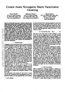
Figure 1: An example of the inter-type relationships and intra-type constraints. It is easy for us to judge whether two movies belong to the same class by their contents, titles, or actors, and it is also not hard to judge whether two persons belong to the same class by their ages, jobs, or hobbies. In this figure, the red lines stand for the must-links, and the blue dashed lines represent the cannot-links.

multiple type data points simultaneously. We can show that the traditional semi-supervised clustering methods [15] are just special cases of our framework when the data set is of only a single type. Finally the experimental results on several real world data sets are presented to show the effectiveness of our method. The rest of this paper is organized as follows. In Section 2 we introduce our Penalized Matrix Factorization (PMF) algorithm for constrained clustering. In Sections 3 and 4 we generalize our PMF based method to co-cluster dyadic and multi-type data sets with constraints. The experimental results are presented in Section 5, followed by the conclusions and discussions in Section 6. 2

Semi-Supervised Clustering Using Penalized Matrix Factorization In this section we introduce our penalized matrix factorization (PMF) for semi-supervised co-clustering. First let’s introduce some notations are frequently used in the rest of this paper.

The number of data points The number of clusters The i-th data point in Rd The data matrix of size d × n The cluster center of the c-th cluster The cluster center matrix The cluster indicator matrix The cluster indicator matrix of the i-th type data The constraint matrix The constraint matrix on the i-th type data The relationship matrix The relationship matrix between the i-th and j-th types of data

frequently used characters are summarized in Table 1. 2.2 Problem Formulation In this subsection we first review the basic problem of constrained clustering and introduce a novel algorithm called Penalized Matrix Factorization (PMF) to solve it. Given a data set X = {x1 , · · · , xn }, the goal of clustering is to partition the data set into C clusters π = {π1 , π2 , · · · , πC } according to some principles. For example, the classical kmeans algorithm achieves this goal by minimizing the following cost function X X Jkm = kxi − fc k2 , c

xi ∈πc

where fc is the center of cluster πc . If we define three matrices X = [x1 , x2 , · · · , xn ], F = [f1 , f2 , · · · , fC ] ∈ Rn×C , G ∈ Rn×C with its (i, j)-th entry Gij = gij , where ½ 1, if xi ∈ πj (2.1) gij = 0, otherwise then we can rewrite Jkm in the following matrix form (2.2)

°2 ° ° ° Jkm = °X − FGT °

F

where k · kF denotes the matrix Frobenius norm. Therefore, the goal of kmeans is just to solve G by minimizing Jkm , which can be carried out by matrix factorization techniques after some relaxations [12][11]. However, the organization of the data set in such 2.1 Notations Throughout the paper, we use bold a purely unsupervised way usually makes the results uppercase characters to denote matrices, bold lowercase unreliable since there is not any guidance from the data characters to denote vectors. The notations of some labels. Therefore, in recent years some researchers have

proposed semi-supervised clustering algorithms [4][15], which aim to cluster X into C clusters under the guidance of some prior knowledge on the data labels. One type of such prior knowledge assumes that only part (usually a limited part) of the training data are labeled [3], while the other type of prior knowledge is even weaker in that it only assumes the existence of some pairwise constraints indicating similarity or dissimilarity relationships between training examples [4]. In this paper, we consider the prior knowledge of the latter case. Typically, the knowledge that indicates the two points belong to the same class is referred to as mustlink constraints M, and the knowledge that indicates the two points belong to different classes is referred to as cannot-link constraints C. This type of information can be incorporated into traditional partitional clustering algorithms by adapting the objective function to include penalties for violated constraints. For instance, the Pairwise Constrained KMeans (PCKM) algorithm proposed in [4] modifies the standard sum of squared errors function in traditional kmeans to take into account both object-centroid distortions in a clustering π = {π1 , π2 , · · · , πC } and any associated constraint violations, i.e. X X X X θij + θ˜ij , J(π) = kxi − fc k2 +

we can rewrite J(π) as (2.4)

° °2 ° ° J(π) = °X − FGT ° + tr(GT ΘG) F

Note that for a general semi-supervised clustering algorithm, we are given X and Θ, and we want to solve F and G. By its definition, the elements in G can only take binary values, which makes the minimization of π unsolvable, therefore we propose to relax the constraint on G and solve the following optimization problem ° °2 ° ° minF,G J(π) = °X − FGT ° + tr(GT ΘG) F

(2.5)

s.t.

T

G > 0, G G = I

In our later derivations, we find it hard to solve the above optimization problem when both constraints being satisfied. Therefore, following the discussion in [12][19], we drop the orthogonal condition GT G = I and solve the following relaxed optimization problem ° °2 ° ° minF,G J(π) = °X − FGT ° + tr(GT ΘG) F

(2.6)

s.t.

G > 0.

Compared to the traditional (nonnegative) matrix factorization problem [12][10][18][11], we can find that the only difference in J(π) in the inclusion of the penalty xi ,xj ∈C xi ,xj ∈M c xi ∈πc s.t. li =lj s.t. li 6=lj term tr(GT ΘG), hence we call Eq.(2.6) a Penalized Matrix Factorization (PMF) problem, in the following where {θij > 0} represent the penalties for violating the we will introduce a simple iterative algorithm to solve must-link constraints, and {θ˜ij > 0} denote the penal- it. ties for violating the cannot-link constraints. Therefore, the goal of semi-supervised clustering is just to find an 2.3.1 The Algorithm The basic algorithm proceoptimal partition of X which can minimize J(π). dure for solving Eq.(2.6) is shown in Table 2. 2.3 Penalized Matrix Factorization for Constrained Clustering Following [15], we can change Table 2: Penalized Matrix Factorization for Constrained the penalties of violations in the constraints in M into Clustering the awards as X X X X Inputs: Data matrix X, Constraints matrix Θ. J(π) = kxi − fc k2 − θij + θ˜ij Outputs: F, G. xi ,xj ∈M xi ,xj ∈C c xi ∈πc 1. Initialize G using Kmeans as introduced in [11]; s.t. li =lj s.t. li =lj XX XX 2. Repeat the following steps until convergence: = gic kxi − fc k2 + gic gjc Θij (a). Fixing G, updating F by F = XG(GT G)−1 ; c xi c i,j (b). Fixing F,v updating G by ³ ´ u T + u (X F)ij +[G(FT F)− ]ij + Θ− G ij where ³ + ´ . Gij ←− Gij t T −  (X F)ij +[G(FT F)+ ]ij + Θ G ˜ ij (xi , xj ) ∈ C  θij , (2.3) Θij = −θij , (xi , xj ) ∈ M  0, otherwise

Defining matrix Θ ∈ Rn×n with its (i, j)-th entry 2.3.2 Correctness of the Algorithm Now let’s Θij = Θij , and applying the same trick as in Eq.(2.2), return to the optimization problem Eq.(2.6), where we

can expand the objective function J(π) as (2.7) J(π) = tr(XT X − 2FT XG + GFT FGT + GT ΘG)

which is equivalent to (−2XT F + 2GFT F + 2ΘG)ij G2ij = 0,

¤ Then the correctness of the algorithm in Table 2 is which is equivalent to Eq.(2.10). guaranteed by the following theorem. 2.3.3 Convergence of the Algorithm Now the Theorem 2.1. If the update rule of F and G in Table only remaining problem is to prove the algorithm in 2 converges, then the final solution satisfies the KKT Table 2 will finally converge. The same as in [17], we optimality condition. use the auxiliary function approach to achieve this goal. The auxiliary function is defined as follows. Proof. Following the standard theory of constrained optimization, we introduce the Lagrangian multipliers Definition 2.1. (Auxiliary Function) [17] A funcβ and construct the following Lagrangian function tion Z(G, G0 ) is called an auxiliary function of function L(G) if (2.8) L = J(π) − tr(βGT ) Then combining Eq.(2.8) and Eq.(2.7), we can derive that ∂L ∂F ∂L ∂G

T

= −2XG + 2FG G = −2XT F + 2GFT F + 2ΘG − β

Fixing G, letting

∂L ∂F

(2.9)

F = XG(GT G)−1

Fixing F, letting

∂L ∂G

= 0, we can get

= 0, we can get

β = −2XT F + 2GFT F + 2ΘG

Z(G, G0 ) > L(G), Z(G, G) = L(G) hold for any G, G0 . Let {G(t) } be the series of matrices achieved from the iterations of the algorithm in Table 2, where the superscript (t) represents the iteration number. Now let’s define G(t+1) = arg min Z(G, G(t) ), G

where Z(G, G0 ) is the auxiliary function for L(G) = J(π) in Eq.(2.7), then by its construction, we have

L(G(t) ) = Z(G(t) , G(t) ) > Z(G(t+1) , G(t) ) > L(G(t+1) ). the KKT complementary condition for the nonnegativity of G is Thus L(G(t) ) is monotonically decreasing. The thing T T remaining is to find an appropriate Z(G, G0 ) and its (2.10) (−2X F + 2GF F + 2ΘG)ij Gij = β ij Gij = 0 global minima. We have the following theorem. This is the fixed point equation that the solution must Theorem 2.2. Updating F and G using the rules satisfy at convergence. Therefore, let Eq.(2.9) and Eq.(2.11) will finally converge. Θ = Θ+ − Θ− Proof. Using the preliminary theorem in appendix II, FT F = (FT F)+ − (FT F)− and let B = XT F, A = FT F, we can get the auxiliary XT F = (XT F)+ − (XT F)− ˜ Thus let J(F, G) = J(π) in Eq.(2.7), function Z(G, G). where Θ+ , Θ− , (FT F)+ , (FT F)− , (XT F)+ , (XT F)− we can get that are all nonnegative. Then given an initial guess of G, J(F0 , G0 ) > J(F1 , G0 ) > J(F1 , G1 ) > · · · the successive update of G using (2.11) So J(F, G) is monotonically decreasing. Since J(F, G) v ¡ ¢ u T + is obviously bounded below, we prove the theorem. ¤ u (X F)ij + [G(FT F)− ]ij + Θ− G ij ¡ ¢ Gij ←− Gij t T − (X F)ij + [G(FT F)+ ]ij + Θ+ G ij 3 Penalized Matrix Tri-Factorization for Dyadic Constrained Co-Clustering will converge to a local minima of the problem. Since In the last section we have introduced a novel PMF at convergence, G(∞) = G(t+1) = G(t) = G, i.e. algorithm to solve the semi-supervised (constrained) (2.12) v ¡ − ¢ u T + clustering algorithm. One limitation of such algorithm u (X F)ij + [G(FT F)− ]ij + Θ G ij t is that it can only tackle the problem when there ¡ + ¢ Gij = Gij T + (XT F)− is only one single type of data objects, i.e. it can ij + [G(F F) ]ij + Θ G ij

only process the homogeneous data. However, as we stated in the introduction, many real world data sets are heterogeneous. In this section, we extend the PMF algorithm in Table 2 and propose a tri-PMF algorithm which can cope with the dyadic constrained co-clustering problem. 3.1 Problem Formulation In the typical setting of the dyadic co-clustering problem, there are two types of data objects, X1 and X2 with size n1 and n2 , and we are given a relationship matrix R12 ∈ Rn1 ×n2 , such that R12 (i, j) represents the relationship between i-th point in X1 and the j-th point in X2 . Usually R21 = RT12 . The goal of co-clustering is to cluster X1 and X2 simultaneously by making use of R12 . Many algorithms have been proposed to solve the dyadic co-clustering algorithm [2][6][8][9]. The authors in [11] proposed a novel algorithm called nonnegative matrix tri-factorization (tri-NMF) and showed that the solution of tri-NMF just corresponds to the relaxed solution of clustering the rows and columns of a relation matrix. More concretely, following the notations we introduced above, the nonnegative matrix tri-factorization aims to solve the following optimization problem (3.13)

min

G1 >0,G2 >0,S>0

kR12 − G1 SGT2 k2 ,

where G1 and G2 correspond to the cluster indicator matrices of X1 and X2 respectively. Note that the original NMF problem requires R12 to be nonnegative. In the co-clustering scenario, we can relax this constraint and solve the following optimization problem (3.14)

min

G1 >0,G2 >0

kR12 − G1 SGT2 k2 ,

which can be called semi-tri-NMF problem following [12]. As we stated in the introduction, we may also have some other information on X1 and X2 when we acquire them. In this paper, we consider those information are in the form of pairwise constraints on the same type of data objects, i.e., we have some must-link and cannotlink constraints on X1 and X2 respectively. Therefore the goal of constrained dyadic co-clustering is just to solve the following optimization problem (3.15)

min

G1 >0,G2 >0

kR12 − G1 SGT2 k2 + P (X1 ) + P (X2 ),

Eq.(2.4), we also assume here that P (X1 ) and P (X2 ) are of the following quadratic forms. (3.16) (3.17)

P (X1 ) = tr(GT1 Θ1 G1 ) P (X2 ) = tr(GT2 Θ2 G2 )

where Θ1 ∈ Rn1 ×n1 and Θ2 ∈ Rn2 ×n2 are the penalty matrices on X1 and X2 , such that Θ1 (i, j) and Θ2 (i, j) represent the penalty of violating the constraints between the i-th and j-th points in X1 and X2 as in Eq.(2.3). Then the goal of constrained dyadic coclustering is just to solve the following optimization problem (3.18) min

G1 >0,G2 >0

J = kR12 −G1 SGT2 k2 +tr(GT1 Θ1 G1 )+tr(GT2 Θ2 G2 )

which is just a problem to factorize R12 into three matrices G1 , S, G2 with some constraints and penalties, thus we call the problem Penalized Matrix TriFactorization (tri-PMF). 3.2.1 The Algorithm Table 3 provides a simple iterative algorithm to solve the optimization problem Eq.(3.15). Table 3: Penalized Matrix Tri-Factorization for Dyadic Constrained Co-Clustering Inputs: Relation matrix R12 , Constraints matrices Θ1 , Θ2 . Outputs: G1 , S, G2 . 1. Initialize G1 using Kmeans as introduced in [11]; 2. Initialize G2 using Kmeans as introduced in [11]; 3. Repeat the following steps until convergence: (a). Fixing G1 , G2 , updating S using S ←− (GT1 G1 )−1 GT1 R12 G2 (GT2 G2 )−1 ; (b). Fixing s S, G2 , updating G1 using −

G1ij ← G1ij

T T − (R12 G2 ST )+ ij +[G1 (S G2 G2 S) ]ij +(Θ1 G1 )ij T T + (R12 G2 ST )− ij +[G1 (S G2 G2 S) ]ij +(

Θ+ 1 G1 )ij

(c). Fixing s G1 , S, updating G2 using −

G2ij ← G2ij

+ T T − (RT 12 G1 S)ij +[G2 (SG1 G1 S ) ]ij +(Θ2 G2 )ij − T T + (RT 12 G1 S)ij +[G2 (SG1 G1 S ) ]ij +(

Θ+ 2 G2 )ij

3.2.2 Correctness of the Algorithm Returning to the problem Eq.(3.15), we can first expand J by

where P (X1 ) and P (X2 ) denote the penalties of the J = tr(RT12 R12 − 2GT2 RT12 G1 S + GT1 G1 SGT2 G2 ST ) constraint violations on X1 and X2 respectively. (3.19) +tr(GT1 Θ1 G1 ) + tr(GT2 Θ2 G2 ) 3.2 Constrained Dyadic Co-Clustering via Then the correctness of the algorithm in Table 3 is Penalized Matrix Tri-Factorization Similar to guaranteed by the following theorem.

.

;

Theorem 3.1. If the update rule of G1 , S and G2 in 3.2.3 Convergence of the Algorithm Now the Table 3 converges, then the final solution satisfies the only remaining thing is to prove the convergence of the KKT optimality condition. algorithm in Table 3. Similar to theorem 2.2, we have the following theorem. Proof. Similar to section 2.3, we introduce the Lagrangian multipliers β 1 and β 2 , and construct the fol- Theorem 3.2. Updating G1 , G2 , S using the rules in Table 3 will finally converge. lowing Lagrange function L = J − tr(β 1 GT1 ) − tr(β 2 GT2 )

(3.20) Then ∂L ∂S ∂L ∂G1 ∂L ∂G2

=

−2GT1 R12 G2 + 2G1 GT1 SGT2 G2

=

−2R12 G2 ST + 2G1 SGT2 G2 ST + 2Θ1 G1 − β 1

=

−2RT12 G1 S + 2G2 ST GT1 G1 S + 2Θ2 G2 − β 2

Fixing G1 , G2 , we can update S as (3.21)

S ←− (GT1 G1 )−1 GT1 R12 G2 (GT2 G2 )−1

Proof. Viewing J in Eq.(3.19) as a function of G1 , we can construct the auxiliary function based on the theorem in appendix II by setting B = R12 G2 ST , A = SGT2 G2 ST , G = G1 , Θ = Θ1 . Similarly, viewing J in Eq.(3.19) as a function of G2 , we can construct the auxiliary function based on the theorem in appendix II by setting B = RT12 G1 S, A = ST GT1 G1 S, G = G2 , Θ = Θ2 . Therefore J will be monotonically decreasing using the updating rules of G1 and G2 . Therefore, let J(G1 , S, G2 ) = J, then we have J(G01 , S0 , G02 ) > J(G01 , S1 , G02 ) > J(G11 , S1 , G02 ) > · · ·

So J(G1 , S, G2 ) is monotonically decreasing. Since Fixing S, G2 , we can get that the KKT complementary J(G1 , S, G2 ) is obviously bounded below, we prove the condition for the nonnegativity of G1 is theorem. ¤ (3.22) (−2R12 G2 ST +2G1 SGT2 G2 ST +2Θ1 G1 )ij G1ij = 0

Symmetric Penalized Matrix Tri-Factorization (tri-SPMF) for Multi-Type Constrained Co-Clustering G1ij ← In section 2 and section 3 we have introduced how v to solve the constrained clustering problem on uniu − T T − u (R12 G2 ST )+ + [G 1 (S G2 G2 S) ]ij + (Θ1 G1 )ij type or dyadic data sets using the penalized matrix ij G1ij t T GT G S)+ ] + (Θ+ G ) (R12 G2 ST )− + [G (S factorization based algorithm. A natural question would 1 2 ij 1 ij 2 1 ij be how to generalize those algorithm to the data sets It can be easily seen that using such a rule, at containing the data objects more than two types as convergence, G1ij satisfies many real world data sets have multiple types of data T T T 2 objects. In this section we introduce a novel algorithm (3.23) (−2R12 G2 S +2G1 SG2 G2 S +2Θ1 G1 )ij G1ij = 0 called symmetric penalized matrix tri-factorization (triwhich is equivalent to Eq.(3.22). SPMF) to solve such problem. Fixing S, G1 , we can get that the KKT complementary condition for the nonnegativity of G2 is 4.1 Problem Formulation We denote a K-type Then given an initial guess of G1 , we can successively update G1ij by

4

data set as X = {X1 , X2 , · · · , XK }, where Xi = {xi1 , xi2 , · · · , xini } represents the data set of type i. AsThen given an initial guess of G2 , we can successively suming we are also given a set of relation matrices update G2ij by {Rij ∈ Rni ×nj } between different types of data objects with Rji = RTij . Then the goal of co-clustering on X G2ij ← is just to cluster the data objects in X1 , X2 , · · · , XK siv u T multaneously [13][20][21]. − + T T − u (R12 G1 S)ij + [G2 (SG1 G1 S ) ]ij + (Θ2 G2 )ij In constrained multi-type co-clustering, we also G2ij t T + T T + (R12 G1 S)− ij + [G2 (SG1 G1 S ) ]ij + (Θ2 G2 )ij have some prior knowledge, i.e., must-link and cannotWe can also easily derive that at convergence, G2ij link constraints for each Xi (1 6 i 6 K). Therefore, we can construct a penalty matrix Θi for each Xi . The goal satisfies that is to cluster X1 , X2 , · · · , XK simultaneously by making use of Θ1 , Θ2 , · · · , ΘK . We denote the cluster indicator (3.25) (−2RT12 G1 S + 2G2 ST GT1 G1 S + 2Θ2 G2 )ij G22ij = 0 for Xi as Gi ∈ Rn+i ×Ci (Ci is the number of clusters in which is equivalent to Eq.(3.24). ¤ Xi ). Then a natural way to generalize the penalized

(3.24) (−2RT12 G1 S + 2G2 ST GT1 G1 S + 2Θ2 G2 )ij G2ij = 0

matrix tri-factorization for dyadic data to multi-type Proof. See appendix III. data is to solve the following optimization problem Combining Lemma 4.1 and Lemma 4.2 we can draw the (4.26) X X conclusion that it is equivalent to solve Eq.(4.27) and T T 2 min kRij − Gi Sij Gj k + tr(Gi Θi Gi ) F1 >0 Eq.(4.28). Since problem Eq.(4.28) is just to factorize a i F2 >0 00 (4.27) min kR12 − G1 S12 GT2 k2 G1 >0,G2 >0 where  n1 ×n1  1 ×nK can be equivalently solved by the following symmetric 0 Rn121 ×n2 · · · Rn1K matrix tri-factorization problem. 2 ×nK   Rn212 ×n1 0n2 ×n2 · · · Rn2K   R =   . . .. .. .. ..   (4.28) min kR − GSGT k2 , . . G>0 K ×n1 K ×n2 RnK1 RnK2 · · · 0nK ×nK  n1 ×C1  where G1 0n1 ×C2 · · · 0n1 ×CK · n ×n ¸  0n2 ×C1 Gn2 ×C2 · · · 0n2 ×CK  0 1 1 Rn121 ×n2 2   R = (4.29) n2 ×n1 G =   n2 ×n2 .. .. .. .. R21 0   . . . . · n1 ×C1 ¸ nK ×CK nK ×C1 G1 0n1 ×C2 0nK ×C2 · · · GK 0 (4.30) G =  C1 ×C1  0n2 ×C1 Gn2 2 ×C2 C1 ×C2 1 ×CK 0 S12 · · · SC 1K ¸ · C ×C 1 ×C2  SC2 ×C1 0C2 ×C2 · · · SC2 ×CK  0 1 1 SC 12 2K  21  (4.31) S = C2 ×C1 C2 ×C2 S =   .. .. .. S21 0 ..   . . . . where we use superscripts to denote the sizes of the matrices, and R21 = RT12 , S21 = ST12 . Proof. Following the definitions of G and S, we can derive that · ¸· ¸· T ¸ 0 S12 G1 0 G1 0 GSGT = 0 G2 ST12 0 0 GT2 · ¸· T ¸ 0 G1 S12 G1 0 = G2 ST12 0 0 GT2 · ¸ 0 G1 S12 GT2 = G2 ST12 GT1 0 Therefore kR − GSGT k2 °· ¸ · ° 0 R12 0 ° =° − RT12 0 G2 ST12 GT1

G1 S12 GT2 0

¸°2 ° ° °

= 2kR12 − G1 S12 GT2 k2 which proves the lemma.

 Θ

Lemma 4.2. The solutions to Eq.(4.27) using matrix tri-factorization and Eq.(4.28) using matrix trifactorization are the same.

CK ×C2 SK2

···

0CK ×CK 0n1 ×nK 0n2 ×nK .. .

Θn1 1 ×n1 0n2 ×n1 .. .

0n1 ×n2 Θn2 ×n2 .. .

··· ··· .. .

0nK ×n1

0nK ×n2

···

    

ΘnKK ×nK

in which Rji = RTij , Sji = STij . Proof. The proof of the theorem is a natural generalization of the proofs of lemma 4.1 and lemma 4.2. ¤ 4.2 The Algorithm Therefore, theorem 4.1 tells us that we can solve Eq.(4.26) by equivalently solving the symmetric penalized matrix tri-factorization (triSPMF) problem Eq.(4.32). More concretely, we have the following theorem. Theorem 4.2. Problem (4.32) can be solved via the following updating rule: (4.33)

¤

  =  

K ×C1 SC K1

(4.34)

S ← (GT G)−1 GT RG(GT G)−1

v ¡ ¢ u u (RGS)+ + [G(SGT GS)− ]ij + Θ− G ij ij ¡ + ¢ Gij ← Gij t T + (RGS)− ij + [G(SG GS) ]ij + Θ G ij

Table 4: Symmetric Penalized Matrix Tri-Factorization for Multi-Type Constrained Co-Clustering Inputs: Relation matrices {Rij }16i tr(ST ASB)

Sip

Proof. See theorem 6 in [11]. Appendix II: A Preliminary Theorem Theorem 6.1. Let (6.35) J(G) = tr(−2GT B + GAGT ) + tr(GT ΘG)

where A, Θ are symmetric, G is nonnegative. Then the following function à ! 5.2.2 Experimental Settings In our experiments, X Gij + 0 0 Z(G, G ) = −2 Bij Gij 1 + log 0 there are three data types: topics (X1 ), user IDs (X2 ) Gij ij and boards (X3 ). The topic-user matrix(R12 ) was 2 X constructed with the number of articles each user post G2ij + G0 ij X (G0 A+ + Θ+ G0 )ij G2ij + B− + in each topics with TF-IDF normalization [1]. The ij G0ij 2G0 2ij ij ij topic-board matrix (R13 ) was constructed such that à ! X if a topic belongs to a board, then the corresponding Gij Gik 0 0 − A− element of R13 is 1. R23 was constructed such that if jk Gij Gik 1 + log G0ij G0ik ijk the user had posted any articles on that board, then ! à X the corresponding element of R23 is set to 1. Finally G G ji ki 0 0 − Θ− jk Gji Gki 1 + log the elements of R23 were also normalized in a TFG0ji G0ki ijk IDF way. In our method, we randomly generate 500 constraints on X2 based on their registered profiles, 100 is an auxiliary function for J(G). Furthermore, it is a constraints on X1 based on the boards they belong to, convex function in G and its global minimum is v and 10 constraints on X3 based on their corresponding ¡ − ¢ u − u (B)+ fields. Besides our algorithm, the results of applying ij + [GA ]ij + Θ G ij t ¡ + ¢ Gij = Gij the Spectral Relational Clustering (SRC) method [21] (6.36) + (B)− ij + [GA ]ij + Θ G ij and Multiple Latent Semantic Analysis (MLSA) method [24] are also presented for comparison. The evaluation Proof. We rewritten Eq.(2.7) as metric is also the F score computed based on the J(G) = tr(−2GT B+ + 2GT B− + GA+ GT − GA− GT ) clustering results on topics, the ground truth of which +tr(GT Θ+ G − GT Θ− G) is set to be the classes corresponding to the field name they belong to. by ignoring tr(XT X). By applying the proposition in 5.2.3 Experimental Results The experimental results are shown in Table 9, in which the value of d represents the different number of clusters we set. From the table we can clearly see the effectiveness of our algorithm (note that the F scores of our tri-SPMF algorithm are the values averaged over 50 independent runs).

appendix I, we have tr(GT Θ+ G) 6

X (Θ+ G0 )ij G2ij ij

tr(GA+ GT ) 6

G0ij

X (G0 A+ )ij G2ij ij

G0ij

Data Sets 1 1 1 2 2 2 3 3 3

Table 9: Algorithm MLSA SRC Tri-SPMF MLSA SRC Tri-SPMF MLSA SRC Tri-SPMF

The F measure of d=3 d=4 0.7019 0.7079 0.7281 0.6878 0.7948 0.8011 0.7651 0.7429 0.7627 0.7226 0.8007 0.7984 0.6689 0.6511 0.7556 0.7666 0.8095 0.8034

three algorithms on d=5 d=6 0.7549 0.7541 0.6183 0.6183 0.8021 0.7993 0.7581 0.7309 0.7280 0.6965 0.7938 0.7896 0.6987 0.7301 0.7472 0.7125 0.7993 0.7874

Moreover, by the inequality

the three d=7 0.7081 0.6103 0.7754 0.7284 0.6972 0.7810 0.7236 0.6758 0.7703

Φij

We have −

tr(G B ) =

X

B− ij Gij

d = 10 0.7066 0.4268 0.7590 0.6856 0.5949 0.7754 0.6953 0.6456 0.7492

is a diagonal matrix with positive diagonal elements

a 6 (a2 + b2 )/2b, f or ∀ a, b > 0

T

data sets d=8 d=9 0.7031 0.6990 0.6029 0.4783 0.7732 0.7653 0.7063 0.6806 0.6620 0.6570 0.7763 0.7801 0.7045 0.7197 0.6887 0.6636 0.7722 0.7665

6

X

ij

=

2(B+ + G0 A− + ΘG0 )ij G0ij G2ij

2

B− ij

G2ij + G0 ij

ij

+

(6.38)

2G0 2ij

2(B− + G0 A+ + ΘG0 )ij G0ij

To obtain the lower bounds for the remaining terms, we Thus Z(G, G0 ) is a convex function of G. Therefore, we use the inequality that z > 1 + log z, which holds for can obtain the global minimum of Z(G, G0 ) by setting ∂Z(G, G0 )/∂Gij = 0 and solving for G, from which we any z > 0, then can get Eq.(6.36). ¤ Gij Gij > 1 + log G0ij G0ij Appendix III: Proof of Lemma 4.2 Gij Gik Gij Gik Proof. It can be easily inferred that (from the derivation > 1 + log 0 0 G0ij G0ik Gij Gik in section 3) the updating rules for solving Eq.(4.27) are Then tr(GT B+ ) >

X

à 0 B+ ij Gij

1 + log

ij −

T

tr(G Θ G) >

X

à 0 0 Θ− jk Gji Gki

ijk −

T

tr(GA G ) >

X

à 0 0 A− jk Gij Gik

ijk

Gij G0ij

!

Gji Gki 1 + log 0 0 Gji Gki

Gij Gik 1 + log 0 0 Gij Gik

!

G0ij 2(G0 A+ )ij Gij ∂Z(G, G0 ) Gij + = −2B+ + 2B− ij ij 0 ∂Gij Gij Gij G0ij −

2(G0 A− )ij G0ij 2(Θ G0 )ij G0ij 2(Θ+ G0 )ij Gij − + 0 Gij Gij Gij

and the Hessian matrix for Z(G, G0 ) (6.37)

∂Z(G, G0 ) = δik δjl Φij ∂Gij ∂Gkl

←

G1ij

←

G2ij

←

!

By summing over all the bounds, we can get Z(G, G0 ), which clearly satisfies (1) Z(G, G0 ) > J(G); (2) Z(G, G) = J(G). To find the minimum of Z(G, G0 ), we take

−

S12

(GT1 G1 )−1 GT1 R12 G2 (GT2 G2 )−1 v u T T − u (R12 G2 ST12 )+ ij + [G1 (S12 G2 G2 S12 ) ]ij G1ij t T − T T (R12 G2 S12 )ij + [G1 (S12 G2 G2 S12 )+ ]ij v u T T T − u (R12 G1 S12 )+ ij + [G2 (S12 G1 G1 S12 ) ]ij G2ij t T − T (R12 G1 S12 )ij + [G2 (S12 G1 G1 ST12 )+ ]ij

Using the similar approach, we can derive the updating rules for solving Eq.(4.28) are S ← (GT G)−1 GT RG(GT G)−1 v u T − u (RGS)+ ij + [G(SG GS) ]ij Gij ← Gij t − (RGS)ij + [G(SGT GS)+ ]ij Due to the special block-diagonal form of R, G and S (see Eq.(4.29)-Eq.(4.31)), we can get that · T ¸· ¸ · T ¸ G1 0 G1 0 G1 G1 0 T G G= = 0 G2 0 GT2 0 GT2 G2 · GT RF =

0 GT2 RT12 G1

GT1 R12 G2 0

¸

Then · (GT G)−1 GT RG(GT G)−1 =

0 ˜T S

˜ S 0

¸

˜ = (GT G1 )−1 GT R12 G2 (GT G2 )−1 , which where S 1 1 2 shows the equivalence between the updating rules of S and S12 . Moreover, it also suggests that when updating S in solving the symmetric semi-tri-NMF problem Eq.(4.28), we only need to update the corresponding S12 part in S (see the definition of S in Eq.(4.31)). Similarly, we can get that ¸ · 0 R12 G2 ST12 RGS = 0 RT12 G1 S12 · T

SF FS =

S12 GT2 G2 ST12 0

0 ST12 GT1 G1 S12

¸

Bringing these two equations back to the updating rule of Gij , we can observe that the rules for updating the corresponding part G1 , G2 in G (see the definition of G in Eq.(4.30) are equivalent to the updating rules of G1 and G2 in solving Eq.(4.27). Therefore the solutions to Eq.(4.28) are equivalent to the solutions to Eq.(4.27).¤

References [1] R. Baeza- Yates and B. Ribeiro-Neto. Modern Information Retrieval. Addison-Wesley, 1999. [2] A. Banerjee, I. S. Dhillon, J. Ghosh, S. Merugu, and D. S. Modha. A Generalized Maximum Entropy Approach to Bregman Co-Clustering and Matrix Approximations. In Proc. of SIGKDD, 509-514, 2004. [3] S. Basu, A. Banerjee, and R. J. Mooney. Semisupervised Clustering by Seeding. Proc. of ICML, 2002. [4] S. Basu, M. Bilenko, and R. J. Mooney. A Probabilistic Framework for Semi-Supervised Clustering. In Proc. of SIGKDD, 59-68, 2004. [5] M. Bilenko, S. Basu, and R. J. Mooney. Integrating constraints and metric learning in semi-supervised clustering. In Proc. of ICML, 2004. [6] H. Cho, I. S. Dhillon, Y. Guan, and S. Sra. Minimum Sum-Squared Residue Co-clustering of Gene Expression Data. In Proc. of the SIAM SDM, 114-125, 2004. [7] F. R. K. Chung. Spectral Graph Theory. American Mathematical Society. 1997. [8] I. S. Dhillon. Co-Clustering Documents and Words Using Bipartite Spectral Graph Partitioning. Proc. of SIGKDD, 269-274. 2001. [9] I. S. Dhillon, S. Mallela, and D. S. Modha. InformationTheoretic Co-clustering. Proc. of SIGKDD, 2003. [10] C. Ding, X. He, and H. D. Simon. On the Equivalence of Nonnegative Matrix Factorization and Spectral Clustering. Proc. SIAM SDM, pp:606-610. 2005.

[11] C. Ding, T. Li, W. Peng, and H. Park. Orthogonal Nonnegative Matrix Tri-factorizations for Clustering. In Proc. of SIGKDD, 126-135. 2006. [12] C. Ding, T. Li, and M. I. Jordan. Convex and SemiNonnegative Matrix Factorizations. LBNL Tech Report 60428. 2006. [13] B. Gao, T.-Y. Liu, X. Zheng, Q.-S. Cheng, and W.Y. Ma, Consistent Bipartite Graph Co-Partitioning for Star-Structured High-Order Heterogeneous Data CoClustering. In Proc. of SIGKDD, pp. 41-50, 2005. [14] Z. Kou, and C. Zhang. Reply Networks on a Bulletin Board System. Phys Rev E, 2003, 67(3-2): 036117. [15] B. Kulis, S. Basu, I. Dhillon, R. J. Mooney. SemiSupervised Graph Clustering: A Kernel Approach. In Proc. of ICML, 457-464, 2005. [16] B. Larsen, C. Aone. Fast and Effective Text Mining Using Linear-time Document Clustering. In Proc. SIGKDD, pp 16-22. [17] D. D. Lee and H. S. Seung. Algorithms for Nonnegative Matrix Factorization. NIPS 13, 556-562, 2001. [18] T. Li and C. Ding. Relationships Among Various Nonnegative Matrix Factorization Methods for Clustering. Proc. of ICDM. pp.362-371. 2006. [19] T. Li, C. Ding and M. I. Jordan. Solving Consensus and Semi-supervised Clustering Problems Using Nonnegative Matrix Factorization. In Proc. of ICDM. 2007. [20] B. Long, X. Wu, Z. (Mark) Zhang, and P. S. Yu. Unsupervised Learning on K-partite Graphs, In Proc. of SIGKDD, 317-326, 2006. [21] B. Long, Z. (Mark) Zhang, X. Wu, and P. S. Yu, Spectral Clustering for Multi-Type Relational Data, In Proc. of ICML, 2006. [22] K. Wagstaff, C. Cardie, S. Rogers, and S. Schroedl. Constrained k-means clustering with background knowledge. In Proc. of ICML, 2001. [23] H. Zha, C. Ding, M. Gu, X. He, H. Simon. Spectral Relaxation for K-means Clustering, NIPS 14. 2001. [24] X. Wang, J. Sun, Z. Chen, and C. Zhai. Latent semantic analysis for multiple-type interrelated data objects. SIGIR, 2006.