Semi-supervised Multi-task Learning of Structured Prediction Models for Web Information Extraction Paramveer S. Dhillon
S Sundararajan
[email protected]
[email protected]
University of Pennsylvania Philadelphia PA, U.S.A
Yahoo! Labs Bangalore, India
S Sathiya Keerthi
Yahoo! Labs Santa Clara, CA, U.S.A
[email protected]
ABSTRACT
1.
Extracting information from web pages is an important problem; it has several applications such as providing improved search results and construction of databases to serve user queries. In this paper we propose a novel structured prediction method to address two important aspects of the extraction problem: (1) labeled data is available only for a small number of sites and (2) a machine learned global model does not generalize adequately well across many websites. For this purpose, we propose a weight space based graph regularization method. This method has several advantages. First, it can use unlabeled data to address the limited labeled data problem and falls in the class of graph regularization based semi-supervised learning approaches. Second, to address the generalization inadequacy of a global model, this method builds a local model for each website. Viewing the problem of building a local model for each website as a task, we learn the models for a collection of sites jointly; thus our method can also be seen as a graph regularization based multi-task learning approach. Learning the models jointly with the proposed method is very useful in two ways: (1) learning a local model for a website can be effectively influenced by labeled and unlabeled data from other websites; and (2) even for a website with only unlabeled examples it is possible to learn a decent local model. We demonstrate the efficacy of our method on several real-life data; experimental results show that significant performance improvement can be obtained by combining semi-supervised and multi-task learning in a single framework.
Extracting information from web pages is an important problem. It has several web applications such as providing improved search results, serving user queries related to reviews, pricing information of products, etc., using databases constructed from information extraction. We consider the problem of domain-centric extraction where a schema corresponding to a domain of interest is given. The goal is to extract attributes specified by the schema from a collection of pages. Examples of a domain include Books, Restaurant, Publications etc. The schema for the Books domain will have attributes such as Title, Author, Publisher and Price. The pages for this domain are obtained from a collection of websites like www.amazon.com, www.booksamillion.com, etc. Similarly, a schema for the Publications domain will have attributes such as Author, Title, Conference, Pages etc., and these can be extracted from home pages of faculty members of different universities. In all these examples, the attributes of interest are often organized either as records in a list page or as a single record in a detail page. Each record is a set of attribute values of one entity, e.g., a Book or a Publication. Unsupervised methods [11, 39, 3, 25] are very successful in extracting records from list pages using structural patterns present in one or more web pages. In the case of a detail page, the informative region of the web page plays the role of a record and it can be obtained using methods such as the ones proposed in [38]. Therefore, throughout this paper we will assume that records are given and focus on the finer and challenging problem of extracting attributes from records. It is worth noting that the unsupervised methods mentioned above are inadequate for solving this attribute extraction problem. The problem is challenging due to the following reasons: (1) there are wide variations in presentation style of information across the websites. For example, attribute ordering, font size, font type (e.g., italic, capital), html tag structures, etc., are often different, (2) the number of websites is large, and (3) some of the attributes are optional (may not be present in all the records) and some of the attributes are missing (in all the records from a website). These reasons also make it hard to build a global model that generalizes well across the websites. Other challenges arise from the approach taken to address the extraction problem. For example, the wrapper induction [19, 27] method requires supervision; it utilizes labeled data to learn extraction rules on the HTML tag structure of pages. The need to have labeled data for each website and the presence of noisy structures within a website makes this method impractical for scaling to a large number of websites.
Categories and Subject Descriptors: H.3.m [Information Storage and Retrieval] Miscellaneous - Information Extraction, Web General Terms: Algorithms, Experimentation Keywords: Information Extraction, Semi-supervised learning, Multi-task learning, Structured Predictions
Permission to make digital or hard copies of all or part of this work for personal or classroom use is granted without fee provided that copies are not made or distributed for profit or commercial advantage and that copies bear this notice and the full citation on the first page. To copy otherwise, to republish, to post on servers or to redistribute to lists, requires prior specific permission and/or a fee. CIKM’11, October 24–28, 2011, Glasgow, Scotland, UK. Copyright 2011 ACM 978-1-4503-0717-8/11/10 ...$10.00.
INTRODUCTION
In recent years there has been a significant amount of research work done in building machine learned models for web information extraction. [5, 1, 29, 30, 41] apply sequential models like Hidden Markov Models (HMM), Conditional Random Fields (CRF) and Markov Logic Networks (MLN) to segment instances such as citations and addresses. All these methods focus on building a global model. Global models do not generalize well across websites whenever there are wide variations in structure and formatting across the websites (as frequently observed in domain-centric extraction problem). We demonstrate this issue using CRF models on the attribute extraction problem from records. This issue is expected to arise even when sophisticated models like hierarchical CRFs (HCRF) [41] and MLNs [30] are used. The key reason for this is that important features (e.g., attribute ordering, font type) that are discriminative within a site tend to become less effective whenever these features vary widely in the training examples from different websites. This problem can be alleviated by building local models where these discriminative features can be effectively made use of. Note that although we use a simple CRF model in our attribute extraction problem to demonstrate the usefulness of local models, our approach is quite generic and can be extended with HCRFs and MLNs. Therefore, our intention in this paper is not to demonstrate superiority over any of the existing information extraction methods using HCRF or MLN models; hence, we do not make any such comparisons. Our focus is on demonstrating the usefulness of building machinelearned local models and how these models can be effectively learned jointly when the labeled examples are scarcely available. Building machine-learned models in supervised and semisupervised settings require labeled data. In our problem context, getting labeled data from each website is extremely difficult as the number of websites is large. Furthermore, it is expensive to get a large amount of labeled data even for a few websites, particularly for structured data (such as a sequence or a tree) where the number of nodes and attributes is large. The aim of the paper is to address two important aspects of the domain-centric extraction problem: (1) limited labeled data is available only for a small number of websites but plenty of unlabeled data is available from all the websites in a collection, and (2) a machine-learned global model does not generalize adequately well across many websites. Our approach is based on connecting examples from different websites through a graph and learning local models for the websites jointly via graph regularization (Section 4). It exploits the fact that although there are variations in the presentation styles across the websites, there is useful common information that exists across the websites. For example, attributes such as Author, Title, Conference, Pages have (similar) content features that are common across the websites; our approach makes good use of such information.
1.1 Our Contributions We propose a weight space based graph regularization method. Our method has several advantages. First, it can use unlabeled data to address the limited labeled data problem and falls in the class of graph regularization based semisupervised learning (SSL) approaches. In this aspect, our work is related to [20, 2]. But, our formulation is much simpler and a lot easier to implement with publicly available
software packages for structured predictions; unlike [20, 2] we directly work in the weight space formulation instead of the dual formulation. Next, to address the generalization inadequacy of a global model, we propose to build a local model for each website. Furthermore, we suggest to learn the local models jointly to address the limited labeled data aspect; again, the weight space based graph regularization method can be used for joint learning. Viewing the problem of building a local model for each website as a task, our method can also be seen as a graph regularization based multi-task learning (MTL) approach. Learning the models jointly via the proposed method is useful in two ways: (1) learning a local model for a website can be effectively influenced by labeled and unlabeled data from other websites to get improved performance; and (2) even for a website with only unlabeled examples it is possible to learn a decent local model for it (which is not possible even for wrapper learning approaches). Thus, our method addresses the limited labeled data aspect via a unified framework for semi-supervised and multi-task learning. From a multi-task learning viewpoint, our work is related to [13]. However, our formulation goes beyond binary/multi-class problems, applies to structured prediction models, and is suitable for web information extraction. We are not aware of any work on multi-task learning that addresses the problem of learning local structured prediction models for totally unlabeled websites. We conduct experiments on several real world datasets constructed from web pages of domains such as Books, CSFaculty, Seminars and MLConfs. The experimental results demonstrate the effectiveness of the proposed method for semi-supervised, multi-task and semi-supervised multitask (combined semi-supervised and multi-task) learning scenarios. The results also show that the performance of local models built for totally unlabeled websites is better than that of the global model.
2.
PROBLEM FORMULATION
Consider the problem of extracting attributes from a given set of records. Let x and y denote the input and output representation of a record. We choose a suitable tokenization and view each record as a sequence of nodes; x is a sequence of feature vectors that are functions of the textual content and/or certain structural properties of these nodes; y is a sequence of labels assigned to these nodes where each label belongs to a label space Y. For example, the label space of a publication record could be {Author, Title, Date, Conference, Pages, Others}. We use the terms record, example and sequence interchangeably in this paper. Data: Assume that we have a set of labeled and unlabeled examples. These examples come from a collection of websites: S = {S1 , S2 , . . . , SM }. Let SL denote the set of websites which contain at least one labeled example. Websites in SL can also have unlabeled examples. Let SU denote the set of websites in which we have only unlabeled examples; |SU | and |SL | denote the cardinalities of SU and (m) (m) SL . Let (xi , yi ) denote the i-th example in Sm and (m) (m) let Tm = {(xi , yi ) : i = 1, . . . nm } denote the training set in Sm . Let Lm and Um denote the set of indices of the labeled and unlabeled sequences from Sm . Thus, a label (m) yi is available only if Sm ∈ SL and i ∈ Lm . Finally, let TM = ∪ M m=1 Tm where M = {1, . . . , M }.
Problem Formulation (Local Models): We are interested in building a local probabilistic model p(y|x; Wm ) for each website Sm to extract the attributes from the sequences. Wm denotes the local model weight vector of Sm . Thus, given a set of labeled and unlabeled examples from S, the goal is to learn the local model weights W = {Wm : m = 1, 2, . . . , M }. When we have only labeled examples, we can build the local models by optimizing the objective function L(TM , W) defined as: λ X 1 X (m) (m) ||Wm ||2 − log p(yi |xi ; Wm ) (1) 2 m:S ∈S |Lm | i∈L m
m
L
where λ > 0 is a regularization constant. Note that in the absence of connections between the learning tasks of the websites, (1) becomes separable. For such a case, the local model for each website is built separately using only the labeled examples from that website. We will refer to the models built in this scenario simply as the Local models. Problem Formulation (Global Model): Traditional extraction models learn a global weight vector W that is same for all websites. When we have only labeled examples, the global model is built by optimizing the objective function L(TM , W) defined as: X |SL |λ 1 X (m) (m) ||W||2 − log p(yi |xi ; W). (2) 2 |L m| m:S ∈S i∈L m
L
m
We will refer to the model thus built as the Global model. Recall the two main goals of this paper: (1) to address the limited labeled data problem and (2) to overcome the generalization inadequacy of a global model. We address these problems through a graph regularization based semisupervised multi-task learning method. The use of unlabeled examples results in semi-supervised learning. The problem of building a local model for each website can be viewed as one task; and, learning the models jointly results in multitask learning. Now, the objective functions (1) and (2) are not adequate for semi-supervised learning (SSL) as there are no terms that involve unlabeled examples. It is also not adequate for multi-task learning (MTL) because there are no terms that connect the multiple tasks. Thus, to facilitate SSL and MTL we propose to add a weight space based graph regularization term G(W) to the objective functions (1) and (2). Before we present our approach, we give details of the probabilistic model for sequences that we use in this paper.
3. CRF MODEL We now make precise, the probabilistic model p(y|x; W) for sequences used in the previous section. Given a record, we pose the problem of extracting attributes as a sequence labeling problem. For this purpose, we use the conditional random field (CRF) model [21]. CRF is a Markov random field that defines a conditional distribution of the labels y of a sequence conditionedQon the input x in the following form: p(y|x; W) = Z1x c∈C ψ(xc , yc ) where: W denotes the model weights; C is the set of cliques present in the sequence; yc denotes the components of y present in a clique c; ψ(·) is a potential function that takes nonnegative values; P Q and, Zx is the partition function defined The potential functions are as Zx = y c∈C ψ(xc , yc ). P expressed as: ψ(xc , yc ) = exp( k wk fk (xc , yc )) where the
fk (xc , yc )s are feature functions. Then, we have: p(y|x; W) =
`X X ´ 1 exp wk fk (xc , yc ) . Zx c∈C
(3)
k
In linear chain sequence labeling problems [21], common feature functions are represented as fk (xc , yc ) where c is either a node clique c with yc ∈ Y or an edge clique c connecting two adjacent nodes in a sequence, with yc ∈ Y 2 . Thus, we have two types of feature functions, namely, node and edge feature functions. In general the individual feature functions take real values; in many cases they are boolean. For example, a node feature function fk (xc , yc ) = I(xc ∈ AddressDictionary) ∧ (yc = Address) is TRUE when the textual content of xc is in the address dictionary and assigned label Address. Here, I(·) is the indicator function taking value 1 when the argument is TRUE and 0 otherwise. In supervised learning, the CRF model weights W are learned using a set of labeled training examples, T = {(xi , yi ) : i = 1, . . . , n} by minimizing a regularized P negative log likelihood function: L(T, W) = λ2 ||W||2 − n1 n i=1 log p(yi |xi ; W). P Thus, the function in (1) is L(TM , W) = M m=1 L(Tm , Wm ). The objective functions (such as L(T, W)) considered in this paper do not have closed form solutions to their minimizers; so, the optimal solutions are obtained by using optimization techniques like L-BFGS. Finally, using the learned weights, the optimal labeling of a new sequence (referred as inference) ˆ = argmaxy p(y|x; W), and is obtained using is defined as: y the Viterbi algorithm.
4.
OUR APPROACH
In this section we present our weight space based graph regularization method. This method can be used in one of the following three modes: (1) semi-supervised learning using labeled and unlabeled examples; (2) multi-task learning of local models; and (3) combined semi-supervised and multi-task learning of local models. The third combined setting is especially powerful since local models can be learned even for websites with only unlabeled examples. Our approach is to construct a graph that connects sequences from same or different websites. The basic idea is to make use of common information that exist across the sequences in influencing the node labels of the sequences. That is, if two nodes belonging to two different records have nearly the same features firing then these nodes are highly likely to have the same label. We illustrate this idea through some examples. Consider two publication records, one each from two different conference websites. Such records consist of nodes with labels such as Author, Title, Affiliation. For example, suppose we have node j and the node features are: I(FirstLetterCapital(xj )), I(xj ∈ AuthorDictionary), I(xj ∈ TechTermDictionary) and I(ContainsPunctuation(xj+1 )). Let us say node j has label Author. The contents of this node may be such that the three features other than I(xj ∈ TechTermDictionary) fire. Suppose there is another node j 0 with content such that the same set of features fire. It is very likely that the node j 0 also has the label Author. For some other node j 00 let us say the feature I(xj ∈ AuthorDictionary) also does not fire. It is likely that j 00 also has Author as the label, but to a lesser extent than j 0 . Thus, it is reasonable to capture our belief that two nodes have the same label by
using a similarity score computed from their feature vectors (e.g., the number of features that are commonly fired)1 . We can extend this idea to connect an edge (i.e., a pair of adjacent nodes) in one record to an edge in another record. In this case, for computing similarity we concatenate the feature vectors of the two nodes that constitute the edge. If two edges have similar concatenated feature vectors then it is very likely that both have the same label pairs. Connecting such edges (i.e., putting pressure to make them have the same label pairs) is certainly very useful for improving a local model since the same label ordering is expected in all records of one website. Even in the case of edge connections going across websites with different attribute ordering, the edge connections are useful in handling self transitions such as (Title,Title) and (Author,Author). Which features should we use for determining similarity? Clearly, using global features that are useful both within and across websites is a good idea. Within a local model, it is also helpful to use local features. For example, XPath features (i.e., html tag structure with some DOM node properties) are very useful for structured pages, where DOM nodes with the same XPath are expected to have the same label. Similarly, we may expect an attribute to have the same formatting properties, e.g., FontSize, FontType (i.e., bold, italic), etc. Due to the local nature of such features, we can connect nodes using these features only within each website and not across websites. To encode our expectation that similar nodes (or edges) have same label (label pair), we enforce their class marginal probabilities to be close, through regularization. Note that marginal probability computation takes the entire sequence into account. Below, we formalize the above idea, and facilitate SSL and MTL by adding a graph regularization term G(W) to the objective functions (1) and (2). Graph Regularization: The graph regularization term is a function defined on a graph G. The graph G consists of a set of vertices (V) and connections (O). To avoid confusion, we use the terminologies (node,edge) for the CRF cliques in the input sequences, and (vertex,connection) for the graph G. Each vertex has a score vector and each connection has a weight. A connection weight is a similarity score computed using features of the vertices involved in the connection. The vertices correspond to the nodes and edges of the sequences. Then, the graph regularization term is defined using the connection weights and vertex scores. As we show below, the vertex scores are dependent on the model weights. Thus, the method derives the name weight space based graph regularization. The basic idea is to regularize the model weights by constraining the scores of a pair of vertices to be close when their connection weight is large. Before we define the graph regularization term, we first explain how: (1) vertices are formed and connected, (2) connection weights are computed and (3) vertex scores are assigned. Vertices and Connecting Sequences: The role of G is to connect the sequences using some similarity measure. From section 3, we know that a sequence is characterized by a set of node and edge cliques, where an edge connects two ad1 Relational information has been used for collective classification of web documents; see for example, [23, 17, 33]. However, our work is different as we work with structured prediction models in the information extraction context; furthermore, we build local models.
jacent nodes. We connect two sequences by connecting the cliques of the sequences. Thus, each clique forms a vertex in G. With this definition, a vertex v is indexed by a 3-tuple (m, i, c) where c is a clique in the i-th sequence from the mth website. Let N and E denote the sets of node and edge cliques in the collection of sequences. We have V = N ∪ E and |V| = |N | + |E|. Two cliques (vertices) are connected only if they are of the same type. In other words, a node (edge) clique is connected only to other node (edge) cliques. Graph Structure: G is constructed by connecting cliques of labeled and unlabeled sequences obeying the above type constraint. Thus, G has two separate components which we refer to as node graph GN and edge graph GE . Connection Weights Computation: We now give details on finding the connection weight φv,v0 for each connection (v, v 0 ) ∈ G. From Section 3 we know that the feature functions fk (xc , yc ) are dependent on different features illustrated above. There will be many such features for a clique c and we collect these features into a feature vector Fv . Note that for an edge clique we collect feature vectors of both the nodes into a single feature vector. Using feature vectors of the vertices in a connection, we set the connection weight as: φv,v0 = D(Fv , Fv0 ) ≥ 0, a similarity score between the feature vectors. An example of a similarity score is the inner product of the two feature vectors. Thus, when the feature vectors of the two vertices (v, v 0 ) are similar, φv,v0 → 1 and when they are dissimilar φv,v0 → 0. The connection weights of GN and GE can be collected into two separate matrices, ΦN and ΦE . Note that ΦN is of size |N | × |N | and ΦE is of size |E| × |E|. When the number of examples (particularly, with the unlabeled examples) is large these matrices can be huge. Therefore, it is useful from storage and computational viewpoints to construct sparse matrices by connecting each vertex to only its k nearest neighbors. In our information extraction application, the number of features is small; therefore, defining a distance metric and finding nearest neighbors are not difficult. Vertex Scores Computation: To encode our expectation that vertices having similar feature vectors have the same label, we assign the class marginal probability distribution as the score vector for each vertex. Note that for each clique c, the marginal probability distribution is defined over all possible label assignments of yc . Thus, the score vector is of size |Y| for a node clique, and is of size |Y|2 for an edge clique. Let us call this score vector of a vertex v as (gv ). For notational simplicity we have suppressed the dependence of gv on the weights and the nodes associated with the clique. Graph Regularization Term G(W): Given G, vertex scores, gv , ∀v ∈ V and connection weights, φv,v0 , ∀(v, v 0 ) ∈ O, we define G(W) as: µN X µE X φv,v0 D(gv , gv0 ) + φv,v0 D(gv , gv0 ) (4) ZN ZE 0 0 v,v ∈N
v,v ∈E
where µN and µE are regularization constants; D(·) is a divergence measure such as Kullback-Leibler or squared error loss; ZN and ZE are graph normalization2 terms defined 2 Other graph normalization schemes such as normalizing the connection weights by the degree of a vertex are also posφ 0 sible. For example, use φ˜v,v0 = P 0 v,v φ 0 , ∀v ∈ GN and v ∈GN
v,v
P P 0 0 as ZN = v,v 0 ∈E φv,v . Other v,v 0 ∈N φv,v and ZE = graph normalization schemes can also be used. Thus, the graph regularization term connects the sequences by connecting their cliques. The first and second terms represent contributions from the node graph GN and the edge graph GE respectively. The model weights are regularized by constraining the scores of the cliques to be close whenever the similarity score between the cliques is large. With the introduction of (4) the objective functions associated with the Local and Global models in (1) and (2) get P modified to L(TM , W) + λ2 m:Sm ∈SU ||Wm ||2 + G(W) and
L(TM , W) + |SU2 |λ ||W||2 + G(W) respectively. Note that weight regularization corresponding to SU is also added. The complexity of function and gradient computations of gv is O(|F |V ) where |F | and V are the feature size and sequence length respectively; this causes the optimization of the above mentioned objective functions to be expensive for large datasets. Therefore, to reduce the computational cost, we use an alternate score vector. From (3), we see that thePscore of a sequence (x, y) can be defined as: H(x, y) = c∈C hc (xc , yc ; W) where hc (xc , yc ; W) = P k wk fk (xc , yc ) is the score contribution from clique c and is dependent on yc . Thus, for each clique c, we compute gv comprising of the scores corresponding to all possible label assignments of yc . Note that gv is linear in the model weights; therefore, the function and gradient computations are cheap. There is an additional advantage associated with using the alternate score vector. Since gv is linear in the model weights and φv,v0 ≥ 0, ∀v, v 0 ∈ V, each of the sub-terms in (4) is quadratic in the model weights, and is convex. Note that (2) and (1) are also convex. Therefore, adding (4) to (2) or (1) results in a convex optimization problem with a unique solution. This solution is easily and dependably obtained by using optimization techniques like L-BFGS. The alternate score is not just cheaper; our experimental results (see the next section) show that very good generalization performance is achieved with it. Finally, with learned W, the Viterbi algorithm is used to make predictions.
Learning Scenarios: Let us revisit the three modes of using G mentioned at the beginning of this section. We make use of G for two purposes. It is used to connect the examples (labeled and unlabeled), and it is also used to connect multiple tasks by connecting the examples of two different tasks. We show below how different learning scenarios can be created by setting up the graph in different ways. In each scenario the solution is obtained by using optimization techniques like L-BFGS (as in supervised learning). (1) Semi-supervised Learning: In the Global model scenario, G connects the examples (labeled and unlabeled) across all the websites (S). In the Local models scenario, G connects the examples (labeled and unlabeled) only within each website. In this scenario, the examples from SU are not used, and the local models can be learned independently as there are no connections between the examples from different sites. In these scenarios, the unlabeled examples are also used to learn the models. We refer the models built in these scenarios as SSL-Global and SSL-Local model(s) respectively. (2) Multi-task Learning: This is applicable only in the set ZN = |N1 | . Similar normalization can be done for all the vertices in GE and set ZE = |G1E | .
Local models scenario and assume that there are only labeled examples (i.e.,SU is empty and all the unlabeled sets Um in SL are empty). The graph connects the labeled examples of any two different tasks. We refer the model built in this scenario as MTL models and all the models are learned jointly. Thus, the local model of a website is influenced by the labeled examples from other websites. This is useful when the number of labeled examples in each website is small. (3) Semi-supervised Multi-task Learning: In this scenario, the graph connects labeled and unlabeled examples of any two tasks. Furthermore, all the models are learned jointly. We can also have only unlabeled examples from a website.3 Thus, unlike the above mentioned SSL and MTL learning scenarios, we can learn a local model for such a totally unlabeled website as well. The models built in this scenario are referred as SSL-MTL models.
5.
EXPERIMENTS
In this section, we report experimental results with real life datasets which demonstrate the effectiveness of our graph based regularization method in semi-supervised, multitask and semi-supervised multi-task learning scenarios.
5.1
Experimental Setup
Learning Scenarios: As explained in Sections 2 and 4, we consider various learning scenarios and they are summarized in Table 1. These scenarios arise due to the following variations: (1) the composition of dataset (labeled examples (Lab.), unlabeled examples (UnLab.) and a combination), (2) model learning (independent (abbreviated as indep.) and joint); also, we have SL: Supervised, : SSL: Semi-supervised and MTL: Multi-task learning, (3) connection (within sites and across sites) and (4) number of models (|SL | and |SU | denote the number of labeled and unlabeled websites). Datasets: We constructed four datasets Books,Seminars, CS-Faculty and ML-Confs. Each dataset consists of a collection of list pages and each list page has multiple records. The list pages were collected from different websites and grouped per website to facilitate local model learning. The Books dataset has pages from eight business websites like www.amazon.com with one page per site. In most pages, the number of records per page varies from 15 to 100. Each record represents attributes (given below) of a book. The Seminars dataset has pages from five university websites and there were 2 − 4 pages per website. The number of records per website is around 50. Each record represents attributes of seminar announcement. The CS-Faculty dataset has pages from five university websites with one page per website. The number of records per page is around 40. Each record represents attributes of a faculty in a university. The ML-Confs dataset has 5 websites with one page per site and each page has around 50 records representing paper details (from ICML and KDD conferences). Attributes: The attributes for each dataset are given as: Books: Title, Author, Publisher, Price, ISBN Seminars: Title, Speaker, Date, Affiliation, Host 3 The local model weights for a completely unlabeled website is derived using only the weight and graph regularization terms. Therefore, closed form expression can be obtained in the case when the squared error graph regularization term defined in (4) is used.
Model Local Global MTL SSL-Local
Lab. Yes Yes Yes Yes
U nLab. No No No Yes
G(W) No No across within
Learning independent (SL) (SL) joint (SL-MTL) independent (SSL)
# Models |SL | 1 |SL | |SL |
SSL-Global SSL-MTL
Yes Yes
Yes Yes
across across
(SSL) joint (SSL-MTL)
1 |SL ∪ SU |
Obj. P Function L(Tm , Wm ) (equation (1)) Pm:Sm ∈SL L(Tm , W) (equation (2)) m:S ∈S m L P L(Tm , Wm ) + G(WSL ) Pm:Sm ∈SL m:Sm ∈SL L(Tm , Wm ) + G(WSL ) P |S |λ L(Tm , W) + U2 ||W||2 + G(W) Pm:Sm ∈SL P λ 2 m:Sm ∈SL L(Tm , Wm ) + m∈SU 2 ||Wm || + G(W)
Table 1: Learning Scenarios (see sections 4 and 5.1 for more details). Notations: SL and SU are labeled and unlabeled websites. WSL = {Wm |m : Sm ∈ SL } and W = WSL ∪SU . CS-Faculty: Title, Name, Position, Education, Research Interests, Phone, e-mail ML-Confs: Title, Author, Affiliation, PaperID In each dataset, there is also an attribute Others which captures any text that does not fall under the above categories. We manually labeled all the attributes in each record for all the datasets.
example within one hop. This helps in getting improved performance. For graph normalization, we used ZN = ZE = P 0 (v,v 0 )∈G φv,v and set µN = µE = 200. For weight regularization, we set λ = 0.01. Due to computational reasons, we did not use cross-validation (CV) to set these parameters. Using CV would help in getting improved performance.
Features: We used only global features in all our experiments.4 The records were tokenized at word level. Of course, one could use simple segmentation models and this would help in improving the performance further. The content features were defined at a higher level of abstraction. Thus, the number of features was small. For numeric attributes like Date, Price, Phone, ISBN, PaperID, we used features such as ContainsNumber, ContainsPriceSymbol, Has3Digits, Has10Digits, HasMonth, ContainsAMPM, etc. We used a dictionary of person names for attributes such as Author, Speaker, Host and had a feature InPersonNameDictionary. We also had dictionaries for other attributes Title, Research Interests, Position etc, and these dictionaries were constructed from the dataset. These types of content features were used to generate the node and edge features of the CRF model.
5.2
Train-Test Split: We used 70% of the total dataset for training and 30% for testing. Note that the split happens for each website so that we can evaluate the performance for the local models at the site level. The training set was split into two sets: (1) labeled examples and (2) unlabeled examples. We varied the percentage of labeled examples from 5-40% and evaluated the performance. Note that in many cases, the number of labeled records per site is 1 when the percentage of labeled examples is small. Finally, note that as we increase the percentage of labeled examples, the size of the unlabeled examples reduces. This is because the training set size is fixed. Evaluation Metric: We evaluated the F-score performance for each attribute on the test data. Due to space constraint, we present only average F1-score performance computed using all the tokens (attributes). In the experiments that involve partial labeled websites (that is, Sm ∈ SL ) and totally unlabeled websites (Sm ∈ SU ) we also report the performance on the test sets of partially labeled websites and totally unlabeled websites separately. Graph Construction and Parameter Settings: To construct G we used inner product of the feature vectors of the cliques to compute similarity scores. To restrict the graph size, we used k-nearest neighbors and set k = 20. We ensure that an unlabeled example is connected to a labeled 4
This is done to show a proof of concept of our approach. Inclusion of local features can boost the performance of our method significantly.
Experimental Results
We conducted several experiments with each experiment focusing on a different learning scenario. In all the experiments we used 3 partially labeled websites (PLS) (i.e.,|SL | = 3). We indicate explicitly whenever totally unlabeled websites were included; we experimented with |SU | = 1 and 2. We evaluated the performance on varying combinations of the websites in SL and SU . Due to space constraint, we present only some of the results. 1. Local versus Global: We used three websites as the dataset and varied the percentage of labeled examples. The results are shown in the top row of Figure 1. Two key observations can be made. (1) As the number of labeled examples per website increases, the performance of the Local models is significantly better than the Global model; this emphasizes the need for Local models. (2) When the number of labeled examples per website is insufficient, node features from other websites help; as a result the Global model is better (except the case of Books dataset). In the Books dataset we had at least 8% more records per site on average than the other datasets; therefore, Local models were able to learn better even with 5% labeled data per site. 2. Local versus MTL: The dataset is same as the one used in the Local models scenario. The results are given in the bottom row of Figure 1. It is clearly seen that the MTL local models learned jointly using graph regularization outperform the Local models learned independently. On comparing the two rows in Figure 1, we also see that the performance of the MTL model outperforms the Global model. It is seen that our weight space based graph regularization with MTL helps in making use of labeled examples from other websites constructively (even in the presence of variations across the websites); and, the improvement is significant (3% − 8%) when very few labeled examples are available. Thus, the proposed method addresses both the limited labeled data and generalization inadequacy problems. 3. Global versus SSL-Global: We expand the dataset used in the experiment to build the Global model by including unlabeled examples. Figure 2 shows the performance comparison of the Global and SSL-Global models. When the number of labeled examples is not very small, SSL-Global model outperforms the Global
70
5
Average F−Score
90 85 80 MTL Local
75 70
5
65 60
10 20 40 % Labeled Data per Site
BOOKS Dataset
95
70
5
80 75 70
60
10 20 40 % Labeled Data per Site
MTL Local
65 5
85 80 75 70
10 20 40 % Labeled Data per Site
Seminars Dataset
85
90
5
90 85 80 75 70
10 20 40 % Labeled Data per Site
MTL Local 5
90 85 80
Global Local
75 70
10 20 40 % Labeled Data per Site
CS−Faculty Dataset
95
ML−Confs Dataset
95 Average F−Score
75
75
Global Local
5
90 85 MTL Local
80 75 70
10 20 40 % Labeled Data per Site
10 20 40 % Labeled Data per Site
ML−Confs Dataset
95 Average F−Score
80
Global Local
80
CS−Faculty Dataset
95 Average F−Score
85
Average F−Score
90
Seminars Dataset
85
Average F−Score
Average F−Score
Global Local
Average F−Score
BOOKS Dataset
95
5
10 20 40 % Labeled Data per Site
Figure 1: Supervised and Multi-task Learning - Average F1-score performance. Top Row: Local Models versus Global Model. Bottom Row: Local versus MTL Models. |SL | = 3 and |SU | = 0.
85 80 75 70
5
80 75 70 65 60
10 20 40 % Labeled Data per Site
Global SSL−Global
5
CS−Faculty Dataset
95 90 85 80 75 70
10 20 40 % Labeled Data per Site
Global SSL−Global
5
10 20 40 % Labeled Data per Site
ML−Confs Dataset
95 Average F−Score
90
Seminars Dataset
85 Average F−Score
Average F−Score
Global SSL−Global
Average F−Score
BOOKS Dataset
95
90 85 80
Global SSL−Global
75 70
5
10 20 40 % Labeled Data per Site
Figure 2: Supervised and Semi-supervised Learning - Average F1-score performance - Global versus SSL-Global. |SL | = 3 and |SU | = 0.
80
MTL Local SSL−Local
75 70
5
80 75 70 65 60
10 20 40 % Labeled Data per Site
MTL Local SSL−Local 5
CS−Faculty Dataset
95 90 85 80 75 70
10 20 40 % Labeled Data per Site
MTL Local SSL−Local 5
ML−Confs Dataset
95 Average F−Score
85
Average F−Score
Average F−Score
90
Seminars Dataset
85
Average F−Score
BOOKS Dataset
95
90 85
75 70
10 20 40 % Labeled Data per Site
MTL Local SSL−Local
80
5
10 20 40 % Labeled Data per Site
Figure 3: Supervised, Semi-supervised and Multi-task Learning - Average F1-score performance - Local, SSLLocal and MTL models. |SL | = 3 and |SU | = 0.
SSL−MTL MTL SSL−Local
80 75 70
5
10 20 40 % Labeled Data per Site
80 75 70
SSL−MTL MTL SSL−Local
65 60
5
10 20 40 % Labeled Data per Site
CS−Faculty Dataset
95 90 85 80
SSL−MTL MTL SSL−Local
75 70
5
10 20 40 % Labeled Data per Site
ML−Confs Dataset
95 Average F−Score
85
Average F−Score
Average F−Score
90
Seminars Dataset
85
Average F−Score
BOOKS Dataset
95
90 85 SSL−MTL MTL SSL−Local
80 75 70
5
10 20 40 % Labeled Data per Site
Figure 4: Semi-supervised, Multi-task and Semi-supervised Multi-task Learning - Average F1-score performance - SSL-Local, MTL and SSL-MTL models. |SL | = 3 and |SU | = 0.
5
10 20 40 % Labeled Data per Site
5
Average F−Score
Average F−Score
BOOKS Dataset (2 TUS) Partially Labeled Sites −> PLS Totally Unlabeled Sites −> TUS 90 80 70 60 5
10 20 40 % Labeled Data per Site
60
90
10 20 40 % Labeled Data per Site
80 70 60
Seminars Dataset (2 TUS) Partially Labeled Sites −> PLS Totally Unlabeled Sites −> TUS
80 70 60 5
5
10 20 40 % Labeled Data per Site
Average F−Score
60
70
90
90 80
90 80 70 60
10 20 40 % Labeled Data per Site
5
10 20 40 % Labeled Data per Site
SSL−MTL (PLS) SSL−Global (PLS) SSL−MTL (TUS) SSL−Global (TUS)
70 60
CS−Faculty Dataset (2 TUS) Partially Labeled Sites −> PLS Totally Unlabeled Sites −> TUS
5
10 20 40 % Labeled Data per Site
ML−Confs Dataset (2 TUS) Partially Labeled Sites −> PLS Totally Unlabeled Sites −> TUS Average F−Score
70
80
ML−Confs Dataset (1 TUS) Partially Labeled Sites −> PLS Totally Unlabeled Site −> TUS
CS−Faculty Dataset (1 TUS) Partially Labeled Sites −> PLS Totally Unlabeled Site −> TUS Average F−Score
80
90
Seminars Dataset (1 TUS) Partially Labeled Site −> PLS Totally Unlabeled Site −> TUS
Average F−Score
90
Average F−Score
Average F−Score
BOOKS Dataset (1 TUS) Partially Labeled Sites −> PLS Totally Unlabeled Site −> TUS
90 80 70 60
SSL−MTL (PLS) SSL−Global (PLS) SSL−MTL (TUS) SSL−Global (TUS) 5 10 20 40 % Labeled Data per Site
Figure 5: Totally Unlabeled Sites (TUS) Scenario: Average F1-score performance of the SSL-MTL and GlobalSSL models on test sequences of partially labeled sites (PLS - |SL | = 3) and TUS on various datasets. Top Row: 1 TUS and Bottom Row: 2 TUS. Legends in the right most plots applies to all the plots. model on Books, Seminars and CS-Faculty datasets. In the ML-Confs dataset, the graph is not that good (compared to other datasets), possibly due to weaker features for the attribute Title, resulting in no improvement; this is also observed in SSL-Local and SSL-MTL models discussed below. 4. Local versus SSL-Local: From Figure 3 we see that the performance of SSL-Local is better than Local in most cases and it is significant in some cases. The performance is slightly inferior only in one case, on the MLConfs dataset (when the number of labeled examples is high). 5. SSL-Local versus MTL: We also compare the performance of Local models with Semi-supervised (SSL-Local) and Multi-task (MTL) learning. Figure 3 shows that the performance improvement obtained using multi-task learning is significantly higher. Note that in the MTL scenario, the connections are between the labeled examples across the sites. Thus, the weights are adjusted more appropriately by trading-off between the likelihood term and graph regularization term. In semi-supervised learning, there are also connections between unlabeled examples. Therefore, there is more freedom. Recall the within one hop condition used in our graph construction. Thus, the scores of the connections having only unlabeled examples are regularized only indirectly through the score propagation between the labeled and unlabeled examples, resulting in lesser gain. 6. SSL-MTL: Recall from Table 1 that SSL-MTL combines semi-supervised and multi-task learning. Figure 4 depicts the performance comparison of various local model learning scenarios. We have already seen that MTL models outperform Local models. Here, we see that combined Semi-supervised Multitask learning provides significant additional gain in sev-
eral cases (see for instance, Books and Seminars datasets). Thus, the proposed method is effective in combining semisupervised and multi-task learning in a single framework. 7. Totally Unlabeled Websites: The aim of this experiment is to demonstrate that good local models can be built even for websites with totally unlabeled examples. We evaluate the performance on the partially labeled sites (PLS) and totally unlabeled sites (TUS). From Figure 5 (one and two totally unlabeled sites), the following observations can be made. (1) In the case of PLS, SSL-MTL models perform better than the SSL-Global model on Books and CS-Faculty datasets; on the remaining datasets, they are comparable. (2) In the case of TUS, SSLMTL models perform better in many cases, viz., Books, Seminars and CS-Faculty datasets; it is comparable to SSL-Global on ML-Confs dataset. These results clearly demonstrate that decent local models can be built for websites with completely unlabeled examples using our method, though the accuracy is affected by the degree of similarity between the different sites. 8. Varying Unlabeled Website: In practice we can at most have a few websites with labeled examples. These partially labeled sites are used to build the local models for totally unlabeled websites. One practical scenario is to build a local model for one TUS at a time. The aim of this experiment is to evaluate the proposed method in this scenario. Figure 6 shows the results obtained on the Books dataset, where we built SSL-MTL models with 3 fixed PLS and varied 1 TUS. The results show that the performance on PLS is almost same. As one would expect some variations in the performance are seen across the totally unlabeled websites. This is because the difficulty of a website varies in terms of several optional and missing attributes in the sequences. However, we get decent performance on all TUS.
Average F−Score
BOOKS Dataset Partially Labeled Sites −> PLS Totally Unlabeled Site −> TUS 80 60 40 20 0
SSL−MTL (PLS −> #1,6,8) SSL−MTL (TUS) #7 #3 #5 #2 #4 Totally Unlabeled Site Number
Figure 6: Varying Unlabeled Site Scenario - Average F1-score performance of SSL-MTL models on the Books Dataset. The website numbers used as PLS (|SL | = 3) and TUS (|SU | = 1) in a set of 8 websites are indicated.
6. RELATED WORK [7, 31] present comprehensive surveys on existing techniques of web information extraction. As we indicated in section 1, unsupervised learning techniques such as RoadRunner [11], DEPTA [39], and clustering based techniques [3, 25] are useful for extracting records from list pages via repetitive patterns in the HTML tags of one or more pages. They are ineffective for the finer problem of attribute segmentation. There exist several methods for attribute extraction from many websites using minimal/weak supervision [1, 26, 40, 28, 24, 10, 9, 34, 15]. Let us look at some representative ones. To learn wrappers for new websites, Chuang et al. [9] propose a method for synchronized data extraction using contextual information from reference websites. In contrast, our solution is based on machine-learned discriminative models. Senellart et al. [34] trained CRF models using high precision annotated records which are obtained using domain knowledge. Gupta et al. [15] address the problem of constructing a table for n-tuple record type queries. After collecting a set of list pages from the web using the queries, they build independent local CRF models using annotated records obtained from an existing database and extract attributes of interest. The extracted records are then added to the database. This is a pipelined approach that works only when there are matching records across the websites; our method does not require that assumption. Unlike [34, 15] we build the models jointly and make use of unlabeled examples. Among the SSL approaches for sequence learning [20, 2, 36, 37, 18, 35], our method is closely related to [2, 35]. As in our method, [2] connects cliques of the sequences. While our method is weight space based and simple, [2] optimizes in dual space which requires computationally intensive matrix inversion (cubic in graph size). [35] proposes a graph regularization based SSL approach for a POS tagging domain adaptation problem; unlike our method, their method alternates between model parameter learning and marginal probability smoothing using graph regularization. None of the above mentioned approaches build local models jointly and they do not learn local models for new websites. There has been a significant amount of work on multi-task learning [6, 14, 13, 4, 22, 16]. Of these only [13] builds local models using a graph that connects multiple tasks; even this work does not build a model for a task with totally unlabeled examples. Also, the main focus of these papers is not on the structured outputs problem for information extraction.
In other related work on domain adaptation [32, 12, 8], the approach of Duan et al. [12] is more close to our approach. However, our graph construction procedure is different; also, like [8] it only addresses a multi-class classification problem and not the structured output problem. Furthermore, unlike our approach none of the above mentioned works learn the models jointly.
7.
FUTURE WORK
In this section, we discuss several extensions that are possible in this framework. The graph regularization term that we used in this paper is based on squared error loss. An alternative way is to regularize using Kullback-Leibler (KL) divergence computed using probability scores of cliques. This can be done by defining the probability score for a label assignment y as pv (y) = Z1v exp(gv (y)), ∀y ∈ Y (or Y 2 for an edge clique) where Zv is a normalizing constant. Next, the graph G plays a very important role in getting improved performance. Using different similarity measures and graph normalization schemes can also be useful. Another possibility is to group the content features into various sub-groups and construct a graph for each sub-group. From local modeling viewpoint, local features like XPath based features are very useful. Therefore, adding local features into the model and constructing a graph based on these local features will help in boosting the performance significantly on the totally unlabeled websites. Use of entropy regularization [18] for semi-supervised learning has been explored. Extending this to semi-supervised multi-task learning is another interesting direction. Finally, note that although we only experimented with sequences, the framework is general and is applicable to more complex structured outputs such as trees, graphs, etc. Also, it can be used to build structured support vector machine (SVMStruct) models.
8.
CONCLUSION
In this paper we proposed a weight space based graph regularization method for semi-supervised, multi-task and semi-supervised multi-task learning. We demonstrated its effectiveness in the three learning scenarios for web information extraction. The results clearly demonstrate that the method is useful in addressing the issues of limited labeled data and inadequacy of a global model in generalizing well across websites. An added advantage is that we can learn decent local models for websites without any labeled data also, which is not possible even for wrapper learning approaches. Our method is scalable since we can learn the local models for unlabeled websites in parallel using a fixed set of partially labeled websites. Furthermore, the newly labeled websites obtained through learning can be used to learn subsequent unlabeled websites (by updating the existing list of labeled websites). Acknowledgments: The authors are thankful to the anonymous reviewers for their helpful comments.
9.
REFERENCES
[1] E. Agichtein and V. Ganti. Mining reference tables for automatic text segmentation. In ACM SIGKDD, 2004. [2] Y. Altun, D. McAllester, and M. Belkin. Maximum margin semi-supervised learning for structured variables. In NIPS, 2005.
[3] M. Alvarez, A. Pan, J. Raposo, F. Bellas, and F. Cacheda. Using clustering and edit distance techniques for automatic web data extraction. In WISE, 2007. [4] R. K. Ando and T. Zhang. A framework for learning predictive structures from multiple tasks and unlabeled data. In JMLR, volume 6, pages 1817–1853, 2005. [5] V. Borkar, K. Deshmukh, and S. Sarawagi. Automatic segmentation of text into structured records. In ACM SIGMOD, 2001. [6] R. Caruana. Multi-task learning. In Machine Learning, volume 28, pages 41–75, 1997. [7] C.-H. Chang, M. Kayed, M. R. Girgis, and K. Shaalan. A survey of web information extraction systems. IEEE transactions on knowledge and data engineering, 18:1411–1428, 2006. [8] B. Chen, W. Lam, I. Tsang, and T.-L. Wong. Extracting discriminative concepts for domain adaptation in text mining. In KDD, 2009. [9] S.-L. Chuang, K. C.-C. Chang, and C. Zhai. Context-aware wrapping: synchronized data extraction. In Proceedings of the 33rd international conference on Very large data bases, VLDB ’07, pages 699–710. VLDB Endowment, 2007. [10] E. Cortez, A. S. da Silva, M. A. Gon¸calves, and E. S. de Moura. Ondux: on-demand unsupervised learning for information extraction. In SIGMOD Conference, pages 807–818, 2010. [11] V. Crescenzi, G. Mecca, and P. Merialdo. Roadrunner: Towards automatic data extraction from large web sites. In VLDB, 2001. [12] L. Duan, I. W. Tsang, D. Xu, and T.-S. Chua. Domain adaptation from multiple sources via auxiliary classifiers. In ICML, 2009. [13] T. Evgeniou, C. A. Michelli, and M. Pontil. Learning multiple tasks with kernel methods. In JMLR, volume 6, pages 615–637, 2005. [14] T. Evgeniou and M. Pontil. Regularized multi-task learning. In KDD, 2004. [15] R. Gupta and S. Sarawagi. Answering table augmentation queries from unstrcutured lists on the web. In VLDB, 2009. [16] J. Honorio and D. Samaras. Multi-task learning of Gaussian graphical models. In ICML, 2010. [17] D. Jensen, J. Neville, and B. Gallagher. Why collective inference improves relational classification. In ACM SIGKDD, pages 593–598, 2004. [18] F. Jiao, S. Wang, C.-H. Lee, R. Greiner, and D. Schuurmans. Semi-supervised conditional random fields for improved segmentation and labeling. In ACL, 2006. [19] N. Kushmerick, D. S. Weld, and R. Doorenbos. Wrapper induction for information extraction. In IJCAI, 1997. [20] J. Lafferty, Y. Liu, and X. Zhu. Kernel conditional random fields. In ICML, 2004. [21] J. Lafferty, A. McCallum, and F. Pereira. Conditional random fields: Probabilistic models for segmenting and labeling sequence data. In ICML, 2001.
[22] Q. Liu, X. Liao, and L. Carin. Semi-supervised multitask learning. In NIPS, 2007. [23] Q. Lu and L. Getoor. Link based classification. In ICML, pages 496–503, 2003. [24] I. R. Mansuri and S. Sarawagi. Integrating unstructured data into relational databases. In ICDE, page 29, 2006. [25] G. Miao, J. Tatemura, W. Hsiung, A. Sawires, and L. Moser. Extracting data records from the web using tag path clustering. In WWW, 2009. [26] M. Michelson and C. A. Knoblock. Unsupervised information extraction from unstructured, ungrammatical data sources on the world wide web. IJDAR, 10(3-4):211–226, 2007. [27] I. Muslea, S. Minton, and C. Knoblock. Hierarchical wrapper induction for semistructured information sources. Autonomous Agents and Multi-Agent Systems, 1(2), 2001. [28] P. Papotti, V. Crescenzi, P. Merialdo, M. Bronzi, and L. Blanco. Redundancy-driven web data extraction and integration. In WebDB, 2010. [29] F. Peng and A. McCallum. Accurate information extraction from research papers using conditional random fields. In HLT-NAACL04, 2004. [30] H. Poon and P. Domingos. Joint inference in information extraction. In 22nd AAAI, 2007. [31] S. Sarawagi. Information extraction. Foundations and trends in databases, 1(3):261–377, 2008. [32] S. Satpal and S. Sarawagi. Domain adaptation of conditional probability models via feature subsetting. In ECML-PKDD, 2007. [33] P. Sen, G. M. Namata, M. Bilgic, L. Getoor, B. Gallagher, and T. Eliassi-Rad. Collective classification in network data. Technical Report CS-TR-4905, University of Maryland, 2008. [34] P. Senellart, A. Mittal, D. Muschick, R. Gilleron, and M. Tommasi. Automatic wrapper induction from hidden-web sources with domain knowledge. In WIDM, 2008. [35] A. Subramanya, S. Petrov, and F. Pereira. Efficient graph-based semi-supervised learning of structured tagging models. In EMNLP, pages 167–176, 2010. [36] J. Suzuki and H. Isozaki. Semi-supervised sequential labeling and segmentation using giga-word scale unlabeled data. In ACL, 2008. [37] Y. Wang, G. Haffari, S. Wang, and G. Mori. A rate distortion approach for semi-supervised conditional random fields. In NIPS, 2009. [38] T. Weninger, W. H. Hsu, and J. Han. CETR - content extraction via tag ratios. In WWW, 2010. [39] Y. Zhai and B. Liu. Web data extraction based on partial tree assignment. In WWW, 2005. [40] C. Zhao, J. Mahmud, and I. V. Ramakrishnan. Exploiting structured reference data for unsupervised text segmentation with conditional random fields. In SDM, pages 420–431, 2008. [41] J. Zhu, Z. Nie, J. Wen, B. Zhang, and W. Ma. Simultaneous record detection and attribute labeling in web data extraction. In ACM SIGKDD, 2006.