ACK is received before a time-out and A then transmits the next message. Figure 1 is an illustration of this protocol. Al- though it is relatively simple, it is of ...
i
313
IEEE TRANSACTIONS ON COMMUNICATIONS, VOL. COM-26, NO. 3, MARCH 1978
An Analytic Evaluation of the Performance of the “Send and Wait” Protocol G W FAYOLLE, EROL GELENBE, AND G W PUJOLLE
Abstruct-In this study, we are concerned with a simple error control protocol, the “send and wait” protocol, which uses the classical technique of positive acknowledgment and time-out periods. We first analyze the influence of the time-out on the packet transmission rate. Then we use a queuing analysis to obtain the ergodicity condition and to compute the buffer queue length probability distribution. Finally we compute buffer overflow when a finite number of packets are allowed to enter the node. This analysis allows us to obtain optimum values of the time-out in order to maximize throughput, or to minimize average transit delay through the node or buffer overflow probabilities.
1 . INTRODUCTION
I
N heterogeneouscomputernetworksarchitecture, a hierarchy of three basic levels of protocols seems now t o be upon D l , P I , P I : i) user t o user (process level), ii) host to host (transport network level), iii) node t o node (telecommunication systemlevel). This paper deals with the “host to host” level, the main functions ofwhich are, roughlyspeaking, the following: dynamic establishment of connections between pairs of addresses, reassembly of messages, error and flow control. In [4] flow control is described as “the set of mechanisms whereby a flow of data can be maintained within limits compatible with the amount of available resources.” But before implementing a mechanism which prevents the network frombeing overloaded, there is a need t o have error control schemes. In this study we are concerned with a simple error control protocol, the “send and wait” (SW) protocol, which uses the classical technique of positive acknowledgment and time-out periods (see section 2). An analytical model (based on queuing theory and diffusion approximations) is presented in order t o evaluate the performance of the protocol in the presence of message loss. Optimal values of the time-out period are computed and compared for each of three performance measures: -buffer throughput (maximized), -response time (minimized), -loss rate due t o buffer overflow (minimized). Numerical examples are given in each case. Paper approved by the Editor for Computer Communication of the IEEE Communications Society for publication without oral presentation. Manuscript received April 22, 1977; revised August 30, 1977. G. Fayolle and G. Pujolle are with IRIA-LABORIA, Le Chesnay, France. E. Gelenbe is with the Debarment de Math;matiques,Universite’ Paris-Nord, Villetaneuse, France, and IRIA-LABORIA, Le Chesnay, France.
2. THE SEND AND WAIT (SW) PROTOCOL The send and wait protocol (often called “stop and wait”) is one of the simplest schemes designed to insure node to node integrity. It operatesas follows. When host A has t o transmit a sequenceof messages to host B , it stops after each message transmission to wait for host B t o return an acknowledgment (ACK) signifying correct reception. This wait will last at most T time units (the time-out): after this time if A has not received an ACK it assumes that the packet has not been received correctly and it retransmits it. This procedure is repeated until an ACKis received before a time-out and A then transmits the next message. Figure 1 is an illustration of this protocol. Although it is relatively simple, it is of interest t o analyze the SW protocol for three reasons: (i) it can serve as a basis of comparison with other more elaborate protocols, (ii) several features of SW existin many other protocols, and (iii) it is used in practice [ 1 11 . In this section we shall firstanalyze the influence of the time-out T on the packet transmission rate of the buffer. In particular wewill derive an expression yielding the optimum value of the time-out which maximizes this transmission rate. We shall then use a queuing analysis to compute the buffer queue length probabilitydistribution. This will allow us t o evaluate the effect of T on important performance measures such as the average packet delay in the output buffer and the overflow probabilities in the case of finite buffer capacity. We shall show that thevalues of T for optimizing each performance measure must be chosendifferently,and obtain analytical results and numerical comparisons for each case.
2.1 Optimum Time-out to Maximize Buffer Throughput The sequence of transmissions from the output buffer with the SW protocol is shown in Fig. 1 . We shall need someassumptions in order t o carry out ouranalysis: (a) the time durationof transmissionofa messageis a random variable X with general probability distribution function G(x) Pr[X < x] ; this duration is independentand identically distributed for all the messages; (b) with probability L a message will not be acknowledged (L is theprobability of message loss or of erroneous transmission, etc.); (c) for a message which willbe acknowledged, the time delay separating the end of transmission and the receipt of the ACK at the transmitting node is a random variable Y (inde-
e
0090-6778/78/0300-0313$00.750 1978 IEEE
3 14
IEEE TRANSACTIONS COMMUNICATIONS, ON
VOL. COM-26, NO. 3, MARCH 1978
It is of interest t o determine the value of T , call it T,, which will minimize the average time E(.) separating the instant at which a given packet’s transmission begins and the instant at which it is correctly acknowledged. Differentiating (5) we must have at T = Tl :
Send
I
I
Wait
I
W
>
,
Message Queue
successful transmission
This implies:
D retransmission
(b) Figure 1. (a) Successive transmission times in the “send and wait” protocol. (b) The associate model to the “send and wait” protocol.
pendent from one transmission to the other) ofgeneral probability distribution function B(x) 5 Pr [ Y < x ] . Let 2 be therandom variable denotingthetime during which the SW protocol would wait for an ACK if a time-out did not exist (i.e. T = -). Then with probabilityL B(x),
(1 - L )
withprobability
JO
Therefore ifwe wish t o minimize the effectivetransmission time of a packet we should set T to the value Tl solution of (6). In Fig. 2 , 1 / E ( ~is) shown as a function of T for various probability distribution functions A ( x ) . Another view of thetime-out’s rolemightemphasize its function of “deciding” whether a message is lost or not: i.e. if an ACK does not arrive by time T , then it is “safe” to assume that it is lost. In this context we should choose T So as to minimize theprobabilitythatthe ACK will arrive insometime T E given that ithas not arrived in time T , i.e. the probability of a false alarm, where E is some acceptable delay. We wish to minimize
+
Let us define
Pr [ Z < T +
E
IZ>T]
= ( A ( T + € ) - A ( T ) ) / ( l- A ( T ) ) . The probability that an ACK is not received before the timeout occurs, and that the current transmission hasto be repeated, This will be achieved at T = T , for which is
D e 1 - A ( T ) = 1 -B(T)(l - L ) .
(3)
We can concludethat,withprobability Dn-l(l - D),the transmission of a message will be repeated n times until an ACK is received before a time-out. Let T, be the total transmission delay (including all the “send” and “wait” intervals) for a message, given that it has t o be transmitted n times before the ACK precedes the time-out. Then* &(T,)
= nE[X]
+ (n - l ) T +
T
t d A ( t ) / ( l - 0).
The expectedvalue of the total transmission time E(T)is m
E(T) &
E(Tn)O”-l(l - 0 ) n=l
= ( E [ X ] ’+DT
* E(T) will
+IT 0
t d A ( t ) )//(1 - 0)
*I
dT
- (1 -A(T,)) T=T2+e
. (1 -A(T2 + E ) ) . 2.2 Distribution of effective transmission time in presence of the S W protocol
We have seen in Section 2.1 that in the presence of the SW protocol the effective transmission time of a message from the (4) buffer is modified due to the wait for an acknowledgment and thetime-out mechanism:, Thedistributionofthe effective transmission time has an important influence on performance measures associated with the buffer;.thatis why we propose t o give an explicit expression for this distribution. In Section 2.4 we shall discuss the effect this distribution has on buffer behavior. Let I/ be the total time; note that in 2.1 we have computed E(T) = E [v] its-average value. Let F(x) k Pr [ V < x ] ; the Laplace transform of the densitywill be (5) f*(s) =
denote the expected value of the random variable.
lm eCSx dP(x)
315
FAYOLLE,et al.: SEND AND WAIT PROTOCOL
then the effective transmission time is simply n times X (n - 1) times T , plus the wait time. Notice that
plus
Pr [nX < x ] = Pr [ X - < x / n ]= G(x/n)
2
so that the Laplace transform of the density ofnX is
7.5
-1lm
lm
e-sx d Pr [ n x < \x ]-
0.5
=
2
3
li
5 time-out
(b ) Figure 2. (a) Maximum input rateas a function of time-out T for various probability distribution functions A(x). G(x) is an exponential distribution of parameter 10. The expected value of A ( x ) is 1 . (b) Maximum input rate as afunction of time-out T for various probability distribution functionsA(x), G(x) is an exponential distribution of parameter 1. The expected value of A (x) is 1.
e - s n . x / ndG(X/n)
e-sny dC(y) = g*(sn)
which has been used in (9): i.e. since the same message is being retransmitted n times we cannot assume that thecorresponding n transmission timesare independent (theyare in fact identical). If transmissions take place through a highly random medium, such as a complex network, itis reasonable t o assume that due to fluctuations in the state of the network, the times for successive retransmissions are indeedindependentand possibly nonidentically distributed. Thiscan also be the case if, after each time-out,the senderchoosesa newroutefor retransmission. Such a situation would exist if the sender concludes that the lack of an acknowledgment is the result of line failure orof excessive congestion. In the case ofindependentand identically distributed retransmission times of the same message, the Laplace transform of the density function of total effective transmission time becomes: co
p(s>=
C
D~-I(I
- D)[g*(s)l n e - s ( n - 1 ) ~ T*(S)/(1 ~
-
4
n=l
(9 '1 which is different from (9).
and we have (see also (4), (5))
2.3 Analysis of the buffer queue with the SWprotocol: the infinite buffercase f*(s) = ~ n - l ( l - D)g*(sn)e-S(n-l)T aT*(s>/(l - 4 In this section we shall analyze the buffer queue under the n=l same assumptions as thoseof Section 2.2. In addition we (9) assume that messages arrive to the bufferaccording t o a Poisson where process of rate X, and that buffer capacity is infinite. In Secm tion 2.4 the case of finite buffer capacity will be examined. g*(s> e-sx d ~ ( x ) We must distinguish two cases: 0 -The case of a message retransmission after a time-out is the Laplace transform of the density of message transmission occurs along a channel in which the statistical conditions are time, different from those during the previous transmission, or when a newroute is used for eachretransmission.This case is of interest for host to host protocols, or in protocols governing aT*(s) = e-sx dA(x) transmissions spanning several nodes. Its analysis is presented in (i). and -The case where the retransmissiontime of a messageis strictly identicalduringeach successive retransmission.This m e-sx6(x - T ) dx e-sT case, analyzed in (ii), is of interest for node to node protocols. (i) The case of independent retransmissions: In this section we analyze the buffer assuming that retransmission times for where 6(x) is the Dirac delta function. In (9) we aresimply the same message are independent and identically distributed. using the fact that if a message is acknowledged after n trans- The assumption is of interest in the case of host to host promissions (which will occur with probability D"-l(l - D)) tocols: it is reasonable to assume that conditions in the channel m
=/
l
=b
316
IEEE TRANSACTIONS ON COMMUNICATIONS, VOL. COM-26, NO. 3 , MARCH 1978
will be independent from one transmission to the other due to global trafficfluctuations.It may be assumed that retransmission times are identically distributed if global traffic rates are identical on the channel, as is the case if some stationary r state hasbeen achieved. Let {N,, t 2 0 ) be the stochastic process representing the number of messages in queue in the buffer including the one being transmitted and forn 2 0, t 2 0 , let p(n,t ) = Pr [N, = n] . An analysis of this stochastic process will be carried out using the imbedded Markov chain (IMC) method. Consider the buffer queue at the instantst l < t , < ..-< ' t k < -., when either (i) an acknowledgment is received and a packet is removed from the queue, or(ii) a deadlineoccurs and the message which was transmitted last. is transmitted once more pecause an acknowledgment has not yet been received. Let &(n) & p(n, t k + ) : * ; we firstwrite theequations w.hich aresatisfiedby the n k ( n ) , k = 1 , 2 , --.,n = 0 , 1, -.. These are, for n = 0, 1, ...
Now define the generating functions
z m
?(x) =
m
h ( n ) x yV ( x ;
t)=
n=O
Uj(t)Xj,
Ix I< 1
j=O
(14) where we have droppedthedependenceon k. Clearly the stochatic process { N t k ,k = 1 , 2 , ...} is a Markov chain and itis easily estaclishedthatit is aperiodic and irreducible [6]. Denote by n(n) the stationary probability distribution
if it exists. For its existence, it suffices that it be a solution of (1 1) with
where
c
(At)-
j
Uj(t)
=
k=O
&e+*
j>O
~
( j - k)! '
and
(1 - l , x ) f i ( o ) / T V(x, t ) dA(t) +(X)
Notice that gk is the probability of k packet arrivals to the output buffer during an epoch oftransmissionofa packet from the node. Furthermore,vj(t) is the probability of j packet arrivals to the buffer during a service epoch plus an interval o f length t . Equation (1 1) can now be explained. The first and second terms on the right-hand side concern cases when an acknowledgment is received before the deadline; the first term denotes a transition from n 1 - j packets in queue at t k + t o n at t k + l + , implying thatj arrivals have occurred in ] t k , t k + l ] and one departure (since we are dealing with a case where an acknowledgment is received before the time-out).In the second termthenumberinqueueat t k + is 0 : thereforean arrival (which compensates for the removal from the queue which has occurred at t k + l + ) must have occurred before the transmission and the subsequent wait epoch (which terminates before the deadline) takes place. The third and last terms in (1 1) concern the case when no acknowledgment is received before the timeout: (1 - A ( T ) ) is the probability of this event; the passage from state (n - j ) at t k + to state n at t k + l + is due t o j arrivals which occur with probabilityuj(T).
+
** t k + I
denotes the instantjust after t k .
0
=
1
(17)
where D = 1 - A ( T ) is the probability that an ACK will not be received before the deadline. Notice that limx-,l P(x) is an indeterminate form., After applying 1'Hbpital's rule we obtain
i(1)=
-fi(O)( 1 - 0)
L
h E[X]+DT+
1'
I
(1 8)
tdA(t) -(l-D)
where we have used V(1, t ) = 1 , and
d lim - V(x, t ) = h(t + E [ X ] ) . x + l dx
UsingP(1) = 1, we obtain fi(0) = 1 - h k [ X ] + TD
+l'
t d A ( t ) ] / ( l -D). (19)
317
FAYOLLE e t al.: SEND AND WAIT PROTOCOL
Clearly thenthe equilibriumprobabilities solutionof satisfying (1 5>,exist only if I?(o) > 0 , i.e. if A
< ( 1 - D)/
[ E [ X ]+ TD
+I'
(1 l ) ,
t dA(f)]
or
transmission to the other, as is the case for node to node communication between adjacentnodes ofa network,it is no longer possible to consider that successive retransmission times for the same message are independent. However we can apply standard analysis techniquesofthe M/G/l queue [SI if we consider that the "service" time of the buffer is the total time necessary for effectively transmitting a message, including all successive retransmission times and waiting periods. The Laplace transform of the probability density function of this equivalent service time isgiven in (9), itsexpected value is E [ T ]in (5), and its variance can be computed from (9):
The above relationship is the stability condition for the node operating with theSW protocol. Let E(;) be [.[X]
+ TD + / '0t d A ( t ) ] / ( l
Var
l+D
(7)= ___ ( 1 D) Var +
(x) +Y
where V a r Q is the variance of the transmission time of a message, an$ y is given by (24). If {N,, t 2 0 ) is the stochastic process representing buffer queue length and
-0).
Substituting (19) in (17) we obtain P(x) the generating function for the stationary probability of buffer queue length at the instants ( t k +k, 2 1 , ...}:
(x - l)fI(O)Ll' e-ht(l--x)G*(At(l - x ) ) d A ( t ) &x) = x D e - h T ( l - X ) G * ( h T ( l- x ) )
+
6'
e - h t ( l - x ) G * ( X t ( l- x ) )d A ( t )
The buffer queue length can also be analyzed at instants of weuse classical results for the M/G/l queuetoobtainthe effective removal of a packet from the queue. The system ana- generating function [ S I : lyzed is then simply the classical M/G/1 queue [ S I andthe generating function for the stationary probability distribution of queue lengthis
P, (x) =
(x - l)fi(O)?(A(x - 1)) x - s"(h(x - 1 ) )
,
the average queue length in stationary state being
if= )\E[?]+
()\E[?])2
The stationary queue length distribution exists if
+ A2 Var(t)
2(1 - U [ i ] )
andthe .avenge response time l? is available from Little's formula R = M/X, where
and ,=6't2
dA(t)/(l
-D)-[,('tdA(t)/(l
-.)I2.
which is the same condition as (20). The average queue length is
and the average response time is obtained using Little's formula (24)
fii) Thecase of identicalretransmissiontimes: If we assume that precisely the same channel conditions prevail from one and
R
= E[71 +
~ ( E [ T+ ] )h2~ Var (7) -~
7
1
(29)
)
Notice that E [ 7 ] = E [ ; ] : then the difference between R k is due to the fact that Var(7) # Var(;). In particular:
318
IEEE TRANSACTIONS O N COMMUNICATIONS, VOL. COM-26, NO. 3 , MARCH 1978 A
R - R =-
D
hVar ( X )
1 - D 2h(l - x E [ r ] ) 0.8
1
(iii) Time-out optimization to minimize averageresponse time: The resultsofSections2.3 (i) and (ii), andinparticular equations (22) and (28) allow us to examine the choice of the time-out T in order t o minimize average queue lengths (or equivalently average response times) at a node. Define:
0.6
O.b
0.2
p
xE[i] = xE[r],
K
2 Var (r)/(E[r])2,
K'
2 dK/dT.
I? Var I?
dk/dT,
p'
e dp/dT,
0 0.5
7.5
2
2.1, tlDF--OYt
Then from (22);(28):
We readily see that fi is minimized by setting T = T 2 such that
0.2
and M is minimized by setting T = T3 such that
O'b
0
i 0.5
1.5
2
2.5 time-out
2.4 Finite buffer capacity
In this section we shall analyze the buffer overflow under the same assumptions as those of section 2.3 except for buffer capacity which is finite. A maximum ofNmessages are allowed in the node. If the nodeis full, an arriving message is rejected. We treatboththe cases of independentand identical retransmissions. Var(r) would be replaced by Var(;> t o obtain the second case (E(T)= E(;)). When we have a stationaryprobabilitydistributionfor queue length it is easy t o pass from the M/G/l* case to the M/G/l/N case, by the following system [7]. Let MN(n)be the stationary probability distribution with a buffer capacity of N.
function for the stationary probability of buffer queue length is complicated (21). To avoid this difficulty we are goin8 to use the approximation by a diffusion process [8] . Let m = n(0) and f l x ) thecontinuousstationaryprobabilitydistribution obtained by diffusion [8] :
with
and
KN =
Figure 3. (a) Buffer overflow f l ~ ( N when ) N = 4. G(x) is an exponential distribution of parameter 10. The expected value of A ( x ) is 1 . Arrival process is Poisson of parameter h = 0.75. (b) Buffer overflow ~ N ( N when ) N = 4. G(x) is an exponentialdistribution of parameter 1. The expected value of A ( x ) is 1. Arrival process is Poisson of parameter h = 0.75.
1 N-1
(3 5)
In our case the difficulty is t o find n(n) because the generating
where
319
FAYOLLE er al. : SEND AND WAIT PROTOCOL
Guy Fayolle was born in Saint-Chamond, France,onJuly17,1943. He received the Inge’nieur I.D.N. degree in 1967, the Licence es sciences degree in 1965 from the University of Lille, and the Docteur-Ingehieur degree in 1975 from the University of Paris VI. He is currently a Research Engineer with IRIA-LABORIA, Le Chesnay,France, in the modelingandperformance evaluation of computer systems group. His interests include the applications of queuing theory to performance evaluation of computer networks (especiallqr using satellite communications), and the theoretical problems arising from the coupling of processors.
Now we can apply the formulas(34) and (35):
P
KN =
1
(37)
1 - p [ l -SI
*
and the bufferoverflow is given by
hN(N) fiN(N)
is ,a functionof is obtained for
T . Thetime
T4 whichminimizes
In Fig. 3 is shown fi~(N), the buffer overflow as a function of T for various probability distribution functionsA(x). REFERENCES Metcalfe, R. M., “Packet communication” M.I.T. Project, MAC ReportTR 114 December 1973 (Ph.D. Thesis) Harvard University. Le Lann, G.; Le Goff, H. “Advances in performance evaluation of communication protocols”. Proceedings of ICCC 76, 361-366, August 1976. Zimmermann, H. “High level protocols standardization: technical and political issues”. Proceedings of ICCC 76, 373-375, August 76. Pouzin, L. “Flow control in data networks: methods and tools”. Proceedings of ICCC 76,467474, August 1976. Kleinrock,L., Queueing Systems, Vol I: Theory, Wiley Interscience, 1975. Cinlar, E. Introduction to Stochastic Processes, Prentice-Hall, 1975. Reiser, M.; Kobayashi, H. “The effects of service time distributions on systemsPerformance”, Proceedings of IFIP 74, 230234,1974. Gelenbe, E. “On approximatecomputer models” J-ACM 21, 316-328, 1975. Cerf, V.; Kahn, R . “A protocol for packet networkintercommunication” IEEE Trans. on Corn., 22, May 1974. Danthine,A; Bremer, J., “Definition,reprekentation et simulation de protocoles dans un contexte re’seaux” - Proceedings of A.I.M., Lie’ge 1975. Gelenbe, E.; Grange, J. L.; Mussard, P. “Performance limits of the TMM protocol: Modelling and measurement”, IRIA-laboria, Research Report, No. 230, April 1971.
Eroi Gelenbe was born in Istanbul (Turkey) in 1945, and he obtained his undergraduate engineering degree from the Middle East Technical University in Ankara. After receiving the Master’s and Ph.D. (1969) degrees from the Polytechnic Institute of Brooklyn in Electrical Engineering he joined the faculty of the IJniversity of Michigan (Ann Arbor). In Ann Arbor, he taughtgraduateandundergraduate courses in various areas of computer science, including programming languages and data structures, compiler design, operating systems and system performance evaluation. Although his early papers are on stochastic automata theory, most of Dr. Gelenbe’s publications concern the performance evaluation of largescale computer systems. In 1973 he was awarded the Doctorat d’Etat degree from the Universite Paris VI. Since 1972 he hasbeen associated withLABORIA/IRIA, Le Chesnay, France, where he developed the research activities in modeling and performance evaluation of computer systems,andhepresentlyheadsa group working in this area. Since 1973 he has been on the faculty of the Universitd Paris-Nord, Villetaneuse,France, where he teaches various computer science topics. From October 1974 to September 1976 he occupied the chair of computer science at the Universite’de Lkge (Belgium). His present interests include the effectofoperating system structureon system performance, the analysis of computer system reliability, problems related to memorymanagement,and the performance evaluation of computer communication systems.
*