PUBLICATIONS Journal of Advances in Modeling Earth Systems RESEARCH ARTICLE 10.1002/2015MS000530 Key Points: ! Superparameterized CAM reproduces observed MJO weakening during positive Indian Ocean Dipole events ! Interannual and subseasonal circulation and moist static energy changes disrupt MJO ! MJO disruption linked to coexisting warm equatorial Pacific SSTs during positive IOD phase Correspondence to: J. J. Benedict,
[email protected] Citation: Benedict, J. J., M. S. Pritchard, and W. D. Collins (2015), Sensitivity of MJO propagation to a robust positive Indian Ocean dipole event in the superparameterized CAM, J. Adv. Model. Earth Syst., 7, 1901–1917, doi:10.1002/2015MS000530. Received 6 AUG 2015 Accepted 29 OCT 2015 Accepted article online 31 OCT 2015 Published online 23 NOV 2015
Sensitivity of MJO propagation to a robust positive Indian Ocean dipole event in the superparameterized CAM James J. Benedict1,2, Michael S. Pritchard3, and William D. Collins1,4 1
Department of Climate Sciences, Lawrence Berkeley National Laboratory, Berkeley, California, USA, 2Now at Rosenstiel School of Marine and Atmospheric Science, University of Miami, Florida, USA, 3Department of Earth System Science, University of California-Irvine, Irvine, California, USA, 4Department of Earth and Planetary Science, University of CaliforniaBerkeley, Berkeley, California, USA
Abstract The superparameterized Community Atmosphere Model (SPCAM) is used to investigate the impact and geographic sensitivity of positive Indian Ocean Dipole (1IOD) sea-surface temperatures (SSTs) on Madden-Julian oscillation (MJO) propagation. The goal is to clarify potentially appreciable 1IOD effects on MJO dynamics detected in prior studies by using a global model with explicit convection representation. Prescribed climatological October SSTs and variants of the SST distribution from October 2006, a 1IOD event, force the model. Modest MJO convection weakening over the Maritime Continent occurs when either climatological SSTs, or 1IOD SST anomalies restricted to the Indian Ocean, are applied. However, severe MJO weakening occurs when either 1IOD SST anomalies are applied globally or restricted to the equatorial Pacific. MJO disruption is associated with time-mean changes in the zonal wind profile and lower moist static energy (MSE) in subsiding air masses imported from the Subtropics by Rossby-like gyres. On intraseasonal scales, MJO disruption arises from significantly smaller MSE accumulation, weaker meridional advective moistening, and overactive submonthly eddies that mix drier subtropical air into the path of MJO convection. These results (1) demonstrate that SPCAM reproduces observed time-mean and intraseasonal changes during 1IOD episodes, (2) reaffirm the role that submonthly eddies play in MJO propagation and show that such multiscale interactions are sensitive to interannual SST states, and (3) suggest that boreal fall 1IOD SSTs local to the Indian Ocean have a significantly smaller impact on Maritime Continent MJO propagation compared to contempora~o-like conditions. neous Pacific SST anomalies which, for October 2006, resemble El Nin
1. Introduction It is well known that the Madden-Julian oscillation (MJO) can be sensitive to slowly varying sea-surface temperature (SST) patterns such as those forced by large-scale seasonal [Salby and Hendon, 1994; Zhang and Dong, 2004] and interannual (ENSO) effects [Fink and Speth, 1997; Kessler and Kleeman, 2000; Zhang and Gottschalck, 2002]. In contrast, the impact of smaller-scale, subbasin background variations in SST in the MJO’s genesis region is less clear. The Indian Ocean Dipole (IOD) [Saji et al., 1999] modulates SSTs, low-level winds, precipitation, and upper-ocean dynamics in a regional pattern, sometimes independently of signals from the Pacific Ocean [Reverdin et al., 1986; Webster et al., 1999; Saji et al., 1999; Cai et al., 2014]. Lowfrequency (seasonal to interannual) IOD activity is significantly correlated with high-frequency (subseasonal) variability such as the MJO [Shinoda and Han, 2005; Sooraj et al., 2009; Kug et al., 2009], but our understanding of the detailed mechanisms involved in this relationship is limited.
C 2015. The Authors. V
This is an open access article under the terms of the Creative Commons Attribution-NonCommercial-NoDerivs License, which permits use and distribution in any medium, provided the original work is properly cited, the use is non-commercial and no modifications or adaptations are made.
BENEDICT ET AL.
Improved understanding of the IOD-MJO nexus could help inform modern MJO theory and field campaign measurement deployments. MJO weakening has been noted in observations during the 1IOD phase [Wilson et al., 2013] associated with reduced climatological low-level zonal westerlies [Inness et al., 2003; Zhang et al., 2006]. It is logical to expect that this could impede theorized MJO moisture advection dynamics [Maloney, 2009; Sobel and Maloney, 2013] or, through associated reduced easterly vertical shear, impede theorized MJO equatorial wave dynamics [Wang and Xie, 1996; Sooraj et al., 2009]. These dynamics are in debate yet may be relevant to understanding the 2006 Mirai Indian Ocean cruise for the Study of the Madden-Julian oscillation (MJO)-convection Onset (MISMO) [Yoneyama et al., 2008], in which suppressed MJO eastward propagation has been attributed to an amplified 1IOD state [Yoneyama et al., 2008; Horii et al., 2008].
SIMULATED MJO AND IOD
1901
Journal of Advances in Modeling Earth Systems
10.1002/2015MS000530
Improved understanding of the 1IOD phase impact on the MJO is also critical for tropical climate change dynamics. Projections from the Coupled Model Intercomparison Project phase 5 [Taylor et al., 2012] suggest the frequency of extreme 1IOD events will increase by a factor of three by the end of the 21st century [Cai et al., 2013b,2014]. Thus, if a robust 1IOD MJO disruption effect exists, it could importantly counteract the striking thermodynamic amplification of the MJO seen in, e.g., Jones and Carvalho [2011] and Arnold et al. [2013, 2015]. Maloney and Xie [2013] point out that the MJO as simulated in their model can be highly sensitive to the spatial pattern of SST warming. Motivated by the above, our strategy is to determine the impact of a perturbed 1IOD SST forcing on the MJO in the superparameterized Community Atmosphere Model (hereafter, ‘‘SPCAM’’) [Khairoutdinov and Randall, 2001; Khairoutdinov et al., 2008], a global climate model capable of producing realistic MJO disturbances [Benedict and Randall, 2009] while making minimal assumptions about moist convection [Grabowski and Smolarkiewicz, 1999; Khairoutdinov and Randall, 2003]. A secondary motivation is to discriminate the local Indian Ocean SST dipole effects from remote tropical Pacific SST anomalies that can also associate with the 1IOD phase. This is relevant to an ongoing debate about the dependence [Dommenget, 2011; Zhao and Nigam, 2015] or independence [Saji and Yamagata, 2003; Fischer et al., 2005; Meyers et al., 2007] between the IOD and ENSO. This study is not aimed at fully disentangling the potential IOD-ENSO link; however, we do demonstrate sensitivities in the simulated MJO response to perturbed SST conditions in different geographic sectors referenced from a single but representative 1IOD event. The SPCAM experiment design and MJO compositing method are described in section 2. Results from these simulations are presented in section 3. Section 4 provides an interpretation of the results and a summary of the key findings.
2. Data, Model Setup, and Methods Observed SST data, described in Hurrell et al. [2008] and currently available from https://climatedataguide.ucar. edu/climate-data/merged-hadley-noaaoi-sea-surface-temperature-sea-ice-concentration-hurrell-et-al-2008, are used to identify IOD events and provide lower boundary forcing in our SPCAM simulations. The gridded monthly data are optimized for use in CAM simulations and are bilinearly interpolated from their native 1" 31" resolution to the model’s T42 ( 2:8" ) grid. IOD amplitudes during the period January 1965 to March 20012 are quantified using the Dipole Mode Index (DMI) [Saji et al., 1999] and follow the methods of Saji and Yamagata [2003]. SST anomalies are computed by removing the climatological mean for each month, removing the long-term linear trend, removing lowfrequency oscillatory signals with periods greater than 7 years, and removing intraseasonal signals by applying a 3 month running average. The results are area-averaged over the west Indian Ocean (WIO; 50" 270" E, " 10" S210" N) and east Indian Ocean (EIO; 90" 2110" E, 10" S20 S). The DMI is computed by standardizing the WIO–EIO difference. Because the IOD is seasonally phase locked with peak amplitude in the boreal fall [Saji et al., 1999], we identify Octobers with DMI # 1r as 1IOD events. Because a 3 month running average has been applied to the SST data, the October DMI will contain some information from September and November. Unlike in Saji and Yamagata [2003], the time-lagged ENSO-driven Indian Ocean basin-average SST response is not removed from the data here. This should not strongly influence identification of October IOD events because the Indian Ocean basin-wide SST response occurs at least 4–5 months following the peak of ENSO events [Klein et al., 1999; Saji and Yamagata, 2003], which typically reach a maximum amplitude in the boreal winter [Harrison and Larkin, 1998]. A weak 1IOD-like pattern in Indian Ocean SSTs during the October preceding the peak amplitude of a composite ENSO event is noted in Okumura and Deser [2010], however. A more rigorous accounting of direct ENSO influences would likely reduce the magnitude of 1IOD SST anomalies used in the present study. A total of 8 October 1IOD events were identified within the 1965–2012 period (1972, 1982, 1987, 1991, 1994, 1997, 2002, and 2006). With the exception of 1991 and 1994, the remaining 1IOD events had contem~o3.4 indices [Trenberth, 1997] greater than 11r supporting the known ENSO influence on poraneous Nin Indian Ocean SSTs [see Schott et al., 2009 review]. Recent analysis by Zhao and Nigam [2015] indicates that the IOD is manifested more clearly in upper ocean heat content rather than SST. Those authors find that the 1IOD events of 1994 and 2006 exhibit clear dipole variability in subsurface ocean temperatures even when ENSO influences are removed, suggesting that these two events are manifested largely by processes BENEDICT ET AL.
SIMULATED MJO AND IOD
1902
Journal of Advances in Modeling Earth Systems
10.1002/2015MS000530
internal to the Indian Ocean region and are representative of the canonical 1IOD. For this reason and for the motivating factors mentioned in section 1, SST anomaly distributions from October 2006 are selected as perturbed lower boundary forcings for our SPCAM simulations. The numerical model is the superparameterized CAM version 3.0 configured as in Pritchard and Bretherton [2014] with an exterior/interior horizontal resolution of T42/4km and a vertical grid of 30 levels, consistent with the most widely scrutinized configuration of SPCAM3 that produces realistic MJO signals [Khairoutdinov et al., 2008; Benedict and Randall, 2009]. For computational efficiency, the interior cloud resolving models (CRM) are shrunk from the standard 128 km extent to 32 km extent, but this is not expected to impact the simulated MJO given its intrinsic insensitivity to CRM extent documented in Pritchard et al. [2014]. Four 15 year SPCAM simulations are examined in this study. All runs use identical configurations and external boundary conditions except for the distribution of prescribed SST. CLIM is a control simulation forced by observed 1965–2012 October mean SSTs and sea ice concentrations. Three variants of the October 2006 SST pattern (a 1IOD event concurrent with a moderate warm ENSO signal) are also examined. In 2006Glb, October 2006 SST anomalies are added to the climatological October mean for all global grid points. Cases 2006IO and 2006Pac are similar to 2006Glb except that SST anomalies are only applied in the equatorial Indian and Pacific Oceans, respectively (see Figure 1). A weighting function restricting SST anomalies to either the equatorial (20" S220" N) Indian (40" 2120" E) or Pacific (150" E290" W) regions is linearly tapered from 1 (within selected domain) to 0 (outside of selected domain) over a 20" wide (30" wide) buffer zone in latitude (longitude). MJO identification and tracking techniques of Ling et al. [2013] and Ling et al. [2014] are used to construct MJO lag composites. Intraseasonal convective episodes are identified when area-averaged (60" 290" E, " 7 S215" N) precipitation anomalies, defined as perturbations from a smoothed calendar-day mean that are linearly detrended and smoothed with a 7 day low-pass filter, exceed 11r for at least 3 consecutive days. The first of the consecutive string of days is labeled ‘‘Day-0.’’ Evaluation of eastward propagation is deter" ! if (1) Day-0 P! at any longitude within mined by examining 7 S215" N-averaged precipitation anomalies P: (60" 290" E) exceeds 11r (where r is the average standard deviation of P! between 60" 2120" E) and (2) P! at 100" E subsequently exceeds 11r between 0 and 15 days following MJO initiation (Day-0), the intraseasonal disturbance is considered an eastward-propagating event. A representative propagation speed for each disturbance is computed following Ling et al. [2014]: a series of straight lines spanning (40" E2160" W) is ! with each line originating at Day 0 along the chosen western bound€ller diagram of P, applied to a Hovmo ary but with incrementally varying slopes associated with propagation speeds from 3 to 13 m s21. The slope ! defines the propagation speed of each corresponding to P! max , the maximum along-line sum of positive P, event. The 10% weakest-amplitude MJO disturbances, as defined by P! max , are discarded. Variations of this MJO identification and tracking technique have been successfully used in several recent studies [Subramanian and Zhang, 2014; Ulate et al., 2015].
3. Results 3.1. Connection Between MJO and SST Distribution The geographic SST distributions and resulting MJO precipitation anomaly propagation for each SPCAM simulation are shown in Figure 1. Unless noted otherwise, here and for the remainder of this paper, anomalies are defined as perturbations from a smoothed calendar-day mean that are linearly detrended and smoothed with a 7 day low-pass filter. During October, the warmest SSTs (Figure 1a), heaviest mean precipi" tation, and largest MJO variability (not shown) occur between 7 S and 15" N, motivating the selected latitude range for MJO lag composites. Our conclusions are not sensitive to moderate adjustments of this latitude range. Although CLIM October SST forcing spans 1965–2012, its time-mean tropical precipitation generally compares favorably to 1981–2010 October mean rainfall from the Global Precipitation Climatology Project (GPCP) [Adler et al., 2003] with the exception of positive rainfall biases up to a factor of 1.5–2.0 in the central Indian and west Pacific Oceans (not shown). The simulated rainfall anomalies of 2006Glb are qualitatively consistent with GPCP satellite-estimated rainfall anomalies from October 2006 (not shown), with strong negative anomalies from the equatorial eastern Indian Ocean to the far west Pacific Ocean bookended by positive rainfall anomalies to the west and east. BENEDICT ET AL.
SIMULATED MJO AND IOD
1903
Journal of Advances in Modeling Earth Systems
10.1002/2015MS000530
Figure 1. (left column) (a) Observed October climatological SST used to force CLIM and (c, e, g) SST differences between each experimental simulation and CLIM. (right column) Lag com" " posite precipitation anomalies for (b) CLIM, (d) 2006Glb, (f) 2006IO, and (h) 2006Pac. Data have been averaged from 7 S to 15 N. Contour interval is 0.5 mm/d, positive (negative) anomalies are solid (dashed), and no zero contour is drawn. Positive and negative anomalies exceeding the 95% statistical significance threshold are shaded red and blue, respectively. Negative lag days occur before MJO convective initiation. Composite sample size is shown in the top right of each right-column plot.
BENEDICT ET AL.
SIMULATED MJO AND IOD
1904
Journal of Advances in Modeling Earth Systems
10.1002/2015MS000530
The October 2006 global SST anomaly pattern (Figure 1c) indicates the expected negative SST gradient from west to east across the Indian Ocean associated with a 1IOD event. By several metrics, the 2006 1IOD event was one of the strongest in the 1965–2012 period [Werner et al., 2012; Wilson et al., 2013]. Coexisting ~o occur in the equatorial Pacific Ocean [Harrison and Larkin, 1998; Okumura SST anomalies resembling El Nin and Deser, 2010]. For the 2006IO and 2006Pac simulations, the October 2006 SST anomalies are confined to the equatorial Indian and Pacific Oceans, respectively (Figures 1e and 1g). Corresponding lag composites of precipitation anomalies appear in Figure 1 (right column). As expected, the MJO identification algorithm effectively isolates MJO signals, as evidenced in CLIM (Figure 1b): deep convection forms in the western Indian Ocean and propagates eastward at a fairly constant $5.5 m s21 across the Maritime Continent and into the central Pacific where it dissipates. The coherent, robust pattern of positive rainfall anomalies (red shading) is preceded and followed by statistically significant dry anomalies (blue shading). Moderate weakening of the simulated MJO convective signal is noted between 110" and 130" E in accordance with observed propagation behavior [e.g., Zhang and Hendon, 1997]. Reassuringly, a realistic MJO disruption response occurs in SPCAM as a result of 1IOD SST anomalies. Compared to CLIM, the MJO signal in 2006Glb (Figure 1d) weakens substantially over the Maritime Continent and propagates at an increased speed over the West Pacific, consistent with the observational results of Wilson et al. [2013]. The increased MJO propagation speed in 2006Glb is associated with comparatively larger tropospheric static stability (not shown) and likely reflects reduced convective coupling [e.g., Bony and Emanuel, 2005]. Dry anomalies, particularly leading MJO deep convection, are also weaker and less spatially coherent in 2006Glb. This IOD-induced disruption of the MJO tends to reaffirm the use of SPCAM as a tool to study IOD-MJO interactions. The question naturally arises as to whether the MJO disruption occurs due to processes local to the Indian Ocean, or associated SST anomalies elsewhere. Figure 1 shows that when 1IOD SST anomalies are restricted to the equatorial Indian Ocean (2006IO, Figure 1e), the MJO signal is weakened over the Maritime Continent but not nearly to the extent seen in 2006Glb. That is, when coexisting SST anomalies outside of the Indian Ocean are removed, MJO precipitation anomalies and propagation speed of 2006IO more closely resemble the behavior in CLIM. When coexisting 1IOD SST perturbations are confined to the equatorial Pacific Ocean (2006Pac, Figure 1g), the MJO becomes severely disrupted near 110" E with almost no discernible signal in the Pacific basin. In summary, Figure 1 interestingly suggests that MJO propagation, at least in the context of the October 2006 1IOD case, is more sensitive to the coexisting SST perturbation in the equatorial Pacific rather than SSTs local to the Indian Ocean. 3.2. Mean State In this subsection, we analyze the simulated basic state, focusing especially on two key questions: (1) what, if any, important changes in time-mean vertical wind shear or mean moisture occur that might reasonably have implications for MJO propagation; and (2) to what degree is the MJO disruption tropically versus extratropically mediated? We begin by analyzing the background vertical profile of zonal wind, which can strongly affect tropical intraseasonal disturbance propagation [Wang and Xie, 1996; Inness et al., 2003; Sooraj et al., 2009; Dias and Kiladis, 2014]. Figure 2c displays time-mean 850 hPa zonal wind (hereafter, ‘‘U850’’) and Figure 2d vertical shear of the zonal wind, defined as the zonal wind at 200 hPa minus that at 850 hPa (hereafter, ‘‘USHEAR’’) for CLIM. For reference, U850 and USHEAR plots from ECMWF Interim reanalysis (ERA-I) [Dee et al., 2011] are shown in Figures 2a and 2b, respectively; however, caution should be taken because the time period selected to compute climatological SST forcing for CLIM (1965–2012) extends well beyond the ERA-I time span used (1979–2014). The simulated continuous zone of equatorial westerlies from 50" to 165" E and concurrent region of easterly USHEAR are qualitatively consistent with climatological October ERA-I winds, but SPCAM underrepresents (overdoes) both U850 and USHEAR magnitudes over the Indian Ocean (West Pacific) by $2–3 m s21. Several realistic aspects of the mean zonal wind response to 1IOD conditions build further confidence in SPCAM as a valid tool to study MJO-IOD interactions. U850 time mean (contours) and its difference from CLIM (color shading) are shown for each SPCAM simulation in Figures 2e, 2g, and 2i. SPCAM is able to BENEDICT ET AL.
SIMULATED MJO AND IOD
1905
Journal of Advances in Modeling Earth Systems
10.1002/2015MS000530
Figure 2. (left column) October mean 850 hPa zonal wind (U850; both shading and contours) for (a) ERA-Interim Reanalysis and (c) CLIM, and (e, g, i) the mean (contours) and its difference from CLIM (color shading) for each experimental simulation. Contour interval is 4 m s21 and negative (zero, positive) contours are dashed (thick solid, thin solid). (right column): As in the left column, but for vertical shear of the zonal wind, defined as U200–U850.
"
"
reproduce the 1IOD zonal wind profile changes measured from radiosondes at Gan Island (0:7 S, 73:2 E) during the 2006 MISMO field campaign (Figure 3, top row). Local time-mean changes in equatorial U850 follow SST-driven precipitation shifts (cf. Figure 1) in agreement with the expected circulation response to anomalous latent heating [e.g., Gill, 1980]. MJO disruption in 2006Glb and 2006Pac (cf. Figures 1d, 1h, 2e, and 2i) is associated with negative U850 anomalies and a reversal from low-level westerlies to easterlies near Indonesia. 2006IO, which has only modest MJO weakening near Indonesia, maintains a continuous zone of equatorial U850 westerlies across the Indo-Pacific. Comparing Figures 1 and 2, the initial disruption of MJO eastward propagation in 2006Glb and 2006Pac coincides with positive USHEAR anomalies and a reversal from easterly to westerly shear near 110" 2120" E (cf. Figures 1d, 1h, 2f, and 2j). With the exception of the far west Indian Ocean, USHEAR anomalies are substantially weaker in 2006IO, which maintains both easterly shear and a robust MJO signal over the Maritime Continent region (cf. Figures 1f and 2h). It can be tempting to infer from Figure 2 that USHEAR and not U850 has stronger control over MJO propagation, consistent with the fact that the zonal subregion of MJO disruption in 2006Glb ($110" 2120" E; BENEDICT ET AL.
SIMULATED MJO AND IOD
1906
10.1002/2015MS000530
Pressure [hPa]
Pressure [hPa]
Journal of Advances in Modeling Earth Systems
"
"
Figure 3. (a) Long-term climatological zonal wind (U) for the boreal fall period from radiosonde data at Gan Island (0:7 S, 73:2 E) (solid black), its 61r range (gray shading), and the 2006 boreal fall mean (dashed black). Boreal fall period is defined here as 22 September to 31 Decem" ber to span the MISMO field campaign. (b) Time mean U from SPCAM CLIM (solid black) and 2006Glb (dashed black) simulations at (1:4 S, " 73:1 E), the model grid point nearest Gan Island. (c) The difference of boreal fall means between 2006 and the long-term climatology for Gan Island radiosonde data (solid black) and the CLIM–2006Glb difference (dashed black). (d–f) As in the top row, but for moist static energy.
Figure 1d) more closely matches that of USHEAR reversal rather than U850 reversal (Figures 2e and 2f, respectively). This is further consistent with Sooraj et al. [2009], who noted that subseasonal variability is more strongly dependent on vertical shear structure rather than U850 magnitude. However, we will also argue that other factors such as moisture availability may be especially important. Additional realistic aspects of the basic state circulation and moisture content can be seen in Figure 4. Longitudinal cross sections of differences in vertical pressure velocity (contours) and moist static energy (MSE; color shading) between 2006Glb and CLIM (Figure 4a) indicate strong subsidence anomalies and reduced MSE over the Maritime Continent bookended by anomalous rising motion and enhanced MSE. The fact that SPCAM reproduces 1IOD-driven MSE profile changes reminiscent of that observed from MISMO radiosondes over the Indian Ocean (Figure 3, bottom row) is once again reassuring of its validity as a tool to study IOD-MJO interactions. The region of enhanced subsidence and, in particular, reduced MSE in both 2006Glb and 2006Pac (Figures 4a and 4c) coincides with MJO weakening (Figures 1d and 1h). Interestingly, moderate positive MSE differences extend west of 110" E in 2006Pac despite SST anomalies being restricted to the Pacific Ocean, suggesting that the Pacific SST anomalies are of a magnitude and spatial scale sufficient to affect large-scale circulations in remote Tropical regions. Smaller differences, mainly west of Indonesia, exist in 2006IO (Figure 4b). Corresponding 850 hPa vector wind and MSE differences between each experimental run and CLIM (Figure 4, right column) reveal that the lower-tropospheric dryness near the Maritime Continent in 2006Glb and 2006Pac (Figures 4d and 4f) is associated with enhanced Rossby gyres centered at (15" N, 130" E) and BENEDICT ET AL.
SIMULATED MJO AND IOD
1907
Journal of Advances in Modeling Earth Systems
10.1002/2015MS000530
d) 850 hPa Winds and MSE: (2006Glb—CLIM)
e) 850 hPa Winds and MSE: (2006IO—CLIM)
f) 850 hPa Winds and MSE: (2006Pac—CLIM)
K
K
Figure 4. (left column) Longitude-pressure difference from CLIM of mean moist static energy (color shading, converted to temperature units) and vertical pressure velocity (contours) for " " (a) 2006Glb, (b) 2006IO, and (c) 2006Pac. Data have been averaged from 7 S to 15 N. Pressure velocity contour levels are 6(0.005, 0.01, 0.02, 0.04) Pa s21 and no zero contour is drawn. (right column): Difference from CLIM of mean 850 hPa moist static energy (color shading, in temperature units) and 850 hPa vector winds (arrows, m/s) for (d) 2006Glb, (e) 2006IO, and (f) 2006Pac. Reference wind vector appears in top right corner of each right-column plot.
(15" N, 170" E) with weaker gyres in the Southern Hemisphere. We note that moisture content strongly controls MSE in the tropical lower troposphere. The ‘‘moisture mode’’ hypothesis, one of several theories describing the MJO, posits that MJO convection is strongly dependent on moisture distribution and transport [e.g., Sobel and Maloney, 2013]. The enhanced Rossby gyres seen in 2006Glb and 2006Pac import lower-MSE air into the Maritime Continent region that contributes to MJO convective suppression; indeed, this is the case (Figures 1d and 1h). Little MJO disruption is noted in 2006IO, which has no Rossby response in the western Pacific basin and negative MSE anomalies confined to the Maritime Continent mainly south of the Equator (Figure 4e). In summary, Figures 2 and 4 reveal important clues regarding the two questions posed at the beginning of this mean state analysis. First, time-mean changes of USHEAR (reversal from easterly to westerly vertical shear), vertical motion (enhanced subsidence), and MSE (reduction) are strongly linked to the MJO propagation disruption that occurs near 110" 2120" E in 2006Glb and 2006Pac. This potentially implicates both dynamic and thermodynamic basic state responses in mediating the IOD-induced MJO disruption. Second, the time-mean Tropical circulation and thermodynamic difference patterns in 2006Glb result mainly from anomalous SST forcing in the equatorial Indo-Pacific region with only a marginal influence from extratropical SST perturbations. That is, the 2006Glb vertical pressure velocity and MSE anomaly patterns (Figure 4) closely resemble a simple summation of structures from 2006IO and 2006Pac. 3.3. MJO and Subseasonal Variability We now analyze the simulated MJO to further investigate the mechanisms involved in IOD-induced MJO disruption, beyond the mean state. Our MJO analysis method is inspired by recent literature from moisture mode theory in which mechanisms that modulate column humidity (nearly equivalent to column MSE in the weak temperature gradient environment of the Tropics) [Sobel et al., 2001] are a key component in BENEDICT ET AL.
SIMULATED MJO AND IOD
1908
Journal of Advances in Modeling Earth Systems
10.1002/2015MS000530
controlling MJO behavior [Yu and Neelin, 1994; Sobel et al., 2001; Fuchs and Raymond, 2002, 2005; Sugiyama, 2009a,b; Maloney, 2009; Raymond et al., 2009; Raymond and Fuchs, 2009; Hannah and Maloney, 2011; Sobel and Maloney, 2012, 2013; Chikira and Sugiyama, 2013; Chikira, 2014; Sobel et al., 2014]. From this view, analysis of intraseasonal anomalies in the column MSE budget is an important vantage point for understanding MJO maintenance and propagation mechanisms. The anomalous column MSE budget is, from Neelin and Held [1987]: ½@m=@t&52½x@m=@p&2½v ' rm&1SH1LH1½SW&1½LW&
(1)
where ½•& represent mass-weighted integrals between 100 hPa and the surface; m is MSE; x vertical pressure velocity; v and r are the horizontal vector wind and gradient operator on a constant pressure surface; SH and LH the surface sensible and latent heat fluxes, respectively; and SW and LW the shortwave and longwave radiation fluxes, respectively. Each term in (1) represents a departure from the seasonal cycle, as noted at the beginning of section 3.1. For simplicity, and to avoid confusion related to forthcoming equations, we have omitted primes from these anomaly terms. Composite SH and [SW] have magnitudes