AbstractâA method is presented for adapting the sen- sors of a robot to the statistical structure of its current environment. This enables the robot to compress ...
Sensor Adaptation and Development in Robots by Entropy Maximization of Sensory Data∗ Lars Olsson∗ , Chrystopher L. Nehaniv∗† , Daniel Polani∗† Adaptive Systems∗ and Algorithms† Research Groups School of Computer Science University of Hertfordshire College Lane, Hatfield Herts AL10 9AB United Kingdom {L.A.Olsson, C.L.Nehaniv, D.Polani}@herts.ac.uk Abstract— A method is presented for adapting the sensors of a robot to the statistical structure of its current environment. This enables the robot to compress incoming sensory information and to find informational relationships between sensors. The method is applied to creating sensoritopic maps of the informational relationships of the sensors of a developing robot, where the informational distance between sensors is computed using information theory and adaptive binning. The adaptive binning method constantly estimates the probability distribution of the latest inputs to maximize the entropy in each individual sensor, while conserving the correlations between different sensors. Results from simulations and robotic experiments with visual sensors show how adaptive binning of the sensory data helps the system to discover structure not found by ordinary binning. This enables the developing perceptual system of the robot to be more adapted to the particular embodiment of the robot and the environment. Index Terms— Ontogenetic robotics, sensory systems, entropy maximization
I. I NTRODUCTION One of the major tasks of many sensory processing system is compression of incoming sensory signals to representations more suitable to compute the specific quantities needed for that specific animal or robot to function in the world. It is believed that in many animals the functionality of the sensory organs and nervous system is almost completely innate, while in others it develops during the lifetime of the individual [4]. This development and adaptation is in part dependent on the structure of the incoming sensory signals, and there are also indications that individual neurons adapt to the statistical structure of their incoming sensory signals. This paper presents a robotic system that constantly adapts its visual sensors to the statistical structure of its environment by entropy maximization of the incoming sensory data. The structure of the incoming sensory signals depends on the embodiment and actions of the agent and the environment. Research into the structure of natural signals is still at an early and explorative phase, but there are indications ∗ The work described in this paper was partially conducted within the EU Integrated Project RobotCub (“Robotic Open-architecture Technology for Cognition, Understanding, and Behaviours”) and was funded by the European Commission through the E5 Unit (Cognition) of FP6-IST under Contract FP6-004370.
that signals of different sensory modalities such as acoustic waveforms, odor concentrations, and visual contrast share some statistical properties [17]. For example, in general the local contrast in natural images has the same exponential form of the probability distributions as sound pressure in musical pieces [17]. Another commonality between signals of different modalities is coherence over time and, in many cases, spatial coherence. Coherence between signals means that one part of the signal can be predicted by another part of the signal. In other words, natural signals contain some redundancy. For example, consider nearby photoreceptors, which usually sample regions of visual space close to each other. Thus, nearby photoreceptors often sample the same object in natural scenes which usually is coherent in respect to colour, orientation, and other parameters. Contrast this with an image where each pixel is generated independently from a random distribution. An image like this will contain no redundancy. Given the statistical structure and redundancy of natural signals is it natural to ponder whether this structure is exploited by animals to optimize their sensory systems. Barlow suggested in 1961 [1] that the visual system of animals “knows” about the structure of natural signals and uses this knowledge to represent visual signals. Thus, the sensory data can be represented in a more efficient way than if no structure in the data is known. In 1981 Laughlin recorded the distribution of contrasts as seen through a lens with the aperture the size of a fly photoreceptor while moving in a forest [8]. A single cell in the fly encodes contrast variations with a graded voltage response. The distribution of contrasts has some shape and Laughlin was interested in whether the voltage response conveyed the maximal amount of information given the specific distribution of contrasts by maximizing the entropy of the voltage distribution. This can be viewed as single neuron cell version of Linsker’s Infomax principle [9]. Laughlin compared the computed ideal conversion of contrast to voltage given his collected data from the forrest and found the match to be very good with the measured response of the second order neurons in the fly visual system. This result suggests that the early visual system of the fly is adapted to the statistical structure of natural scenes in its environment. Since Laughlin’s work focused on
global statistics the adaptation must have taken place over evolutionary time. Recent results indicate that the fly visual system also adapts to the current conditions in much shorter timescales, on the order of seconds or minutes [3]. This means that individual neurons adapt their input/out relations depending the structure of incoming signals. In many robotic systems the processing of sensory data is often, like in the visual system of organisms, limited by the physical limits of sensation [2], memory capacity, processing speed, heat generation, power consumption [6], and limited bandwidth of data transfer. Thus, there is a need for robots to extract relevant information [11], [16] from the incoming streams of sensory data and also to represent this information as efficiently as possible. One way information can be represented as efficiently as possible given memory and processing constraints is by maximization of the entropy in each sensory channel as described above in the case of the fly. This is a well known statistical technique also known as adaptive binning [20] or histogram or sampling equalization [10]. This maximization also enables the robot to find more structure in ensembles of sensors since the maximization conserves the correlations between sensors while more resolution is achieved in the parts of the input distribution where most of the data is located. This paper describes a sensory system that maximizes the information a robot with limited computational resources can have about the world. The sensory system is constantly adapting to the structure of its current environment using entropy maximization of each sensor using a sliding window mechanism. We show in simulation how an agent using this method can find informational relationships in the sensory data using the sensory reconstruction method [13] not found by a non-adapting system using the twice the amount of memory to represent the data. We also present results from experiments using a SONY AIBO1 robot. The results show how the visual signals in different natural environments have different statistics and how the adaptive binning method helps the developing robot to reconstruct its visual field. The structure of the rest of this paper is as follows. The next section describes the idea of entropy maximization and the information theory background. In section III the sensory reconstruction method is described and section IV presents the performed simulations and robotic experiments. Finally, section V concludes and points out some possible future areas of research. II. E NTROPY M AXIMIZATION OF S ENSORY DATA To get a better understanding of entropy maximization, this section contains a short introduction to the general concepts of entropy and information theory [18]. Then entropy maximization is introduced and exemplified. A. Information Theory Let X be the alphabet of values of a discrete random variable (information source, in this paper a sensor) X with 1 AIBO
is a registered trademark of SONY Corporation.
a probability mass function p(x), where x ∈ X . Then the entropy, or uncertainty associated with X is X p(x) log2 p(x) (1) H(X) = − x∈X
and the conditional entropy XX H(Y |X) = − p(x, y) log2 p(y|x)
(2)
x∈X y∈Y
is the uncertainty associated with the discrete random variable Y if we know the value of X. In other words, how much more information do we need to fully predict Y once we know X. The mutual information is the information shared between the two random variables X and Y and is defined as I(X; Y ) = H(X) − H(X|Y ) = H(Y ) − H(Y |X). (3) To measure the dissimilarity in the information in two sources Crutchfield’s information distance [5] can be used. The information metric is the sum of two conditional entropies, or formally d(X, Y ) = H(X|Y ) + H(Y |X).
(4)
Note that X and Y in our system are information sources whose H(Y |X) and H(X|Y ) are estimated from the time series of two sensors using (2). B. Entropy Maximization Due to memory and processing constraints, as well as to simplify learning, it is often desirable to compress incoming sensory data. One common method to achieve this is binning, whereby the range of incoming data is mapped to a smaller number of values using a transfer function. For example, consider the grey-scale image depicting Claude Shannon in fig. 1(a) where each pixel can have a value between 0 and 255. How could this image be compressed if only 5 different pixel values were allowed? Maybe the first method that comes to mind is to divide the range {0, 1, . . . , 255} into 5 bins of size 51, where all values between 0 and 50 would be encoded as 0, 51 to 102 as 1, and so forth. This method, which does not take into account the statistics of the data, is called uniform binning, and the corresponding image is shown in fig. 1(c). As seen in fig. 1(d) the distribution of grey-scales in fig. 1(a) is not uniform, with most pixels in the range {100, 101, . . . , 200}. The entropy of the encoded image is ≈ 1.97, which is less than the maximal theoretical entropy of log 2 5 ≈ 2.32. From an information theoretical point of view this means that this encoding is non-optimal since the entropy of the encoded image is less than the maximal possible entropy of the image. Now, consider fig. 1(e) which also uses 5 bins, where (at least if studied from a distance) the image seems to convey more detail about the original image. Here the original values have been binned in such a way that each bin contains approximately the same number of pixels, which means that the entropy of the image is close to the
maximum of log2 5 ≈ 2.32. This can also be considered as adding more resolution where most of the data is located. As discussed in the introduction, it has been found that the contrast encoding in the visual system of the fly is adapted to the specific statistics of it environment [8]. This basically means that, just as in the image of Claude Shannon above, the entropy of the graded response is maximized. More formally, given a sensor X we want to find a partitioning of the data into the N bins of the alphabet X = B1 ∪ . . . ∪ BN such that each bin B is equally likely. That is, 1 (5) N which implies that the entropy of which bin data falls into is maximized. The experiments performed by Brenner et al. [3] also indicate that this kind of entropy maximization constantly is happening in the motion sensitive neurons of the fly. This can be implemented by estimating the probability distribution each time step of the most recent T time steps and changing the transfer function accordingly. In the experiments performed in this paper we have implemented this algorithm using histogram estimators to estimate the probability distributions. In our implementation all instances of the same value are added to the same bin, which explains why the distribution in fig. 1(f) is not completely uniform. The sliding window in our implementation does not use decay, which means that more recent values do not affect the distribution more than older ones within the window.
40
line 1
35
30
25
20
15
10
5
0
(a) No binning
0
50
100
150
200
250
(b) No binning - histogram
P (X = c ∈ Bi ) ≈
1200
line 1
1000
800
600
400
200
0
(c) 5 uniform bins
0
50
100
150
200
250
300
(d) 5 uniform bins - histogram
pixels per bin 500
400
300
200
III. S ENSORY R ECONSTRUCTION METHOD In the sensory reconstruction method [15], [13] sensoritopic maps are created that show the informational relationships between sensors, where sensors that are informationally related are close to each other in the maps. The sensoritopic maps might also reflect the real physical relations and positions of sensors. For example, if each pixel of a camera is considered a sensor, it is possible to reconstruct the organization of these sensors even though nothing about their positions is known. It is important to note that using only the sensory reconstruction method, only the positional relations between sensors can be found, and not the real physical orientation of the visual layout. To do this requires higher level feature processing and world knowledge or knowledge about the movement of the agent [13]. To create a sensoritopic map the value for each sensor at each time step is saved, where in this paper each sensor is a specific pixel in an image captured by the robot. A number of frames of sensory data are captured from the robot and each frame is one time step. The first step in the method is to compute the distances between each pair of sensors. This is computed by considering the time series of sensor values from a particular sensor as an information source X. The distance between two sensors X and Y is then computed using the information metric, equation (4).
100
0
(e) 5 adaptive bins
0
50
100
150
200
250
300
(f) 5 adaptive bins - histogram
Fig. 1. Example of adaptive binning. fig. 1(a) shows a 50 by 50 pixels grey-scale image of the founder of information theory, Claude Shannon, and fig. 1(b) the corresponding histogram of pixels between 0 and 255. fig. 1(c) shows the same picture where the pixel data (0-255) is binned into only 5 different pixel values using uniform binning and fig. 1(d) the frequency of pixel values. Finally, fig. 1(e) shows the same picture with the pixel data binned into 5 bins using adaptive binning and fig. 1(f) the corresponding histogram. The entropy of the normal binning distribution is ≈ 1.97 while the entropy for the adaptive binning distribution is close to the theoretical maximum of log2 5 ≈ 2.32. The adaptive binning (entropy maximization) increases the resolution where most of the data is located.
From this 2-dimensional distance matrix a 2-dimensional sensoritopic map can be created. In our experiments we have used the relaxation algorithm described in [15]. IV. E XPERIMENTS A. Simulation On a 500 by 350 pixel environment (see fig. 2) an 8 by 8 pixel agent represented as a square moves a maximum of one pixel per time step in the x-direction and a maximum
2500 0
1000
Frequency
3000 1500
Frequency
0
of 1 pixel in the y-direction. Hence dx and dy ∈ {−1, 0, 1}, but both cannot be 0 at the same time. Each time step there is a 15% probability that either dx or dy, or both, change value by -1 or 1. Every pixel n (1 ≤ n ≤ 64) of the agent has 4 sensors, one for the red intensity (Rn , one for the green (Gn , one for the blue (Bn , and one for the average intensity of that pixel (In . Thus, the agent has a total of 256 sensors. For each time step the values of all the 256 sensors are used as the input to the sensory reconstruction method.
0
50
100
150
200
250
0
50
Pixel value
100
150
200
250
Pixel value
(b) Green histogram 6000 time steps
20 10
Frequency
0
15000 0
Frequency
30
(a) Red histogram 6000 time steps
0
50
100
150
200
250
0
50
Pixel value
200
250
0
2
4
6
8
(d) Red histogram 10 time steps
Frequency
30 10
Frequency
0
Fig. 3 shows the histograms of all sensors of each type accumulated over the whole simulation of 6000 time steps, and also examples of histograms for each sensor type over 10 consecutive time steps. The red and green sensors are quite uniformly distributed over almost the whole range while the blue has a high peak at 0. In fig. 3(d) to 3(f) we can see that the ranges of values in the red and green sensors are greater than in the blue sensors during these 10 time steps, something that was true for most frames. Given the structure of the input data it is expected that adaptive binning with a sliding window would be advantageous for the sensory reconstruction method. In fig. 4(a) the input to the sensory reconstruction method is sensory data from the 256 sensors partitioned into 16 uniform bins (4 bits per sensor). The graph shows that some structure is found and some sensors that are closely positioned in the agent are close in the sensoritopic map. One exception is the blue sensors, B1 to B64 , all located to the left. Clearly, if all the informational structure could be found the map should correspond to the physical order and, for example, R1 should be close to B1 . Now consider fig. 4(b). Here the input data was binned into only 4 bins (2 bits per sensor) using entropy maximization with a sliding window of size 100. Here the sensoritopic map clearly shows the informational and physical relationships between the sensors, where sensors that are closely located in the layout of the agent are clustered in the map. This means that the real physical layout of the sensors has been recovered from the raw input data, something that the same method failed to do using uniform binning and double the amount of resolution per sensor.
150
Pixel value
(c) Blue histogram 6000 time steps
Fig. 2. The environment where the agent is moving. The image depicts autumn leaves and has higher variation in the red and green channels than the blue channel.
100
0
50
100
150
200
250
Pixel value
(e) Green Histogram 10 time steps
0
50
100
150
200
250
Pixel value
(f) Blue Histogram 10 time steps
Fig. 3. Figures 3(a), 3(b), and 3(c) shows histograms of red, green, and blue sensors from the image in fig. 2 collected from 6000 timesteps of movement from all sensors. Figures 3(d), 3(e), and 3(f) show examples of histograms from 10 consecutive time steps.
B. Robotic Experiments The robotic experiments were performed with a SONY AIBO robot wandering in an office environment with both artificial lights and two windows. Images of size 88 by 72 pixels from the robot’s camera were saved over a dedicated wireless network with an average frame rate of 15 frames per second. The images were transformed to 8 by 8 pixel images by either pixelation with averaging or by using only 8 by 8 pixel from the centre of each image. Either transformation produced similar results in subsequent experiments. Each pixel has three sensors, Rn , Gn , Bn , 1 ≤ n ≤ 64, with R1 in the upper left corner and R64 in lower right corner. The robot performed a simple exploring behaviour
−2
0
2
4
−2
−1
V1
0
1
2
1000 0
400
Frequency
800 400
Frequency
B5 R6B6 R7G7I7B7 R8 G8I8 B8 G6I6 B4 R5 G5I5 R4 B14 R15 B15G16 B13 R16B16 B3 G4I4 R14 I16 G15 I15 G14 B12 R13 R3 I14 G13 I13 B2 G3I3 R12 B23 G12I12 B11 B22 G24 R24B24 R2 B21 G23 I23R23 I24 R22 B1 G2I2 R11 G22 B20 I11 G11 I22 R21 B10 G21 I21 G32 I32R32B32 R20 R1G1I1 R10 B30 G31 G20I20 G10 I31R31 B31 I10 B19 B29 I30R30 G30 B9 G19I19 R19 I40 I9 B28 G29 I29 G40 B40 R29 R9G9 B18 I18 I39R39 B39R40 G39 G28 G18 I28 B27 R28 I38 B38 G38 B48 B17I17R18 I48 R38 G27I27 G48 G17 R48 R27 R17 G37 I37 B37 I47 B26 G26 I26 G47R47B47 B56 R37 G36 I36B36 R26 B25 I56 I25 I46 B46 R36 B35G35 G46 I35 G25 G56 R56 R25 R46 R35 I45 G45 I34 I55 B55 B34 G34 I44 B33 G44 R45 B45 I54 G55R55 G64 G33 I33 R34 R33 I43 G54 I64R64 G43 R44B44 B64 R54 I63 I42 R43B43 I53 I41 G42 G53 G41 B41 B54 G63 R63 R42 R41 B42 I52 G52 R53 G62 I62 B63 I51 G51 G49I49 G50I50 R52B52 I61B53 R62 B62 R49 B49 R50B50 R51 B51 G61 I60 I59 G60 R61B61 G57I57 G58 G59 I58 R57 R60B60 B57 R58B58 R59B59
0
3 2 1 V2 0 −1 −2
4 2 V2 0 −2 −4
R1 R2 R3 R4 R5 R6 R9 R10 G8 G1R17 G2 G3R11G4R12G5 I6 G6 I7G7 I8 R7 R8 R13 R14 I5 I1 G9 I2G10 I3 I4 G15I16R15 G16R16 R18 G11 G12 G13 I14G14 I15 R25I9G17 I13 I10 I12 B7 I11 G24R24 B8 B6B5 R21 I23R22G23I24R23 R20 R19 I17 B16 B15B4 B14 G21I22 G22 G18 I32G32R32 B13 B3 B12 I21 G20 G19 B2 B11 I31 G31 R31 I18 I19 I20 B22 I30 G30 R30 I40G40R40 B1B24B10 B23 B21 R29 B20 I29 G29 B9 B19 B30 I39 G39 R39 B32B18 B31 I28 G28 R28 B29 I38 G38 R38 I48G48R48 B28 B17 I27 G27 R27 B40 B39B27 B38 R47 I37 G37 R37 I47 G47 B37 R56 B48 B26 I26 B36 B47 B25 B46 I46 G46 R46 I56G56 G26R26 I36 G36 B56 B55 B35 B45 I55 G55 R55 R64 B54 B44 I45R36 B64 I35 G45 I64 G64 B63 B34 B53 I54 G35 I44 B33 R45G54 R54 B62 B43B52 I25 G44 I53 I34 I43 I63G63R63 R35 B61B42 B51 B41 R44G53 I62G62 G25 G34 G43 I52 B60 R62 B49B50 I42 B59 G52 I61 R53 I51 I33 B57B58 I41G33 I50G42R34 G51R43I60 R52 G61R61 I59 R51 G60R60 I49 G41 G50 R42 G59 R59 I57R33G49 I58 R50 G57R41R49G58 R58 R57
0
50
100
150
200
250
0
50
100
Pixel value
150
200
250
Pixel value
3
V1
(a) Uniform binning - 16 bins
(a) Red histogram
(b) Adaptive binning - 4 bins
(b) Green histogram
V. C ONCLUSIONS This short paper has discussed entropy maximization of sensory data in the fly visual system and how a similar system can be implemented in a robot. The system constantly adapts the input/output mapping of sensory data by estimating the distribution of input data and adapts the output distribution by entropy maximization of the data. This mapping of input/output data compresses the data while maintaining correlations between sensors. Results
1500 500
Frequency
0
1500
Frequency
0
0
50
100
150
200
250
0
50
100
Pixel value
3
B2
B17
B56 B64
B47
B46
B55
B54
B45
2 1
B7
B14
B22
B53
B43
B32
B12
B61
B36 B35
B27
B19
B51 B50
B52 B60
B11
B3 B2
B49 B62
B28
0
B44
B29
B59
B58
0.5
1.0 V1
(a) Uniform binning - 16 bins
−2
B18
B10 B1
B57
B9 −1
B34
B26
B17
B33
B25
0
1
B63 B62
B54
B53 B61
B45
B37
B20
B64
B55 B46
B38
B30
B21
B13
B56
B39
B14
B6
B4
B16
B47
B31
B22
B48
B40
B32
B24 B23
B15
B5
B15 B23 B24
B63
0.0
B21 B29
B6
−1
B48
B28 B36
B37
B5 B13
B20
B30
B38
B4 B12
B27
B7 B8
−2
1.0 V2 0.5
B39
B11
B19
B26
B34 B35
B31 B40
B18
B16
B3
B10
V2
B25 B33
B42
250
(d) Intensity histogram
B1
B9
B8
B41
200
Histograms of red, greeen, blue, and intensity sensors.
1.5
Fig. 5.
150
Pixel value
(c) Blue histogram
0.0
with obstacle avoidance walking around in the office. Fig. 5 shows histograms of all sensors of each type (red, green, blue, intensity) combined over 1000 time steps where each sensor can have a value in the range {0, 1, . . . , 255}. The red and green sensors have most values between 0 and 170 with two clear peaks at roughly 70 and 150. The blue sensors had a narrower range, with most sensor values between 0 and 80, and two narrow peaks at roughly 25 and 75. The peaks are due to the windows; when walking towards the windows the ambient light is brighter. Similarly to the simulation above, the histograms in any given frame show a narrower range of the data for the blue sensors. Thus, it is expected that the blue sensors are more difficult to reconstruct using uniform binning. As seen in fig. 6 this is the case. fig. 6(a) shows a sensoritopic map of the blue sensors constructed from 16 uniform bins. Contrast this with fig. 6(b) using only 6 adaptive bins where the organisation of the visual field has been reconstructed. In fig. 7 sensoritopic maps of all the red, green and blue sensors combined are shown. Here we can again see how the adaptive binning enables the sensory reconstruction method to find the positional relations of the sensors of the different types of sensors, where sensor from the same physical position, e.g. R8 , G8 , and B8 , are clustered together. We can also see that the order with R1 at the opposite corner of R64 has been found. In the sensoritopic maps in fig. 7(c) and 7(a) created using 6 and 16 uniform bins we see that the blue sensors are separated from the red and green. The structure of the red and green sensors is also less clear compared to the adaptive binning of fig. 7(b) and 7(d).
3000
Fig. 4. Sensoritopic maps of the sensory data where R1-64 is the red channel sensors, G1-64 the green, B1-64 the blue, and I1-64 the intensity sensors using uniform and adaptive binning .
B44 B43
B60
B52
B59
B51
B58
B50 B42 B49
B41
2
B57
3
V1
(b) Adaptive binning - 6 bins
Fig. 6. Sensoritopic maps of blue sensors. fig. 6(a) shows the sensoritopic map created with 16 uniform bins and fig. 6(b) with six adaptive bins using a sliding window.
from simulation show how an agent using this adaptive technique can reconstruct its visual field with a resolution of only two bits per sensor using the sensory reconstruction method. Using four bits per sensor and uniform binning the sensory reconstruction method failed to reconstruct the visual field. This result indicates that adaptive binning is useful for compressing sensory data and to find correlations between sensors. Results from experiments with a SONY AIBO robot show some statistical properties of different indoor environments and how adapting to this structure helps the robot find structure in the sensory data. Adaptation of sensory systems to the specific environment of a particular species is also studied in the field of sensory ecology [7]. Here many results also seem to
−2
−1
0
1
2
4
R5 R6 R7 B6 G5B5 R4B4 R8 B8 G7B7 R14 G6 R13 G4 G8 B14 B13 R12 G13 R15 B15 G14 B12 G12 G15
2
R16B16 G16
V2 0
R22 B22 G22
R24B24 R23 G23 B23 G24 R32B32R31 G31 B31 G32
−2
3 2 1 V2 0 −1 −2
R1 B8 G1 R2 B16B7B6 B5 B4 B3 B2 B1 B15 R3 R10 G2 B24 B14 B13 B12 B11 B10 R4 R11 G3 B9 B23 G4 G10 R5 R12 B32 B22 B21 B20 B19 B18 B17 G5 G11 R6 G8 G7 G6 B31 B40B30 B29 B28 B27 B26B25 G12 B64 R7 R13 B56 G13 B48 G14 B39 R8 R14 G16 G15 B38 B37 B36 B35 B34B63B33 R15 B47 G21 B55 B62 B41 G24 G23 G22 R19G20 B46 B45 R16 B44 B43 B42 B49 R20 G19 B54 R22 R21 B61 B50 B57 B53 B52 B51 R24R23 B60B59B58 G32 G31 G30 G29 G28 G18 G27 R32R31R30 R29 G39 G38 G37 G9 G17 G40 G36 G26 R9 R28 G35 G25 R40R39 R38 G47 G34 R18 G33 R17 G48 R37 G46 G45 R27 G44 G43 R25 G42 G41 R26 R48 R47 R36 G56R46 G55 G54 G53 G52R35 G51 G50 G49G57 R33 R34 R56 R45 R55G64 R44 G63 G62 G61 G60R43 G59 R42 G58 R41 R64 R54 R53 R49 R52 R51 R50 R57 R63 R62 R61 R60 R59 R58
R40G40 B40 R39 B39 G39 R48 G48 B48 B47 R47G47 R56 G56 B56 B55 R64 R55G55 G64 B64 B63 G63 R63
R30 B30 G30 B38 R38G38 B46 G46 R46 B54 G54 R54 G62 B62 R62
−2
3
R21 G21 B21 R29 B29 G29 B37 R37G37
6
1
2
V1
(c) Uniform binning - 16 bins
3
4 2 V2 0 −2
G1 G9 R1 G17 G2 G10 G3 R9 R17 R2 G25 G18 G11 R10 R3 G4 R25 R18 R11 G5 R4 G12 G19 G6 G7 G20 R19 G13R12 R5 R26 G27 R6 G8 G21 R20 G14R13 G28 R27 G15 G41 G33 R7 G34 G22 G35 R21 G49 R14 G29 G42 R33 G36 G57 R28 G16 R8 R34 R41 G43 G23 G30 R35 R15 G37 G58 G50 R22 R16 G51 G44 R29 R42 R49 G24 R36 G31 G59 R57 R43 R23 G38 G45 R30 G52 R50 R37 R24 R44 R58 G39 R51 R31G32 R38 G53 G60 R45 G46 R59 R32 R52 G54 G47 R46 G40R39 G61 R53 R60 R40 G55 R61 G62 G48R47 R54 R48 R62 G63 R55 G56 R56 G64R63 R64
−4
3 2 1 V2 0 −1 −2
B36 G36 R36
R19 G19 B19
R18 R17 G18 B18 G17 B17
R27B27 G27 B35 G35 R35
R26 G26 B26 B34 G34 R34
R25 G25 B25 B33 G33 R33
B41 B42 G41 R41 B43 G42 B44 G43 G44 R42 R43 R44 B49 G49 B50 R49 G50 B53 G53 B51 R50 G51 G52 B52 R53 B57 G57 R51 R52 B58 R57 G58 B61 G61 B59 R58 G59 B60 R61 G60 R59 R60 0
2
ACKNOWLEDGMENTS We wish to express our gratitude to the anonymous reviewers for their helpful and insightful comments.
4
R EFERENCES
(b) Adaptive binning - 6 bins
B1 B7 B9 B2 B3 B4 B8B15 B6 B17 B5 B16 B25 B14 B10 B11 B23 B18 B13 B12 B41 B33 B24 B19 B22 B21 B20 B31 B39 B47 B40 B26 B32 B57 B49 B48 B38 B30 B27 B34 B28 B46 B58 B35 B29 B42 B36 B55 B50 B63B64 B56 B45 B54 B44 B37 B51 B43 B62 G26 B61B59 B60 B53 B52
0
R20 G20 B20 R28 B28 G28
R2 G2B2 R1 G1B1 R10 G10 B10 R9 G9B9
V1
(a) Uniform binning - 6 bins
−1
R11 B11 G11
B45 G45 R45
V1
−2
R3 B3 G3
R59B59 R57 R58B58G59 R60B60 B57G57 G58 G60 R61B61 R50 R51 B51 R49 G61 R62 B49G49 B50G50 G51 R52 B52 B62 G52 R41 R53 B53 G62 R42 B63 R43 B41G41 B42 G42 G53 R63 R54 B54G63 B43G43 R44 B44 R33 G54 G64 G44 B33G33 R34 R45 B45 R55 R64 B34 G34 R35 G45 G55 B55 B64 R25 G35 B35 R46 R36 B25G25 R26 G46 B46 B36 G56 G36 R56 B26 G26 R37 R27 B17 R47 G47 B37 B56 G37 R17 B47 B27 G27 R38 G17 B18 R28 G38 B38 G48 R48 G28 B9 R18G18 R39 R29 B48 B28 G39 R19G19 G29 R40 R9G9 B29 R30 G40B39 B19 R20 G30 B10 B30 B40 G20 B1 R10G10 G31R31 B31 G21 B20 R21 R1 G32 G11 R32 B32 R22 G1 B11 B21 G22 B2G2 R11 R12 G12 R23 G24R24 B22 G23 G13 R2 G3 B23 B24 B12 R13 R3 G14 G15 G16 B16 B13 R14 B3 R4G4 B14 R15 B15 R16 B4 R5G5 G6 B5 R6 B6 R7G7 B7 R8G8 B8 −4
−2
0
2
4
perception during development may improve the perceptual efficiency by reducing the information complexity [19]. In this context adaptive binning can be applied to a developmental system starting with low resolution, where more resolution is added using adaptive binning as the robot develops and learns about its particular environment.
6
V1
(d) Adaptive binning - 16 bins
Fig. 7. Combined sensoritopic maps of red (R), green (G), and blue (B) sensors using 6 and 16 bins with uniform and adaptive binning
indicate that sensory systems evolve to be “tuned” to the average statistical structure of the environment. For example, it has been found that the spectral sensitivity of many unrelated fishes has converged to similar patterns depending on the water colour and ambient light. It is also interesting to note how the sensory reconstruction method manages to merge sensors of different types such as red, blue, and green light sensors and reconstruct their their visual layout without any knowledge of their physical structure as seen in fig 7(b). This is an example of autonomous sensory fusion. Perhaps the most studied example of this in neuroscience is the optic tectum of the rattlesnake, where nerves from heat-sensitive organs are combined with nerves from the eyes [12]. This kind of multimodal sensor integration is something that will be studied in future work. This paper has presented initial work and there are many possibilities for developing and extending these ideas. Is entropy maximization more effective for the agent on sets of sensors or a more abstract object level than the single sensor level? In this case, how are these sets or objects selected? There are also many problems associated with entropy estimation. For example, what is the best method to estimate entropy given distributions with empty bins? Here other methods like Miller-Madow bias correction [14] could be investigated. We are also interested in robots that develop and learn over time and adapt to their particular environment and tasks. Results indicate that constraints on
[1] H. B. Barlow, “Possible principles underlying the transformation of sensory messages,” Sensory Communication, pp. 217–234, 1961. [2] W. Bialek, “Physical limits to sensation and perception,” Ann. Rev. Biophys. Biophys. Chem., vol. 16, pp. 455–478, 1987. [3] N. Brenner, W. Bialek, and R. de Ruyter van Steveninck, “Adaptive rescaling maximizes information transformation,” Neuron, vol. 26, pp. 695–702, 2000. [4] E. M. Callaway, “Visual scenes and cortical neurons: What you see is what you get,” Proceedings of the National Academy of Sciences, vol. 95, no. 7, pp. 3344–3345, 1998. [5] J. P. Crutchfield, “Information and its Metric,” in Nonlinear Structures in Physical Systems – Pattern Formation, Chaos and Waves, L. Lam and H. C. Morris, Eds. Springer Verlag, 1990, pp. 119–130. [Online]. Available: citeseer.nj.nec.com/crutchfield90information.html [6] R. de Ruyter van Steveninck, J. Anderson, and S. B. Laughlin, “The metabolic cost of neural information,” Nature Neuroscience, vol. 1, no. 1, 1996. [7] J. A. Endler, “Signals, signal conditions, and the direction of evolution,” American Naturalist, vol. 139, pp. 125–153, 1992. [8] S. B. Laughlin, “A simple coding procedure enhances a neuron’s information capacity,” Z. Naturforsch., vol. 36c, pp. 910–912, 1981. [9] R. Linsker, “Self-organisation in a perceptual network,” IEEE Computer, vol. 21, pp. 105–117, 1988. [10] J. P. Nadal and N. Parga, “Sensory coding: information maximization and redundancy reduction,” Neural Information Processing, vol. 7, pp. 164–171, 1999. [11] C. L. Nehaniv, “Meaning for observers and agents,” in IEEE International Symposium on Intelligent Control / Intelligent Systems and Semiotics, ISIC/ISIS’99. IEEE Press, 1999, pp. 435–440. [12] E. A. Newman and P. H. Hartline, “Integration of visual and infrared information in bimodal neurons of the rattlesnake optic tectum,” Science, vol. 213, pp. 789–791, 1981. [13] L. Olsson, C. L. Nehaniv, and D. Polani, “Sensory channel grouping and structure from uninterpreted sensor data,” in 2004 NASA/DoD Conference on Evolvable Hardware June 24-26, 2004 Seattle, Washington, USA. IEEE Computer Society Press, 2004, pp. 153–160. [14] L. Paninski, “Estimation of entropy and mutual information,” Neural Computation, vol. 15, pp. 1191–1254, 2003. [15] D. Pierce and B. Kuipers, “Map learning with uninterpreted sensors and effectors,” Artificial Intelligence, vol. 92, pp. 169–229, 1997. [16] D. Polani, T. Martinetz, and J. Kim, “An information-theoretic approach for the quantification of relevance,” in Advances in Artificial Life, 6th European Conference, ECAL 2001, Prague, Czech Republic, September 10-14, 2001, Proceedings, ser. Lecture Notes in Computer Science, J. Kelemen and P. Sos´ık, Eds. Springer Verlag, 2001, pp. 704–713. [17] F. Rieke, D. Warland, R. de Ruyter van Stevenick, and W. Bialek, Spikes: Exploring the neural code, 1st ed. MIT Press, 1999. [18] C. E. Shannon, “A mathematical theory of communication,” Bell System Tech. J., vol. 27, pp. 379–423, 623–656, 1948. [19] A. Slater and S. Johnson, “Visual sensory and perceptual abilities of the newborn: beyond the blooming, buzzing confusion,” in The development of sensory, motor, and cognitive abilities in early infancy: from sensation to cognition, F. Simion and G. Butterworth, Eds. Hove:Psychology Press, 1997, pp. 121–141. [20] R. Steuer, J. Kurths, C. Daub, W. J., and J. Selbig, “The mutual information: Detecting and evaluating dependencies between variables,” Bioinformatics, vol. 18, pp. 231–240, 2002.