Sensor Data Collection with Expected Reliability ... - Google Sites

Sensor Data Collection with Expected Reliability Guarantees Qi Han, Iosif Lazaridis, Sharad Mehrotra, Nalini Venkatasubramanian Department of Computer Science, University of California, Irvine, CA 92697 qhan,iosif,sharad,nalini
@ics.uci.edu Abstract Due to the fragility of small sensors, their finite energy supply and the loss of packets in the wireless channel, reports from sensors may not reach the sink node. In this paper we consider the problem of sensor data collection in the presence of faults in sensor networks. We develop a data collection protocol, which provides expected reliability guarantees while minimizing resource consumption by adaptively adjusting the number of retransmissions based on current network fault conditions.

1. Introduction With the advances in computational, communication, and sensing capabilities, large scale sensor-based distributed environments are becoming a reality. Such distributed sensor environments allow us to continuously monitor and record the state of the physical world, which can be used for a variety of purposes. Applications who are interested in sensor readings reside at powerful servers/sinks outside of the sensor network. Sensors are expected to be inexpensive and can be deployed in a large number to inhospitable environments, which implies that sensors are typically operating unattended. Therefore, sensor networks are subject to high fault rate: connectivity between nodes can be lost due to environmental noise and obstacles; nodes may die due to power depletion, environmental changes or malicious destruction. As mentioned in [8], fault tolerance is one of the metrics used to evaluate sensor applications in addition to energy efficiency/system lifetime, latency, accuracy and scalability. As a motivating application, we consider event detection such as chemical leakage diagnosis. If several (say 5) possible spots can cause leaking, we need to identify the exact spot where the toxic gas originates from, so a certain percentage (say  ) of the reports from each of the 5 sensors are needed; after the leaking spot is identified, only  is needed from that particular sensor, to make sure that the leaking is effectively controlled. Increasingly, researchers are realizing that sensors are more than passive beacons, but can perform useful work,

both to conserve their own resources and to meet application goals. The failure prone nature of sensor networks implies that in order to ensure reliability requirements from certain applications, both the sink (where applications are injected into the sensor network) and sensors need to put more effort. This paper deals with how the sink and the sensor collaborate to provide answers with additional reliability guarantees. The application must now specify its reliability requirements, expressing the minimum tolerable reliability degree. The system will then work towards producing such a guarantee: sometimes due to the occurrence of many faults, it might be impossible to achieve this goal; then the “best possible” answer will be given. Problem Definition: We consider typical sensor applications involving the reliable detection and/or estimation of event features based on reports from the sensor node observing the event. For example, in order to detect and fix toxic chemical leaking, the sink must decide on the chemical density every  time units. Here,  represents the duration of a decision interval and is fixed by the application. At the end of the decision interval, the sink makes an informed decision based on reports received from the sensor node during that interval. Typically, in order to make a fair decision, the sink needs to receive at least  (desired reliability) of the data sent by the sensor, the ratio of the required number of received values to the number of transmitted values, required for reliable collection. We define the observed reliability  as the actual reliability measured in  time units, which measures the ratio of number of data items the sink actually receives, to the number of data items a sensor injects into the network. Our objective is to minimize the communication overhead involved in maintaining that   . Equivalently, let  be the number of items to be transmitted by the sensor,  be the number of items expected at the sink. Let  be a plan of transmission, defined as  !"!!#%$ where & is the number of times that item ' is transmitted. Let the expected number of items ()  reaching the sink at least once for plan  is *+,-)  $ , The cost of plan  , assuming that each message has a uniform cost, is:

.

/ $0

1

Our objective is to minimize *+4 )  $ 5 .

.

# &32 

 &

/ $ while maintaining that

2. Data Collection Protocol with Expected Reliability Guarantees (PERG) In this section, we present a Protocol with Expected Reliability Guarantees (PERG). In order to ensure the reliability requirement at the end of  time units, we divide the whole time period into rounds, where each round contains the same number of data items sent by the sensor. Note that we assume sensors might not report their values periodically, but triggered by events. This implies that the duration of each round may be different. This round-based protocol facilitates improving observed reliability from round to round. Assuming that the observed reliability in round ' is  & , if fault rate is so high that 6 is not achieved ( &87  ), we can raise reliability requirement for round ':95; -  '  , we can lower  4'9@;A$ so that communication overhead is saved. Let  & be the number of items generated in round ' ,  4'B$ is the desired reliability of round ' ,  & is the observed reliability of round ' , then

 &C  & D 9  F& E  C ? G4'9H;A$I J4 & 9@ 3& E  $ C ? K #QP E #QPFRTSVUXW Y[Z]\^#QPBW ) P We get  K4'L9M;A$+ ON If  & _ &3E  , #QPFRTS then `K ab &dc  K4'e9f;=$ c ; . For example, let us assume that the desired reliability of an application is 0.8, the sensor generates 100 data items in each round. If the actual reliability of round ' is 0.7, then the desired reliability for next round is 0.9. The basic idea of PERG is to use re-transmission to achieve user required reliability. At the end of each round, the sensor sends the server the information about the number of data items sent in this round, and the number of messages sent in this round. Based on these information, the server estimates current network situation, as well as the actual reliability achieved in this round. The sensor derives re-transmission times for data items generated in the next round based on the feedback from the server. We now proceeds to discuss the details of the protocol.

2.1. Inferring Current Fault Severity Since the sensor (not the sink) can keep track of the number of data items or messages sent, and only the sink (not the sensor) is aware of the number of data items or messages received, it is necessary for the sink and the sensor

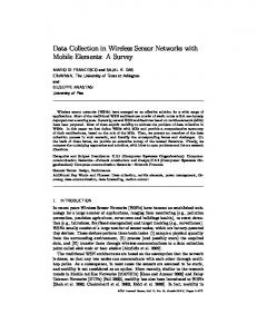
to exchange these information in order to infer current fault severity. More specifically, We are interested in message delivery rate g ) and observed reliability  . The information is exchanged as follows. h The information exchange is started by a FEEDBACKREQUEST-MSG sent from the sensor to the sink at the end of a round. The sensor repeat sending this message until a FEEDBACK-RESPONSE-MSG is received from the sink or until this message is repeated 8i ) times. The FEEDBACK-REQUEST-MSG includes the number of items sent from the sensor kjml , the number of messages sent from the sensor  nl . Note that  nl can be different from kjml since one item may be sent multiple times. h Upon hearing FEEDBACK-REQUEST-MSG, the sink calculates g ) and  , using its knowledge of the number of items received  j ) and the #pt q number of messages received #po[q  n ) : g )  # osr ,  &  #Lt r , where  jml u . The sink then sends out FEEDBACK-RESPONSE-MSG, which contains g ) and  , either  iAv times or until FEEDBACK-ACKMSG is received. h Upon receiving FEEDBACK-RESPONSE-MSG, the sensor responds with a FEEDBACK-ACK-MSG. Figure 1 describes the communication between the server and the sensor. For example, if the sensor sent out 100 data items using 150 messages, and the server received 100 messages which contain 80 distinguished data items, Vww then the message delivery rate is yxyw {zT|} and the reliability achieved is ~ . SENSOR

SINK

FEEDBACK-REQUEST: (number of data items sent, number of messages sent)

FEEDBACK-RESPONSE: (message delivery rate, observed reliability)

FEEDBACK-ACK

Figure 1. Feedback Protocol The number of re-transmissions for feedback acknowledgment ki=v is adjusted so that the probability of the sensor receiving the feedback is above a certain threshold. Let gLi=v be the probability of sensor receiving the feedback at least once after it is transmitted  iAv times, then #L€ g i=v M;aDV;ea-g ) $ . If we would like to have g i=v >5 ,  \‡U then  i=v ƒ‚ „†… N  \^ˆ q U . We can compute the number of re… N feedback request  i ) in a similar way. transmissions‚ „†for The newly computed/received g ) and  serves as an indicator of network fault severity for the next round, where parameters such as ki=v , ki ) are computed. However, it

is still possible for those feedback messages to get lost, we therefore enforce a timeout mechanism. In other words, if no feedback message is received within certain time duration, we use the parameters of the previous round.

2.2. Re-Transmission Based Plan The feedback message described above provides an indicator of current network fault rate. Let g i be the probability that a transmitted item will not reach the sink if it is sent once, then gLi-‰;aDg ) . In the presence of failure in the sensor network, data needs to be re-transmitted in order to guarantee the expected reliability. Assuming that gŠi is approximately constant within a round, the expected number of items  )  reaching the sink # at least once for plan  is: 1 P *+, ) $Š V;a‹g6i Œ $m &F2  We aim to . design an optimal transmission plan  which minimizes  $ while maintaining that *+,Ž)  $ 5 . Assuming that we have a transmission plan, in which an item is sent either  times, or k9{; times. Let 8 be the number of items that are sent out  times, and ‘ E  be the number of items that are sent out  9’; times, then  E   *+4 )  $ŠHk C V;a“g i $s9b4_adkK$ C y;”a‹g i $ (1) We now need to determine the optimal  , which should meet the following statement: the expected number of items received should be less than  can be received if all  items are transmitted  times, and it should be at least  if all  items are transmitted  9•; times. In other words,   E   C y;0aŽg i $ 7  c  C V;IaŽg i $ . From this, we get # Z # Z –F—˜ –F—˜ y;”a # $ V;a # $ c 7 –F—˜ –F—˜ a™;   g i g i #LZ –3—}˜ y;a # $ –F—˜ a5;œT i.e., 8›š gLi We also need to derive the 8   . From Equation( 1) and *+4()  $ 5k , we get  E  k 0a‹ C y;adg i $   c   E   g i a g i d  E   a‹ C V;a‹g i $ i.e.,k6Ÿž (2)  E   g i a‹g i   We have proved, via the following lemma, that this transmission plan is the optimal one.

$ { , the cost Lemma: For a plan  with *+4Ž)  6 is minimized only if ¡ ']£¢‘¤-¥T;†`¦!"!m“§¨