Shubha Kadambe and Cindy Daniell. HRL Laboratories, LLC. 3011 Malibu Canyon Road, Malibu CA 90265, USA. E-mail: {skadambe,daniell}@hrl.com.
Sensor/Data Fusion Based on Value of Information 1 Shubha Kadambe and Cindy Daniell HRL Laboratories, LLC 3011 Malibu Canyon Road, Malibu CA 90265, USA E-mail: {skadambe,daniell}@hrl.com Abstract - Spatially distributed network of inexpensive, small and smart nodes with multiple onboard sensors is an important class of emerging networked systems for various applications. Since this network of sensors has to operate efficiently in adverse environments, it is important that these sensors process information efficiently and share information such that the decision accuracy is improved. One way to address this problem is to measure the value of information obtained from multiple sensors on the same sensor node as well as from the neighboring nodes and fuse that information if value is added in terms of improvement in decision accuracy. In this paper, the measures that are developed for assessing the value of information are described. These measures are then used in making a decision of fusing either features or data from multiple sensors and neighboring nodes. While making this decision whether the value is added by fusing the information, is verified by conditioning it on improving the decision accuracy. The measures and value added are verified by using real data collected at Twentynine Plams, CA, USA and in the context of target detection and classification. From the results of improvement in classification accuracy and probability of detection reported in this paper, it can be seen that the utilization of measure of value of information while fusing helps in improving the decision accuracy significantly. Keywords: Value of information, measures of value, mutual information, decision accuracy, sensor/data fusion.
1
Introduction
Spatially distributed network of inexpensive, small and smart nodes with multiple onboard sensors is an important class of emerging networked systems for various defense and commercial applications. Since this network of sensors has to operate efficiently in 1
© 2003 HRL Laboratories, LLC. All Rights Reserved
25
adverse environments using limited battery power and resources, it is important that these sensors process information efficiently and share information such that the decision accuracy is improved. In this paper, this is addressed by developing measures that assess the value of information obtained from multiple sensors on board on a node and from the neighboring nodes by conditioning it on improvement in the decision accuracy. If the information obtained from other sensor types on a node and/or from the neighboring nodes do improve the decision accuracy then the information is fused. In our study, information is obtained in the form of features (for classification) or data (for detection). In [1-2] we have developed a general information theoretic based metric that can be used in any kind of sensor selection and data fusion. However, while analyzing the real data with respect to a classifier and a detector we observed that the correlation between the metric of value of information and the decision accuracy depend on the type of a classifier or a detector. Hence, we think that mutual information metric may not work always. Therefore, in this paper, we have developed several measures and studied them systematically with respect to one type of classifier and a detector. To our knowledge this value of information based fusion is not studied by others and is the significant contribution of this paper. In [3], the author shows that in general by fusing data from selective sensors the performance of a network of sensors can be improved. However, this study does not describe specific novel measures for value of information and data fusion based on the assessed value unlike in this paper. In [4], techniques to represent Kalman filter state estimates in the form of information – Fisher and Shannon entropy are provided. In such a representation it is straightforward to separate out what is new information from what is either prior knowledge or common information. This separation
procedure is used in decentralized data fusion algorithms that are described in [5]. This is different from our paper in that we have developed measures for value of information and perform sensor/data fusion if the added value is in terms of improving the decision accuracy. The rest of the paper is organized as follows: In the next section details of measures that we have developed are described. Section 3 provides a brief description of the classifier and the detector that we have used in our study for the purposes of verification of the measures and data/sensor fusion. Section 4 provides the details of real data that we use in this study, the experimental setup and results. In section 5, we conclude and provide future research directions.
2
Measures of value of information
Mutual information:
Entropy is a measure of uncertainty. Let H(x) be the entropy of previously observed x events. Let y be a new event. We can measure the uncertainty of x after including y by using the conditional entropy which is defined as:
H (x y ) = H ( x , y ) − H ( y ) with
the
property
(1)
0 ≤ H (x y ) ≤ H (x ). The
conditional entropy H(x|y) represents the amount of uncertainty remaining about x after y has been observed. If the uncertainty is reduced then there is information gained by observing y. Therefore, we can measure the value of y by using conditional entropy. Another measure that is related to conditional entropy that one can use is the mutual information I(x,y) which is a measure of uncertainty that is resolved by observing y and is defined as:
I(x,y) = H (x) − H (x y ).
2.1.1
An example of value of information using mutual information as a metric
Let A = {ak} k = 1, 2,… be the set of features from sensor 1 and let B = {bl} l = 1, 2,… be the set of features from sensor 2 on the same node. Let p(ai) be the probability of feature ai. Let H(A), H(B) and H(A|B) be the entropy corresponding to sensor 1, sensor 2 and sensor 1 given sensor 2, respectively, and they are defined as [6]: 1 , ( ) p a k k H ( A B ) = H ( A , B ) − H ( B ) = ∑ p (b l )H ( A b l H (A ) =
∑ p (a ) log k
)
(3)
l
This section describes the measures of value of information that we have developed. Even though the mathematics of the metrics described below are not novel, the usage of metrics in the context of verifying value of information with respect to improving the decision accuracy (e.g., classification accuracy, detection accuracy) is new. 2.1
To explain how this measure can be used to measure value of information obtained from another sensor type an example is provided below.
=
∑ p (b )∑ p (a l
l
k
k
1 b l ) log p (a k b l
)
Here, H(A) the entropy corresponds to the prior uncertainty and H(A|B) the conditional entropy corresponds to the amount of uncertainty remaining after observing features from sensor 2. The mutual information that is defined as I(A, B) = H(A) – H(A|B) corresponds to uncertainty that is resolved by observing B in other words features from sensor 2. From the definition of mutual information, it can be seen that the uncertainty that is resolved basically depends on the conditional entropy. Let us consider two types of sensors. Let the set of features of these two sensors be B1 and B2, respectively. If H(A|B1) < H(A|B2) then I(A, B1) > I(A, B2). This implies that the uncertainty is better resolved by observing B1 as compared to B2. This further implies that B1 corresponds to features from a good sensor that is consistent with the features from sensor 1 and thus helps in improving the decision accuracy of sensor 1 and B2 corresponds to features from a bad sensor that is inconsistent with sensor 1 and hence, B2 should not be considered. Note that even though in the above example only two sensor nodes are considered for simplicity, this measure or metric can be used in a network of more than two sensors. 2.2 Euclidean Distance Unlike mutual information, Euclidean distance does not evaluate the amount of information available from a second source. It does, however, measure the similarity between two feature sets in Euclidean
(2)
26
space. This value can then be used to determine when to fuse two sources, whether from the same node or different nodes. A simple measure, Euclidean distance is defined as:
d=
∑(ai − bi ) 2
(4)
i
where ai, bi, and i are defined in Section 2.1.1. 2.3 Correlation Correlation is also a well known measure of similarity. We use the standard measure of correlation as defined by:
ρ=
E [(a − µa )(b − µb )] E [a − µa ]E [b − µb ]
(5)
where µa and µb are the means of feature sets a and b, respectively. Note that correlation is very closely related to mutual information, I(x,y) because (2) can be rewritten as: I( x , y ) =
∑ p ( a k , b k ) log k
p (a , b ) k k p (a k ) p (b k )
.
(6)
2.4 Kullback-Liebler Distance Finally, the Kullback-Liebler (KL) distance is derived from entropy, and again is a measure of the separation of two feature sets. It is defined as: D =
∑ p ( a k ) log pp (ab k ) + ∑ p ( b k ) log k
(
k )
k
p (b ) k p (a k )
.
(7)
3
Review of Algorithms used for verification
The above described metrics are used to measure the value of information obtained from other sources such as multiple sensors on a single node and from the neighboring nodes in the context of target detection and classification. For target detection, energy based detector was used and for classification, maximum likelihood based classifier was used. As mentioned before the value of information is in terms of improvement in the decision accuracy which corresponds to classification accuracy for a classifier and detection accuracy or probability of detection for a detector. Note that in this study, we did not develop a classifier or a detector; however, used those developed by others since the goal of this study is to develop measures of value of information and verify them in terms of improvement in decision accuracy
27
when they were used to make a decision of whether to fuse information obtained from the other source or not. In the following two sections we review the classifier and the detector that were used in this study. 3.1 Maximum likelihood based classifier The classifier we used for the verification of measures of value of information in terms of improving the decision accuracy is a maximum likelihood based classifier developed by the University of Wisconsin [7] as part of DARPA’s sensor information technology (SensIT) program. For a given training features and target labels a Gaussian mixture model is determined during the training phase of the classifier. During testing the distance between the test feature vector and ith class Gaussian mixture is computed. This corresponds to negative log likelihood. Then a priori probability is used to obtain the maximum a posterior classification. The features’ set that is used here consists of twenty features from the power spectral density. This is computed using 1024 FFT. The feature set is collected by summing up the values over equal length segments of the power spectrum. For the acoustic and seismic sensors the maximum frequency used was 1000 and 200 Hz, respectively. 3.2 Energy based detector An energy based detector is also used for the verification of improvement in decision accuracy when the value of information based fusion architecture is used. This detector is developed by BAE, Austin [8]; also as part of the SensIT program. A brief description of this detector is provided below. For every block of a given signal the energy of the down sampled version of the power spectral density is computed. For the computation of the power spectral density, 1024 point FFT is used. This energy is compared with a threshold value. Whenever the energy is above the threshold it was declared that the target was detected. The threshold value is adaptively changed based on the background energy.
4
Experimental details
The above described classifier and detector, and measures of value of information and the fusion algorithm which uses these measures while deciding when to and when not to fuse information were implemented in Matlab, a product of MathWorks and were tested using real data that was collected by distributing sensor nodes along east-west and southnorth road at Twentynine Palms, CA during one of the
field tests (SITEX’02). These sensor nodes are manufactured by Sensoria. On each sensor node, three sensors - acoustic, seismic and IR sensors, a four channel data acquisition board and a processing board are available. These nodes also have
communication capabilities. For more details on the sensor node, refer to [9]. SITEX’02 data corresponds to acoustic, seismic and IR data of three vehicles – AAV, Dragon Wagon (DW) and HMMWV moving along the east-west and north-south road as shown in Figure 1. In this figure, nodes placements are also provided. Totally twenty four nodes were considered in our experiments. We used both seismic and acoustic data from these nodes. In the next section, the classification experimental details and the results are provided and in section 4.2 the detection experiments and the results are provided. In both these sections experimental details and results are provided with and without value of information based fusion technique that was developed in this study.
4.1
Classification experiments
First, acoustic data from each node is considered. The maximum likelihood classifier is trained using only acoustic data from individual nodes. The challenges in the classification experiments are threefold: 1) when to reject a source of data, 2) when to propagate data between sequential nodes, and 3) when to share individual sensor data within the same node. Using only acoustic data, we investigated the effectiveness of the four measures of value of information outlined in Section 2 - mutual information, Euclidean distance, correlation, and Kullback-Liebler distance. In addition, we investigated two methods of using these measures. When evaluating the effectiveness of fusing two sources of data, is it better to compare the two sources with each other or with the stored training data? To answer this question, we devised several similarity measures to measure the closeness of two data sources. We calculated these measures between data at all sequential nodes. Then for each similarity measure, we computed its correlation with correct classification performance at each node. We call this the performance correlation. The average performance correlation over all nodes for each class of data using previous node similarity measures is shown in Figure 2. Next, we claculated the same similarity measures between the data at each node and the data stored in
the training sets. Again, for each similarity measure, we computed its correlation with correct classification performance at each node. The average performance correlation over all nodes for each class of data using training set similarity measures is shown in Figure 3. Inspection of Figures 2 and 3 show that the similarity measures Euclidean distance and correlation are more closely aligned with correct classification performance than either mutual information or Kullback-Liebler distance. In practice, however, we found that the Euclidean distance outperformed correlation as the determining factor in fusion decisions. Furthermore, comparing Figures 2 and 3 shows that using the training set for similarity measures is more effective than using the data from the previous node in the network. We found this to be true in practice as well. Subsequent work with the seismic data echoed the findings of the acoustic data. Note that even though we use the training data to make the fusion decision, we perform the actual data fusion with current and previous node data. 4.1.1 Rejection of bad data Sometimes one node or one sensor can have bad data, in which case we prefer to reject this data rather than classify with poor results. We investigated one way of recognizing such sources of bad data, by observing outliers in each dimension of the 20-dimensional feature vectors. First we computed the mean of the data at the node in question. The value at each dimension was then compared to the mean for that dimension of the stored training sets. If the data contained an outlier in 4 or more of the dimensions, for each of the training classes, we rejected the data. By rejecting the data, we did not fuse it with any other data, pass it on to any other node, nor even compute a classification at that source. Our method resulted in the rejection of several sources of bad data, thus improving the overall classification results as shown in Figures 4 and 5. 4.1.2 Node to node fusion The fusion decision can be made with a threshold, i.e. if the distance between two features sets is below some value, then fuse the two feature sets. The threshold value can be predetermined off-line or adaptive. We sidestep the threshold issue, however, by basing the fusion decision on relative distances. To do so, we initially assume the current node belonged to the same class (aka the target class) as the previous
28
node and employ the following definitions. Let xn be the mean vector of the current node data. Let xnf be the mean vector of the fused data at the current node. Let xc1 be the mean vector of the target training class data. Let xc2, xc3 be the mean vectors of the remaining training classes. A Euclidean distance ratio is defined as:
rdist = dc1 /min(dc2 ,dc3) ,
data, while using DW data for the seismic sensor results. In the case of the acoustic data, the mean correct classification performance across all nodes increases from 70% for independent operation to 93% with node to node fusion across the network. Similarly, the seismic correct classification performance increases from 42% to 52%.
(7)
4.1.3 Fusion between sensors After fusion from node to node of the individual sensors, we look at the benefit of fusing the acoustic and seismic sensor data at the same node. To do so, we employ the following definitions. Let rdist be defined as in (7) but with the new data types (a acoustic, s - seismic, and as – a concatenated acoustic/seismic vector). Let xa be the mean vector of the current node acoustic data after fusion from node to node. Let xs be the mean vector of the current node seismic data after fusion from node to node. Let xas = xa concatenated with xs (dumb fusion). Let xasf = smart fusion of xa with xs. Let xin be the data input to the classifier. Now, we employ two steps in the sensor fusion process as shown in the pseudocode below. First we employ a smart sensor fusion routine:
where dci is the Euclidean distance (4) between xn and xci. We then use the following pseudocode to make our fusion decisions.
if (rdist = 70%) check class_fuse; end else fuse_4class = 0; fuse_4carry = 0; if {(dc1 = 70%) | (class_seis >= 70%) | (class_as_ind >= 70%) } class_final_fuse = max (class_acst, class_seis, class_as_dumb, class_as_smart) end
There are two outcomes to the fusion decision. First we decide whether or not to fuse the data at the current node. If the current node has bad data, fusion can pull up the performance, however, we may not want to carry the bad data forward to the next node (the second fusion decision outcome). fuse_4class is a flag indicating whether or not to fuse for the current classification. fuse_4carry is a flag indicating whether or not to include data from the current node in the fused data that is carried forward. In Figures 4 and 5 we show the correct classification improvement gained by fusing from node to node for the acoustic and seismic sensors, respectively. For the acoustic sensor we show classification results from the AAV
Figure 6 shows the results of fusion at each stage. The classification performance is averaged over all the nodes for each vehicle class. The correct classification performance improves at each stage of fusion processing as shown in Table 1. The results indicate that the fusion based on value of information helps in improving the decision accuracy at each node significantly.
29
AAV
DW
HMMV
acoustic independent 70 % 58 % 46% seismic independent 72% 42 % 24% Acoustic fusion 93% 80% 69% seismic fusion 93% 52% 31% acoustic and seismic, 76% 55% 58% independent acoustic and seismic, 95% 90% 77 % with fusion Table 1: Summary of classification performance 4.2 Detection experiments For the detection experiments also both acoustic and seismic data were considered. First, only acoustic data from individual nodes were used. A threshold value was initially set which was varied adaptively based on the background energy. The power spectral density of acoustic data was computed using 1024 point FFT and it was downsampled by 8. The energy of the downsampled version of the power spectral density was computed. This energy was compared with the threshold value. If the energy was above the threshold value, it was decided that the target was detected. The time of detection and the confidence on detection were also calculated. The detection and time of detection were compared with the ground truth. If the target was detected when it is supposed to be and if the time of detection is within the region of interest then it was counted towards calculating the probability of detection. If the detection time is outside the region of interest (missed detection) and if a target was detected when it should not have been (false alarm) it was counted towards computing the probability of false alarm. The probability of detection and false alarm using only acoustic data from individual nodes without any fusion for AAV, DW and HMMWV are: 0.8824, 0.8677, 0.8382 & 0.1176, 0.1323, 0.1618, respectively. Similarly, the probability of detection and false alarm using only seismic data from individual nodes without any fusion for AAV, DW and HMMWV are: 0.8030, 0.7910, 0.5735 & 0.1970, 0.2090, 0.4265, respectively. Next, the mutual information based value of information measure was used on the energy of power
spectral density to make a decision of fusing data between sensors - acoustic and seismic on each individual node. The detector was tested using the fused data on each node. The probability of detection and false alarm were computed as described above. The probability of detection of this intelligently fused data for AAV, DW and HMMWV is: 0.9394, 0.9105 and 0.8529, respectively. The probability of false alarm is not provided here because it is equal to 1 – probability of detection since both false alarm and missed detections are combined together. These results are summarized in Figure 7 in the form of a bar graph. From this, it can be seen that the intelligent sensor data fusion based on value of information significantly improves the detection accuracy. This type of fusion especially helps in difficult data as in the case of HMMWV.
5
Conclusions
In this paper, we developed measures for value of information and we used these measures to make a decision of when to fuse information from neighboring nodes and between sensors. In the case of a detector we used this measure in the case of fusing data between sensors at present. In the future, we will also use these measures to make a decision of fusing information from neighboring nodes. In the case of classification, we have demonstrated that using these measures while fusing data between sensors and from neighboring nodes improve the classification accuracy significantly. However, our rejection algorithm is not robust at present. Our future work focuses on improving this algorithm. Our future work also focuses on further studying the mutual information based measure while fusing data between sensors and from node to node. In short, our results indicate that fusion based on value of information improves the decision accuracy – classification accuracy and probability of detection significantly.
6
References
1. S. Kadambe, ``Information theoretic based sensor discrimination for information fusion and cluster formation in a network of distributed sensors,'' in Proc. of 4th annual conference on information fusion,, Montreal, Quebec, Canada, August 7-10, 2001, pp. ThC1-19-ThC1-25. 2. S. Kadambe, ``Feature discovery and sensor discrimination in a network of distributed sensors for target tracking,'' in Proc. of IEEE workshop on
30
3.
4.
5.
6.
7.
8. 9.
Statistical signal processing, Singapore, August 68, 2001, pp. 126-129. R. Battti, “Using mutual information for selecting features in supervised neural net learning,” IEEE Trans. On Neural Network, vol. 5, no. 4, July 1994, pp. 537-550. S. C. A. Thomopoulos, “Sensor selectivity and intelligent data fusion,” Proc. Of the IEEE MIT’94, October 2-5, 1994, Las Vegas, NV, pp. 529-537. J. Manyika and H. Durrant-Whyte, Data fusion and sensor management: An information theoretic approach, Prentice Hall, 1994. Papoulis, Probability, Random variables and Stochastic Processes, Second edition, McGraw Hill, 1984, pp. 500-567. Y. Hen Wu, “Maximum likelihood based classifier,” SensIT PI meeting, Jan 15-17, 2002, Santa Fe, New Mexico. S. Beck, “Energy based detector,” SensIT PI meeting, Jan 15-17, 2002, Santa Fe, New Mexico. www.sensoria.com
Ackowledgement: This work is funded by DARPA/IXO under the contract # F30602-01-C-0192. The authors would like to thank in particular Dr. Sri Kumar for funding this work under the SensIT program.
1.2
1
0.8
0.6
0.4 distance rho of means mean of rhos mut info kullback
0.2
0
-0.2 1
1.2
1.4
1.6
1.8
2
2.2
2.4
2.6
2.8
3
Figure 2: Performance correlation of previous node data
1
0.8
0.6 0.4
0.2
0
-0.2 -0.4 distance rho kullback
-0.6
-0.8 1
1.2
1.4
1.6
1.8
2
2.2
2.4
2.6
2.8
3
Figure 3: Performance correlation of training class data
Figure 1: Sensor node distribution at Twenty nine Palms, CA
31
100 90 80
70 60 50 40 30
20 Pcc independent Pcc w/ node fusion
10 0
0
5
10
15
20
25
Figure 4: Performance of node fusion for the AAV with acoustic sensor data 100 Pcc independent Pcc w/ node fusion
90
Figure 7: Performance of a detector
80
70
60
50
40
30
20
10
0
5
10
15
20
25
Figure 5: Performance of node fusion for the DW with seismic sensor data
Figure 6: Average correct classification performance at each step in the fusion process
32