Sensor Fusion in Time-Triggered Systems - Semantic Scholar

DISSERTATION

Sensor Fusion in Time-Triggered Systems ausgefu ¨hrt zum Zwecke der Erlangung des akademischen Grades eines Doktors der technischen Wissenschaften unter der Leitung von O. Univ.-Prof. Dr. Hermann Kopetz Institut fu ¨r Technische Informatik 182 eingereicht an der Technischen Universität Wien, Fakultät fu ¨r Technische Naturwissenschaften und Informatik von Wilfried Elmenreich Matr.-Nr. 9226605 Su ¨dtirolerstraße 19, A-8280 Fu ¨rstenfeld

Wien, im Oktober 2002

...........................

Sensor Fusion in Time-Triggered Systems Sensor fusion is the combining of sensory data or data derived from sensory data in order to produce enhanced data in form of an internal representation of the process environment. The achievements of sensor fusion are robustness, extended spatial and temporal coverage, increased confidence, reduced ambiguity and uncertainty, and improved resolution. This thesis examines the application of sensor fusion for real-time applications. The time-triggered approach provides a well suited basis for building real-time systems due to its highly deterministic behavior. The integration of sensor fusion applications in a time-triggered framework supports resource-efficient dependable real-time systems. We present a timetriggered approach for real-time sensor fusion applications that partitions the system into three levels: First, a transducer level contains the sensors and the actuators. Second, a fusion/dissemination level gathers measurements, performs sensor fusion and distributes control information to the actuators. Third, a control level contains a control program making control decisions based on environmental information provided by the fusion level. Using this architecture, complex applications can be decomposed into smaller manageable subsystems. Furthermore, this thesis evaluates different approaches for achieving dependability. These approaches attack the problem at different levels. At the transducer level, we introduce a filter algorithm that performs successive measurements in order to improve the data quality of a single sensor. A different approach improves data by combining data of multiple sensors at the fusion/dissemination level. We propose two sensor fusion algorithms to accomplish this task, the systematic confidence-weighted averaging algorithm and the application-specific robust certainty grid algorithm. The proposed methods are evaluated and used in a case study featuring an autonomous mobile robot.

i

ii

Sensor Fusion in zeitgesteuerten Systemen Unter Sensor Fusion versteht man die intelligente Zusammenf¨ uhrung von Sensordaten zu einem konsistenten Bild der beobachteten Umgebung. Die Verwendung von Sensor Fusion erzielt stabiles Verhalten gegen¨ uber Störeinfl¨ ussen, eine Verbesserung des zeitlichen oder räumlichen Messbereichs, erhöhte Aussagewahrscheinlichkeit einer Messung, eindeutige Interpretationen der Daten sowie verbesserte Auflösung der Messdaten. Diese Arbeit untersucht die Integration von Sensor Fusion in Echtzeitsystemen. Echtzeitsysteme m¨ ussen auf gegebene Eingabedaten innerhalb definierter Zeitschranken reagieren. Zeitgesteuerte Echtzeitsysteme beinhalten eine globale Uhrensynchronisation und leiten sämtliche Steuersignale und Messzeitpunkte vom Fortschreiten der realen Zeit ab. Die Verf¨ ugbarkeit einer global synchronisierten Zeit erleichtert die Implementierung von Sensor-Fusion-Algorithmen, da die Zeitpunkte verteilter Beobachtungen global interpretiert werden können. In dieser Arbeit wird ein zeitgesteuerter Ansatz f¨ ur den Entwurf und die Implementierung von Sensor Fusion in Echtzeitanwendungen vorgestellt. Das vorgeschlagene Architekturmodell unterteilt eine Sensor-FusionAnwendung in drei Ebenen, die Transducerebene, die Fusionsebene und die Steuerungsebene. Die Unterteilung ermöglicht die Zerlegung einer komplexen Applikation in beherrschbare, getrennt implementierbare und wiederverwendbare Teile. Der zweite Schwerpunkt dieser Arbeit liegt bei der Erhöhung der Zuverlässigkeit von Sensordaten mittels Sensor Fusion. Um Zuverlässigkeit zu erreichen, werden unterschiedliche Ansätze f¨ ur die verschiedenen Ebenen vorgestellt. F¨ ur die Transducerebene wird ein Filter eingesetzt, welcher mehrere zeitlich hintereinanderliegende Messungen zusammenf¨ uhrt, um das Messergebnis zu verbessern. Auf der Fusionsebene werden Algorithmen vorgestellt, welche es ermöglichen, aus einer Anzahl von redundanten Messungen unterschiedlicher Sensoren ein robustes Bild der beobachteten Umgebung zu errechnen. Die Anwendung der vorgestellten Verfahren wird experimentiell am Beispiel eines selbstfahrenden Roboters demonstriert und evaluiert. Dabei wird die Umgebung des Roboters mittels Infrarot– und Ultraschallsensoren beobachtet, um selbstständig einen passierbaren Weg zwischen Hindernissen zu finden.

iii

iv

Danksagung Diese Arbeit entstand im Rahmen meiner Forschungs- und Lehrtätigkeit am Institut f¨ ur Technische Informatik, Abteilung f¨ ur Echtzeitsysteme, an der Technischen Universität Wien. Besonders danken möchte ich dem Betreuer meiner Dissertation, Prof. Dr. Hermann Kopetz, der mir die Forschungstätigkeit am Institut f¨ ur Technische Informatik ermöglichte. Er unterst¨ utzte meine Arbeit durch wertvolle Anregungen und stimulierende Diskussionen und prägte so meinen wissenschaftlichen Werdegang. Ich möchte allen meinen Kollegen und Freunden am Institut f¨ ur das angenehme Arbeitsklima danken. Das freundschaftliche Verhältnis, das wir untereinander pflegen, sowie zahlreiche fachliche Diskussionen hatten wesentlichen Einfluss auf die Qualität dieser Arbeit. Zudem danke ich Michael Paulitsch, Claudia Pribil, Peter Puschner, Thomas Galla sowie Wolfgang Haidinger, Stefan Pitzek, Philipp Peti und G¨ unther Bauer f¨ ur das gewissenhafte Korrekturlesen beziehungsweise f¨ ur wertvolle Hinweise bei der Arbeit an dieser Dissertation. Meiner Freundin Claudia Pribil möchte ich schließlich f¨ ur ihre Geduld und Unterst¨ utzung während meiner Arbeit an dieser Dissertation danken.

v

vi

Contents 1 Introduction 1.1 Related Work . . . . . . . . . . . . . . . . . . . . . . . . . . . . 1.2 Motivation and Objectives . . . . . . . . . . . . . . . . . . . . . 1.3 Structure of the Thesis . . . . . . . . . . . . . . . . . . . . . . . 2 Basic Terms and Concepts 2.1 Principles of Sensor Fusion . . . . . . . . . . . . . 2.1.1 Motivation for Sensor Fusion . . . . . . . . 2.1.2 Limitations of Sensor Fusion . . . . . . . . 2.1.3 Types of Sensor Fusion . . . . . . . . . . . 2.2 Real-Time Systems . . . . . . . . . . . . . . . . . 2.2.1 Classification of Real-Time Systems . . . . 2.2.2 Model of Time . . . . . . . . . . . . . . . 2.2.3 Real-Time Entities and Real-Time Images 2.3 Dependability . . . . . . . . . . . . . . . . . . . . 2.3.1 Attributes of Dependability . . . . . . . . 2.3.2 Means of Dependability . . . . . . . . . . 2.3.3 Impairments of Dependability . . . . . . . 2.4 Distributed Fault-Tolerant Systems . . . . . . . . 2.4.1 Fault Modelling . . . . . . . . . . . . . . . 2.4.2 Fault Tolerance through Redundancy . . . 2.4.3 Transparency, Layering, and Abstraction . 2.5 Smart Transducer Networks . . . . . . . . . . . . 2.5.1 Sensors and Actuators . . . . . . . . . . . 2.5.2 Microcontrollers for Embedded Systems . 2.5.3 Smart Transducer Interfaces . . . . . . . . 2.6 Chapter Summary . . . . . . . . . . . . . . . . .

vii

. . . . . . . . . . . . . . . . . . . . .

. . . . . . . . . . . . . . . . . . . . .

. . . . . . . . . . . . . . . . . . . . .

. . . . . . . . . . . . . . . . . . . . .

. . . . . . . . . . . . . . . . . . . . .

. . . . . . . . . . . . . . . . . . . . .

. . . . . . . . . . . . . . . . . . . . .

. . . . . . . . . . . . . . . . . . . . .

1 3 4 5 7 7 9 12 13 17 18 21 21 22 22 24 24 25 26 27 28 29 29 30 30 32

3 Sensor Fusion Architectures and Applications 3.1 Architectures for Sensor Fusion . . . . . . . . . 3.1.1 The JDL Fusion Architecture . . . . . . 3.1.2 Waterfall Fusion Process Model . . . . . 3.1.3 Boyd Model . . . . . . . . . . . . . . . . 3.1.4 The LAAS Architecture . . . . . . . . . 3.1.5 The Omnibus Model . . . . . . . . . . . 3.2 Methods and Applications . . . . . . . . . . . . 3.2.1 Smoothing, Filtering, and Prediction . . 3.2.2 Kalman Filtering . . . . . . . . . . . . . 3.2.3 Inference Methods . . . . . . . . . . . . 3.2.4 Occupancy Maps . . . . . . . . . . . . . 3.2.5 Certainty Grid . . . . . . . . . . . . . . 3.2.6 Reliable Abstract Sensors . . . . . . . . 3.3 Chapter Summary . . . . . . . . . . . . . . . . 4 Architectural Model 4.1 Design Principles . . . . . . . . . . . . . . . . 4.2 Time-Triggered Sensor Fusion Model . . . . . 4.2.1 Transducer Level . . . . . . . . . . . . 4.2.2 Fusion/Dissemination Level . . . . . . 4.2.3 Control Level . . . . . . . . . . . . . . 4.2.4 Operator . . . . . . . . . . . . . . . . . 4.3 Interfaces . . . . . . . . . . . . . . . . . . . . 4.3.1 Interface Separation . . . . . . . . . . 4.3.2 Interfaces in the Time-Triggered Sensor 4.3.3 Interface File System . . . . . . . . . . 4.4 Communication Protocol . . . . . . . . . . . . 4.4.1 Bus Scheduling . . . . . . . . . . . . . 4.4.2 Clock Synchronization . . . . . . . . . 4.5 Discussion . . . . . . . . . . . . . . . . . . . . 4.5.1 Benefits at Transducer Level . . . . . . 4.5.2 Benefits at Fusion/Dissemination Level 4.5.3 Benefits at Control Level . . . . . . . . 4.6 Chapter Summary . . . . . . . . . . . . . . .

viii

. . . . . . . . . . . . . .

. . . . . . . . . . . . . .

. . . . . . . . . . . . . .

. . . . . . . . . . . . . . . . . . . . . . . . . . . . . . . . Fusion . . . . . . . . . . . . . . . . . . . . . . . . . . . . . . . . . . . .

. . . . . . . . . . . . . .

. . . . . . . . . . . . . .

. . . . . . . . . . . . . .

. . . . . . . . . . . . . .

. . . . . . . . . . . . . . . . . . . . . . . . . . . . . . . . Model . . . . . . . . . . . . . . . . . . . . . . . . . . . . . . . . . . . .

. . . . . . . . . . . . . .

. . . . . . . . . . . . . . . . . .

. . . . . . . . . . . . . .

33 33 33 35 36 37 39 40 40 41 44 45 46 48 49

. . . . . . . . . . . . . . . . . .

51 51 53 54 56 57 57 58 58 59 62 65 65 68 68 68 69 69 70

5 Achieving Dependability by Sensor Fusion 5.1 Systematic versus Application-Specific Approach 5.2 Systematic Dependability Framework . . . . . . 5.2.1 Problem Statement . . . . . . . . . . . . 5.2.2 Modelling of Observations . . . . . . . . 5.2.3 Sensor Representation Model . . . . . . 5.2.4 Representation of Confidence Values . . 5.2.5 Fusion Algorithms . . . . . . . . . . . . 5.3 Robust Certainty Grid . . . . . . . . . . . . . . 5.3.1 Problem Statement . . . . . . . . . . . . 5.3.2 Robust Certainty Grid Algorithm . . . . 5.4 Chapter Summary . . . . . . . . . . . . . . . .

. . . . . . . . . . .

6 Case Study Setup 6.1 Problem Statement . . . . . . . . . . . . . . . . . 6.1.1 Hardware Constraints . . . . . . . . . . . 6.1.2 Software Constraints . . . . . . . . . . . . 6.1.3 Real-Time Constraints . . . . . . . . . . . 6.2 Development Environment . . . . . . . . . . . . . 6.2.1 Target System . . . . . . . . . . . . . . . . 6.2.2 Programming Language . . . . . . . . . . 6.2.3 Compiler . . . . . . . . . . . . . . . . . . . 6.2.4 Programming Tools . . . . . . . . . . . . . 6.3 System Architecture . . . . . . . . . . . . . . . . 6.4 Demonstrator Hardware . . . . . . . . . . . . . . 6.4.1 Electrical and Electromechanical Hardware 6.4.2 TTP/A Nodes . . . . . . . . . . . . . . . . 6.5 Demonstrator Software . . . . . . . . . . . . . . . 6.5.1 Infrared Sensor Filter . . . . . . . . . . . . 6.5.2 Servo Control . . . . . . . . . . . . . . . . 6.5.3 Grid Generation . . . . . . . . . . . . . . . 6.5.4 Navigation and Path Planning . . . . . . . 6.5.5 Fusion of Ultrasonic Observations . . . . . 6.5.6 Intelligent Motion Control . . . . . . . . . 6.6 Chapter Summary . . . . . . . . . . . . . . . . .

ix

. . . . . . . . . . .

. . . . . . . . . . . . . . . . . . . . .

. . . . . . . . . . .

. . . . . . . . . . . . . . . . . . . . .

. . . . . . . . . . .

. . . . . . . . . . . . . . . . . . . . .

. . . . . . . . . . .

. . . . . . . . . . . . . . . . . . . . .

. . . . . . . . . . .

. . . . . . . . . . . . . . . . . . . . .

. . . . . . . . . . .

. . . . . . . . . . . . . . . . . . . . .

. . . . . . . . . . .

. . . . . . . . . . . . . . . . . . . . .

. . . . . . . . . . .

71 71 72 72 72 75 77 78 83 83 84 89

. . . . . . . . . . . . . . . . . . . . .

91 91 91 92 92 93 93 93 94 94 95 97 97 101 104 104 105 105 106 109 110 111

7 Experiments and Evaluation 7.1 Analysis of Sensor Behavior . . . . . . . . . . 7.1.1 Raw Sensor Data . . . . . . . . . . . . 7.1.2 Sensor Filtering . . . . . . . . . . . . . 7.1.3 Fused Sensor Data . . . . . . . . . . . 7.1.4 Comparison of Results . . . . . . . . . 7.2 Evaluation of Certainty Grid . . . . . . . . . . 7.2.1 Free Space Detection . . . . . . . . . . 7.2.2 Dead End Detection . . . . . . . . . . 7.2.3 Typical Situation with Three Obstacles 7.3 Discussion and Chapter Summary . . . . . . .

. . . . . . . . . .

. . . . . . . . . .

. . . . . . . . . .

. . . . . . . . . .

. . . . . . . . . .

. . . . . . . . . .

. . . . . . . . . .

. . . . . . . . . .

. . . . . . . . . .

. . . . . . . . . .

113 113 113 119 121 125 128 128 130 130 133

8 Conclusion 135 8.1 Time-Triggered Architecture for Sensor Fusion . . . . . . . . . . 135 8.2 Sensor Fusion Algorithms . . . . . . . . . . . . . . . . . . . . . 136 8.3 Outlook . . . . . . . . . . . . . . . . . . . . . . . . . . . . . . . 137 Bibliography

139

List of Publications

155

Curriculum Vitae

157

x

List of Figures 2.1 2.2 2.3 2.4 2.5

Block diagram of sensor fusion and multisensor integration Alternative fusion characterizations based on input/output Competitive, complementary, and cooperative fusion . . . Parts of a real-time system . . . . . . . . . . . . . . . . . . Dependability tree . . . . . . . . . . . . . . . . . . . . . .

. . . . .

. . . . .

. . . . .

10 14 16 18 23

3.1 3.2 3.3 3.4 3.5 3.6

JDL fusion model . . . . . . . . . . The waterfall fusion process model The Boyd (or OODA) loop . . . . . LAAS Architecture . . . . . . . . . The omnibus model . . . . . . . . . Smoothing, filtering, and prediction

. . . . . .

. . . . . .

. . . . . .

. . . . . .

. . . . . .

. . . . . .

. . . . . .

34 36 37 38 39 41

4.1 4.2 4.3 4.4 4.5 4.6 4.7 4.8

Data flow in the time-triggered sensor fusion model . The three interfaces to a smart transducer node . . . Nested configuration with intelligent control interface Interface file system as temporal firewall . . . . . . . Physical network topology . . . . . . . . . . . . . . . Logical network structure . . . . . . . . . . . . . . . Communication in TTP/A . . . . . . . . . . . . . . . Recommended TTP/A Schedule . . . . . . . . . . . .

. . . . . . . .

. . . . . . . .

. . . . . . . .

. . . . . . . .

. . . . . . . .

. . . . . . . .

54 58 61 63 64 65 66 67

5.1

Sensor fusion layer converting redundant sensor information into dependable data . . . . . . . . . . . . . . . . . . . . . . . . . . . Structure of fusion operator . . . . . . . . . . . . . . . . . . . . Structure of sensor fusion layer . . . . . . . . . . . . . . . . . . Example for sensor behavior regarding accuracy and failure . . . Conversion function for confidence/variance values . . . . . . . Discrepancy between sensor A and sensor B due to object shape

73 74 75 76 77 85

5.2 5.3 5.4 5.5 5.6

xi

. . . . . .

. . . . . .

. . . . . .

. . . . . .

. . . . . .

. . . . . .

. . . . . .

. . . . . .

. . . . . .

5.7

Pseudocode of the AddToGrid algorithm . . . . . . . . . . . . .

6.1 6.2 6.3 6.4 6.5 6.6 6.7 6.8 6.9 6.10 6.11 6.12

System architecture of smart car . . . . . . . . . . . . Hardware parts of smart car . . . . . . . . . . . . . . Infrared sensor signal vs. distance to reflective object Timing diagram for the GP2D02 sensor . . . . . . . . Connection diagram for the GP2D02 infrared sensor . Timing diagram for the ultrasonic sensor . . . . . . . Employed TTP/A node types . . . . . . . . . . . . . Network schematic of smart car . . . . . . . . . . . . Line of sight for each position and sensor . . . . . . . Path planning . . . . . . . . . . . . . . . . . . . . . . Risk distribution scheme . . . . . . . . . . . . . . . . Example scenario for navigation decision-making . . .

7.1 7.2 7.3 7.4 7.5 7.6 7.7 7.8

Setup for individual sensor testing . . . . . . . . . . . . . . . . . 114 Sensor signal variations for a detected object and free space . . 115 Error of calibrated infrared sensor data . . . . . . . . . . . . . . 117 Probability density functions of the error for the ultrasonic sensors118 Error of filtered infrared sensor data . . . . . . . . . . . . . . . 120 Setup for sensor fusion testing . . . . . . . . . . . . . . . . . . . 122 Fusion result using data from sensors US 1 and US 2 . . . . . . . 122 Fusion result using unfiltered data from sensors IR 1, IR 2, and IR 3 . . . . . . . . . . . . . . . . . . . . . . . . . . . . . . . . . 123 Fusion result using filtered data from sensors IR 1, IR 2, and IR 3 123 Fusion result using data from sensors US 1 and US 2 and unfiltered data from sensors IR 1, IR 2, and IR 3 . . . . . . . . . . . . 124 Fusion result using data from sensors US 1 and US 2 and filtered data from sensors IR 1, IR 2, and IR 3 . . . . . . . . . . . . . . . 124 Free space detection . . . . . . . . . . . . . . . . . . . . . . . . 129 Dead end situation . . . . . . . . . . . . . . . . . . . . . . . . . 131 Parcour setup with three obstacles . . . . . . . . . . . . . . . . 132

7.9 7.10 7.11 7.12 7.13 7.14

xii

. . . . . . . . . . . .

. . . . . . . . . . . .

. . . . . . . . . . . .

. . . . . . . . . . . .

. . . . . . . . . . . .

. . . . . . . . . . . .

86 96 98 99 99 100 101 102 103 106 108 108 109

List of Tables 2.1

Comparison between C3 I and embedded fusion applications . . .

13

4.1 4.2

Properties of transducer, fusion/dissemination, and control level Elements of a RODL entry . . . . . . . . . . . . . . . . . . . . .

55 67

5.1 5.2

Conversion table for 16 different levels of confidence . . . . . . . Examples for grid cell updates . . . . . . . . . . . . . . . . . . .

78 87

6.1

Relation between measurement range and confidence for the ultrasonic sensors . . . . . . . . . . . . . . . . . . . . . . . . . . . 110

7.1 7.2 7.3 7.4 7.5

115 116 118 119

Sensor constants determined during calibration . . . . . . . . . Quality of calibrated infrared sensor data . . . . . . . . . . . . . Quality of calibrated ultrasonic sensor data . . . . . . . . . . . . Filtered sensor data . . . . . . . . . . . . . . . . . . . . . . . . . Performance of the fault-tolerant sensor averaging algorithm for the examined sensor configurations . . . . . . . . . . . . . . . . 7.6 Performance of the confidence-weighted average algorithm for the examined sensor configurations . . . . . . . . . . . . . . . . 7.7 Comparison of sensor data processing methods using confidenceweighted averaging as fusion method . . . . . . . . . . . . . . .

xiii

125 126 127

xiv

“Where shall I begin, please your Majesty?” he asked. “Begin at the beginning,” the King said, gravely, “and go on till you come to the end: then stop.” Alice’s Adventures in Wonderland, Lewis Carroll

Chapter 1 Introduction More and more important applications, such as manufacturing, medical, military, safety, and transportation systems, depend on embedded computer systems that interact with the real world. The many fields of application come with different requirements on such embedded systems. Especially, dependable reactive systems that have to provide a critical real-time service need carefully design and implementation. Primarily, the following aspects have to be considered: Sensor impairments: Due to limited resolution, cross-sensitivity, measurement noise, and possible sensor deprivation, an application may never depend on particular sensor information. Real-time requirements: In many embedded systems, operations have to be carried out with respect to real time. Timing failures in such applications may endanger man and machine. For example, delivering the spark at a wrong instant in an ignition control system can lead to irreversible damage of the motor of an automobile. Dependability requirements: Since embedded systems are often integrated into larger systems that depend on embedded subsystems, the embedded systems have to be designed and implemented in a way that they provide a robust service. An embedded system might have to provide a particular service even in case of failure of some of its components. Such faulttolerant behavior requires a proper design of a system with regard to the possible failure modes of its components.

1

1 Introduction

Complexity management requirements: There is often need to split a complex system, such as the software of a robot with distributed sensors and actuators, into small comprehensible subsystems in order to ease implementation and testing. The problem of sensor impairments is addressed by sensor fusion. As the name implies, sensor fusion is a technique by which data from several sensors are combined in order to provide comprehensive and accurate information. Applications of sensor fusion span a wide range from robotics, automated manufacturing, and remote sensing to military applications such as battlefield surveillance, tactical situation assessment, and threat assessment. Sensor fusion technology is still a field of intensive research. Studies in sensor fusion for computer vision and mobile robots often cite models of biological fusion such as the ones found in pigeons [Kre81] and bats [Sim95]. The apparent success of these living creatures in sensing and navigation using multisensory input indicates the great potential of the field of sensor fusion. Applications with certain real-time requirements can be built using various approaches. Due to its highly deterministic behavior, the time-triggered approach is increasingly being recognized as a well-suited basis for building distributed real-time systems. A time-triggered system consists of a set of time-aware nodes. The clocks of all nodes are synchronized in order to establish a global notion of time. Thus, the execution of communication and application tasks takes place at predetermined points in time. Except for the timing, all nodes are independent of each other. This simplifies the replication of services and maintenance tasks. Therefore, time-triggered architectures also fulfill the dependability requirements for the implementation of fault-tolerant systems using independent redundant components. Additionally, sensor fusion of redundant sensors makes an application more robust to external and internal errors. In case of failures, many sensor fusion algorithms are able to provide a degraded level of service so that the application is able to continue its operation and to provide its service. Complexity management is supported by sensor fusion as well as by timetriggered distributed systems. Sensor fusion introduces an internal representation of the environmental properties that are observed by sensors. Hence, the control application can be decoupled from the physical sensors, thus improving maintainability and reusability of the code. Moreover, time-triggered architectures support a composable design of real-time applications by breaking up complex systems into small comprehensible components. A system designer introduces interfaces that are well-defined in the value and time domain to each component. Then, all components can be implemented and tested separately. The composability principle takes care of preserving the separately

2

1 Introduction

1.1 Related Work

tested functionality of components in the overall application.

1.1

Related Work

When regarding the fields of sensor fusion and time-triggered systems separately, both are well treated in the scientific literature. The related work on sensor fusion can be structured into architectures, algorithms, and applications. Sensor fusion has many applications, which are quite different in their requirements, design, and methods. The most common architectures, like the JDL fusion model [Wal90], or the waterfall model [Mar97b] have several shortcomings that make them less applicable for particular applications. Therefore, there exists no common unique model for sensor fusion until today. The number of sensor fusion algorithms or methods is also numerous – the literature distinguishes filter algorithms (e. g., Kalman Filters [Sas00]), sensor agreement (e. g., voting, sensor selection [Gir95], fault-tolerant abstract sensors [Mar90]), world-modelling (e. g., occupancy grids [Elf89]), and decision methods (e. g., Bayes inference, Dempster-Shafer reasoning, Fuzzy logic inference [Rus94]). Related work on time-triggered systems can be found for system architectures and development (e. g., Maintainable Real-Time System [Kop93b], Time-Triggered Architecture [Sch97]), communication protocols (e. g., TTP/C [Kop99], TTP/A [Kop00], LIN [Aud99]) and many sub-aspects of distributed fault-tolerant real-time systems. However, up to date there is little related work on the combined subject of time-triggered architectures for sensor fusion. In [Lie01], Liebman and Ma tried to combine design philosophies from embedded systems design and synchronous embedded control. They proposed a hierarchical design that consists of a synchronous control application based on the time-triggered middleware language Giotto and sensor-specific code with different timing. They evaluated their design using a hardware-in-the-loop simulation of an autonomous aerial vehicle. Kostiadis and Hu proposed the design of time-triggered mobile robots that act as robotic agents for the RoboCup competition [Kos00]. Their application covers the fields of multi-agent collaboration, strategy acquisition, real-time planning and reasoning, sensor fusion, strategic decision making, intelligent robot control, and machine learning. Another research project related to sensor fusion and time-triggered systems is carried out jointly by the Department of Artificial Intelligence, the Department of Computer Architecture and Communication, and the Department of Image Processing and Pattern Recognition at the Humboldt University

3

1.2 Motivation and Objectives

1 Introduction

in Berlin.1 The objective of their project is to develop a time-triggered control architecture for instrumenting a four-legged soccer robot.

1.2

Motivation and Objectives

The main goal of this thesis is to develop a framework for sensor fusion applications in time-triggered systems. The framework will integrate sensor fusion tasks into a time-triggered architecture in order to provide a platform for dependable reactive systems. From the integration of sensor fusion tasks with a time-triggered system a synergetic effect can be expected. For instance, in system design sensor fusion will support a decomposition of tasks in thus reducing complexity. On the other hand, due to the regular timing patterns in time-triggered systems, the implementation of sensor fusion algorithms will be facilitated. As a further goal of this thesis, we will elaborate concepts for dependable sensor applications. Dependability will be achieved by using redundant sensor configurations. We will examine two approaches for implementing dependable data acquisition. Primarily, a systematic approach extends a simple application by preprocessing its inputs while the control application itself remains unchanged. The preprocessing is based on agreement protocols that rely on regularity assumptions. The expected benefits of this approach are the support for modular implementation and easy verification of the system design. Alternatively, an application-specific approach that integrates dependability operations with the application will be elaborated. The application-specific approach promises lower hardware expenses and therefore leads to reduced costs, weight, and power consumption. However, application-specific approaches usually come with increased design effort and application complexity. Our goal is to attack this complexity by taking advantage of the composable design in our framework. As an example, we will present an application-specific implementation of fault tolerance for robotic vision. As a proof of concept, we will evaluate the presented architecture and methods by means of an autonomous mobile robot. The robot shall be able to perceive its environment by means of low-cost commercial distance sensors. The robot will use this perception to create a map of the environment containing obstacles and free space. By using a path planning algorithm, the robot shall detour obstacles by choosing the most promising direction. The major challenge in this case study is the task of building an adequate map of the robot’s 1

http://www.informatik.hu-berlin.de/∼mwerner/res/robocup/index.en.html

4

1 Introduction

1.3 Structure of the Thesis

environment from inaccurate or incomplete sensor data, where the adequacy of the model is judged by its suitability for its given task, which in our case is a navigation algorithm.

1.3

Structure of the Thesis

This thesis is structured as follows: Chapter 2 introduces the basic terms and concepts that are used throughout this thesis. Section 2.1 gives a brief introduction on sensor fusion while section 2.2 is devoted to real-time systems. Thereafter, section 2.3 explains attributes, means, and impairments of dependability, whereas distributed faulttolerant systems and smart transducer networks are described in section 2.4 and 2.5. Chapter 3 provides a survey on sensor fusion architectures, methods, and applications. The first part of the survey introduces architectures and models that have been used for sensor fusion, while the second part covers sensor fusion methods and applications that are related to embedded real-time applications. In chapter 4, we describe an architectural model for sensor fusion applications in distributed time-triggered systems. Section 4.1 states the design principles that guided the design of the architectural model. Section 4.2 describes an overall model, which incorporates a smart transducer network, sensor fusion processing, and a sensor-independent environment image interface. Section 4.3 explains the interfaces and section 4.4 describes the communication within this model in detail. Chapter 5 is devoted to the introduction of two sensor fusion approaches for achieving dependability. Section 5.1 discusses two alternative approaches in order to accomplish this task. The first approach described in section 5.2 is based on a framework that systematically extends an application with a transparent sensor fusion layer. In contrast to this, section 5.3 uses an application-specific method that enables a robust version of the certainty grid algorithm for robotic perception. Chapter 6 outlines the design and implementation of a case study, the “smart car”. The smart car is an autonomous mobile robot that orientates itself by using measurements from various distance sensors. Sensor fusion and communication model are implemented according to the architecture presented in chapter 4. The evaluation of the proposed methods and the case study performance is summarized in chapter 7. Section 7.1 examines the sensor behavior and

5

1.3 Structure of the Thesis

1 Introduction

compares various fusion and filter configurations. Section 7.2 evaluates the certainty grid that has been generated from the sensor data. Finally, the thesis ends with a conclusion in chapter 8 summarizing the key results of the presented work and giving an outlook on what can be expected from future research in this area.

6

“Be wary of proposals for synergistic systems. Most of the time when you try to make 2 + 2 = 5, you end up with 3 . . . and sometimes 1.9.” Charles A. Fowler

Chapter 2 Basic Terms and Concepts The principles used throughout this thesis span over several fields of research. It is the purpose of this chapter to introduce the concepts on which the work in this thesis is based.

2.1

Principles of Sensor Fusion

There is some confusion in the terminology for fusion systems. The terms “sensor fusion”, “data fusion”, “information fusion”, “multi-sensor data fusion”, and “multi-sensor integration” have been widely used in the technical literature to refer to a variety of techniques, technologies, systems, and applications that use data derived from multiple information sources. Fusion applications range from real-time sensor fusion for the navigation of mobile robots to the off-line fusion of human or technical strategic intelligence data [Rot91]. Several attempts have been made to define and categorize fusion terms and techniques. In [Wal98], Wald proposes the term “data fusion” to be used as the overall term for fusion. However, while the concept of data fusion is easy to understand, its exact meaning varies from one scientist to another. Wald uses “data fusion” for a formal framework that comprises means and tools for the alliance of data originating from different sources. It aims at obtaining information of superior quality; the exact definition of superior quality depends on the application. The term “data fusion” is used in this meaning by the Geoscience and Remote Sensing Society1 , by the U. S. Department of Defense [DoD91], and 1

http://www.dfc-grss.org

7

2.1 Principles of Sensor Fusion

2 Basic Terms and Concepts

in many papers regarding motion tracking, remote sensing, and mobile robots. Unfortunately, the term has not always been used in the same meaning during the last years [Sme01]. In some fusion models, “data fusion” is used to denote fusion of raw data [Das97]. There are classic books on fusion like “Multisensor Data Fusion” [Wal90] by Waltz and Llinas and Hall’s “Mathematical Techniques in Multisensor Data Fusion” [Hal92] that propose an extended term, “multisensor data fusion”. It is defined there as the technology concerned with the combination of how to combine data from multiple (and possible diverse) sensors in order to make inferences about a physical event, activity, or situation [Hal92, page ix]. However, in both books, also the term “data fusion” is mentioned as being equal with “multisensor data fusion” [Hal92]. To avoid confusion on the meaning, Dasarathy decided to use the term “information fusion” as the overall term for fusion of any kind of data [Das01]. The term “information fusion” had not been used extensively before and thus had no baggage of being associated with any single aspect of the fusion domain. The fact that “information fusion” is also applicable in the context of data mining and data base integration is not necessarily a negative one as the effective meaning is unaltered: information fusion is an all-encompassing term covering all aspects of the fusion field (except nuclear fusion or fusion in the music world). A literal definition of information fusion can be found at the homepage of the International Society of Information Fusion2 : Information Fusion encompasses theory, techniques and tools conceived and employed for exploiting the synergy in the information acquired from multiple sources (sensor, databases, information gathered by human, etc.) such that the resulting decision or action is in some sense better (qualitatively or quantitatively, in terms of accuracy, robustness, etc.) than would be possible if any of these sources were used individually without such synergy exploitation. By defining a subset of information fusion, the term sensor fusion is introduced as: Sensor Fusion is the combining of sensory data or data derived from sensory data such that the resulting information is in some sense better than would be possible when these sources were used individually. 2

http://www.inforfusion.org/mission.htm

8



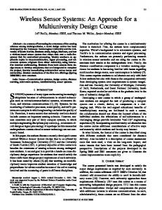
The data sources for a fusion process are not specified to originate from identical sensors. McKee distinguishes direct fusion, indirect fusion and fusion of the outputs of the former two [McK93]. Direct fusion means the fusion of sensor data from a set of heterogeneous or homogeneous sensors, soft sensors, and history values of sensor data, while indirect fusion uses information sources like a priori knowledge about the environment and human input. Therefore, sensor fusion describes direct fusion systems, while information fusion also encompasses indirect fusion processes. In this thesis we use the terms “sensor fusion” and “information fusion” according to the definitions stated before. The term “data fusion” will be avoided due to its ambiguous meaning. Since “data fusion” still is a standard term in the scientific community for earth image data processing, it is recommended not to use the stand-alone term “data fusion” in the meaning of “low-level data fusion”. Thus, unless “data fusion” is meant as proposed by the earth science community, a prefix like “low-level” or “raw” would be adequate. The sensor fusion definition above does not require that inputs are produced by multiple sensors, it only says that sensor data or data derived from sensor data have to be combined. For example, the definition also encompasses sensor fusion systems with a single sensor that take multiple measurements subsequently at different instants which are then combined. Another frequently used term is multisensor integration. Multisensor integration means the synergistic use of sensor data for the accomplishment of a task by a system. Sensor fusion is different to multisensor integration in the sense that it includes the actual combination of sensory information into one representational format [Sin97, Luo89]. The difference between sensor fusion and multisensor integration is outlined in figure 2.1. The circles S1 , S2 , and S3 depict physical sensors that provide an interface to the process environment. Block diagram 2.1(a) shows that the sensor data is converted by a sensor fusion block into a respective representation of the variables of the process environment. These data is then used by a control application. In contrast, figure 2.1(b) illustrates the meaning of multisensor integration, where the different sensor data are directly processed by the control application.

2.1.1

Motivation for Sensor Fusion

Systems that employ sensor fusion methods expect a number of benefits over single sensor systems. A physical sensor measurement generally suffers from the following problems: Sensor Deprivation: The breakdown of a sensor element causes a loss of perception on the desired object.

9



Control Application

Control Application

Internal Representation of Environment

Sensor Fusion

e .g., Voting, Averaging

S1

S2

S1

S3

S2

S3

Environment

Environment

(a) Sensor fusion

(b) Multisensor integration

Figure 2.1: Block diagram of sensor fusion and multisensor integration Limited spatial coverage: Usually an individual sensor only covers a restricted region. For example a reading from a boiler thermometer just provides an estimation of the temperature near the thermometer and may fail to correctly render the average water temperature in the boiler. Limited temporal coverage: Some sensors need a particular set-up time to perform and to transmit a measurement, thus limiting the maximum frequency of measurements. Imprecision: Measurements from individual sensors are limited to the precision of the employed sensing element. Uncertainty: Uncertainty, in contrast to imprecision, depends on the object being observed rather than the observing device. Uncertainty arises when features are missing (e. g., occlusions), when the sensor cannot measure all relevant attributes of the percept, or when the observation is ambiguous [Mur96]. A single sensor system is unable to reduce uncertainty in its perception because of its limited view of the object [Foo95]. As an example, consider a distance sensor mounted at the rear of a car in order to assist backing the car into a parking space. The sensor can only

10



provide information about objects in front of the sensor but not beside, thus the spatial coverage is limited. We assume that the sensor has an update time of one second. This is a limited temporal coverage that is significant for a human driver. Finally, the sensor does not provide unlimited precision, for example its measurements could be two centimeters off the actual distance to the object. Uncertainty arises, if the object behind the rear of the car is a small motorcycle and the driver cannot be sure, if the sensor beam hits the object and delivers a correct measurement with the specified precision or if the sensor beam misses the object, delivering a value suggesting a much different distance. One solution to the listed problems is to use sensor fusion. The standard approach to compensate for sensor deprivation is to build a fault-tolerant unit of at least three identical units with a voter [vN56] or at least two units showing fail-silent behavior [Kop90]. Fail-silent means that a component produces either correct results or, in case of failure, no results at all. In a sensor fusion system robust behavior against sensor deprivation can be achieved by using sensors with overlapping views of the desired object. This works with a set of sensors of the same type as well as with a suite of heterogeneous sensors. The following advantages can be expected from the fusion of sensor data from a set of heterogeneous or homogeneous sensors [Bos96, Gro98]: Robustness and reliability: Multiple sensor suites have an inherent redundancy which enables the system to provide information even in case of partial failure. Extended spatial and temporal coverage: One sensor can look where others cannot respectively can perform a measurement while others cannot. Increased confidence: A measurement of one sensor is confirmed by measurements of other sensors covering the same domain. Reduced ambiguity and uncertainty: Joint information reduces the set of ambiguous interpretations of the measured value. Robustness against interference: By increasing the dimensionality of the measurement space (e. g., measuring the desired quantity with optical sensors and ultrasonic sensors) the system becomes less vulnerable against interference. Improved resolution: When multiple independent measurements of the same property are fused, the resolution of the resulting value is better than a single sensor’s measurement.

11



In [Rao98], the performance of sensor measurements obtained from an appropriate fusing process is compared to the measurements of the single sensor. According to this work, an optimal fusing process can be designed, if the distribution function describing measurement errors of one particular sensor is precisely known. This optimal fusing process performs at least as well as the best single sensor. A further advantage of sensor fusion is the possibility to reduce system complexity. In a traditionally designed system the sensor measurements are fed into the application, which has to cope with a big number of imprecise, ambiguous and incomplete data streams. In a system where sensor data is preprocessed by fusion methods, the input to the controlling application can be standardized independently of the employed sensor types, thus facilitating application implementation and providing the possibility of modifications in the sensor system regarding number and type of employed sensors without modifications of the application software [Elm01c].

2.1.2

Limitations of Sensor Fusion

Evolution has developed the ability to fuse multi-sensory data into a reliable and feature-rich recognition. Nevertheless, sensor fusion is not an omnipotent method. Fowler stated a harsh criticism in 1979: One of the grabbiest concepts around is synergism. Conceptual application of synergism is spread throughout military systems but is most prevalent in the “multisensor” concept. This is a great idea provided the input data are a (sic!) good quality. Massaging a lot of crummy data doesn’t produce good data; it just requires a lot of extra equipment and may even reduce the quality of the output by introducing time delays and/or unwarranted confidence. [. . . ] It takes more than correlation and fusion to turn sows’ ears into silk purses. [Fow79, page 5] Since this has been published, many people tried to prove the opposite. Nahin and Pokoski [Nah80] presented a theoretical proof that the addition of sensors improves the performance in the specific cases for majority vote and maximum likelihood theory in decision fusion. Performance was defined as probability of taking the right decision without regarding the effort on processing power and communication. In contrast, Tenney and Sandell considered communication bandwidth for distributed fusion architectures. In their work they showed that a distributed system is suboptimal in comparison to a completely centralized processing scheme with regard to the communication effort [Ten81]. An essential criterium for the possible benefit of sensor fusion is a comprehensive set of performance measures. Theil, Kester, and Bossé presented

12



measures of performance for the fields of detection, tracking, and classification. Their work suggests measuring the quality of the output data and the reaction time [The00]. Dasarathy investigated the benefits on increasing the number of inputs to a sensor fusion process in [Das00]. Although the analysis is limited on the augmentation of two-sensor systems by an extra sensor, the work shows that increasing the number of sensors may lead to a performance gain or loss depending on the sensor fusion algorithm. It can be concluded from the existing knowledge on sensor fusion performance that in spite of the great potentials of sensor fusion slight skepticism on “perfect” or “optimal” fusion methods is appropriate.

2.1.3

Types of Sensor Fusion

The following paragraphs present common categorizations for sensor fusion applications by different aspects.

C3 I versus embedded real-time applications There exists an important dichotomy in research on sensor fusion for C3 I (command, control, communications, and intelligence) oriented applications and sensor fusion which is targeted at real-time embedded systems. The C3 I oriented research focuses primarily on intermediate and high level sensor fusion issues while onboard applications concentrate on low-level fusion. Table 2.1 compares some central issues between C3 I and embedded fusion applications (cf. [Rot91]).

Time scale Data type

Onboard fusion milliseconds sensor data

Man-machine interaction Database size Level of abstraction

optional small to moderate low

C3 I fusion seconds. . . minutes also linguistic or symbolic data frequently large to very large high

Table 2.1: Comparison between C3 I and embedded fusion applications

13



Three-Level Categorization Fusion processes are often categorized in a three-level model distinguishing low, intermediate, and high level fusion. Low-level fusion or raw data fusion (confer to section 2.1 on the double meaning of “data fusion”) combines several sources of raw data to produce new data that is expected to be more informative than the inputs. Intermediate-level fusion or feature level fusion combines various features such as edges, corners, lines, textures, or positions into a feature map that may then be used for segmentation and detection. High-level fusion, also called decision fusion combines decisions from several experts. Methods of decision fusion include voting, fuzzy-logic, and statistical methods. Categorization Based on Input/Output

Feature In Decision Out Fusion

Feature Output

Data In Feature Out Fusion

Feature Output

Data In Data Out Fusion DAI-DAO

Raw Data Output

DAI-FEO

FEI-FEO

FEI-DEO

Raw Data Level

Raw Data Input

Feature Level

Decision Output

Feature In Feature Out Fusion

Feature Input

Decision Output

DEI-DEO

Classification by Dasarathy

Figure 2.2: Alternative fusion characterizations based on input/output

14

Three-Level Classification

Decision In Decision Out Fusion

Decision Input

Decision Level

Dasarathy proposed a refined categorization based on the three-level model in [Das97]. It categorizes fusion processes derived from the abstraction level of the processes’ input and output data.



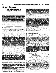
The reason for the Dasarathy model was the existence of fusion paradigms where the input and output of the fusion process belong to different levels. Examples are feature selection and extraction, since the processed data comes from the raw data level and the results belong to the feature level. For example, pattern recognition and pattern processing operates between feature and decision level. These ambiguous fusion paradigms sometimes have been assigned according to the level of their input data and sometimes according to the level of their output data. To avoid these categorization problems, Dasarathy extended the three-level view to five fusion categories defined by their input/output characteristics. Figure 2.2 depicts the relation between the three-level categorization and the Dasarathy model. Categorization Based on Sensor Configuration Sensor fusion networks can also be categorized according to the type of sensor configuration. Durrant-Whyte [DW88] distinguishes three types of sensor configuration: Complementary: A sensor configuration is called complementary if the sensors do not directly depend on each other, but can be combined in order to give a more complete image of the phenomenon under observation. This resolves the incompleteness of sensor data. An example for a complementary configuration is the employment of multiple cameras each observing disjunct parts of a room as applied in [Hoo00]. Generally, fusing complementary data is easy, since the data from independent sensors can be appended to each other [Bro98]. Sensor S2 and S3 in figure 2.3 represent a complementary configuration, since each sensor observes a different part of the environment space. Competitive: Sensors are configured competitive if each sensor delivers independent measurements of the same property. Visser and Groen [Vis99] distinguish two possible competitive configurations – the fusion of data from different sensors or the fusion of measurements from a single sensor taken at different instants. Competitive sensor configuration is also called a redundant configuration [Luo89]. A special case of competitive sensor fusion is fault tolerance which is explained in detail in section 2.4. Fault tolerance requires an exact specification of the service and the failure modes of the system. In case of a fault covered by the fault hypothesis, the system still has to provide

15



Achievements

Reliability, Accuracy

Completeness

Resulting data

Object A

Object A + B

Competitive Fusion

Complementary Fusion

Fusion

e .g., Voting

Sensors

Environment

S1

S2

S3

A

B

Emerging Views

Object C

Cooperative Fusion

e .g., Triangulation

S4

S5

C

Figure 2.3: Competitive, complementary, and cooperative fusion its specified service. Examples for fault-tolerant configurations are Nmodular redundancy [Nel90] and other schemes where a certain number of faulty components are tolerated [Pea80, Mar90]. In contrast to fault tolerance, competitive configurations can also provide robustness to a system. Robust systems provide a degraded level of service in the presence of faults. While this graceful degradation is weaker than the achievement of fault tolerance, the respective algorithms perform better in terms of resource needs and work well with heterogeneous data sources [Bak01]. An example for architectures that supports heterogeneous competitive sensors can be found in [Par91a] and [Elm02c] where confidence tags are used to indicate the dependability of an observation. Sensor S1 and S2 in figure 2.3 represent a competitive configuration, where both sensors redundantly observe the same property of an object in the environment space.

16


2.2 Real-Time Systems

Cooperative: A cooperative sensor network uses the information provided by two independent sensors to derive information that would not be available from the single sensors. An example for a cooperative sensor configuration is stereoscopic vision – by combining two-dimensional images from two cameras at slightly different viewpoints a three-dimensional image of the observed scene is derived. According to Brooks and Iyengar, cooperative sensor fusion is the most difficult to design, because the resulting data are sensitive to inaccuracies in all individual participating sensors [Bro98]. Thus, in contrast to competitive fusion, cooperative sensor fusion generally decreases accuracy and reliability. Sensor S4 and S5 in figure 2.3 represent a cooperative configuration. Both sensors observe the same object, but the measurements are used to form an emerging view on object C that could not have been derived from the measurements of S4 or S5 alone. These three categories of sensor configuration are not mutually exclusive. Many applications implement aspects of more than one of the three types. An example for such a hybrid architecture is the application of multiple cameras that monitor a given area. In regions covered by two or more cameras the sensor configuration can be competitive or cooperative. For regions observed by only one camera the sensor configuration is complementary.

2.2

Real-Time Systems

A real-time system consists of a real-time computer system, a controlled object and an operator. A real-time computer system is a computer system in which the correctness of the system behavior depends not only on the logical results of the computations, but also on the physical instant at which these results are produced [Kop97a, page 2]. Figure 2.4 depicts the parts of a real-time system. The man-machine interface consists of input devices (like keyboards, joysticks, mouse) and output devices (like displays, alarm lights, loudspeakers) that interface to a human operator. The instrumentation interface consists of the sensors and actuators that transform the physical signals of the controlled object into a processable form and vice versa. The real-time computer system must react to stimuli from the controlled object (or the operator) within a time interval specified by a deadline. If a result has utility even after its deadline has passed, the deadline is called soft, otherwise it is firm. When missing a firm deadline can have catastrophic consequences, the deadline is called hard [Kop97a]. The concept of deadlines must not be confused with fast computing. Real-time computing is not equivalent to

17



fast computing since the objective of fast computing is to minimize the average response time of a task, while real-time computing is concerned about the maximum response time and the difference between minimum and maximum response time, the so-called jitter [Sta88a]. An important aspect of real-time computing is a concise analysis of the real-time system. Katara and Luoma examined methods for determining the collective behavior of embedded real-time systems [Kat01]. They suggest that for a concise analysis it is necessary not only to regard the real-time computer system but also the properties of the environment and the operator. Real-Time System Man-Machine Interface

Instrumentation Interface

Actuators

Real-Time Computer System Operator

Nondeterministic Behavior

Sensors

Controlled Object Deterministic Behavior in Value and Time Domain

Continuous Phenomenon

Figure 2.4: Parts of a real-time system

2.2.1

Classification of Real-Time Systems

Kopetz presented a set of classifications for real-time systems in [Kop97a]. The distinction is based on the characteristics of the application (e. g., by the consequences of missing a timing requirement or the systems behavior upon failures) and on factors depending on the design and implementation of the realtime computer system (e. g., the method of system activation or assumptions regarding system response times).

18



Hard versus Soft Real-Time Systems Depending on the possible consequences of a missed deadline, hard and soft real-time systems can be distinguished. Hard real-time systems are characterized by the fact that severe consequences will result if logical or timing correctness properties are not satisfied [Sta88b]. Hard real-time systems have at least one hard deadline. Soft real-time systems are expected to deliver correct results within specified time intervals, but in contrast to hard real-time systems no severe consequences or catastrophic failures arise from missing those timing requirements. This thesis focuses on hard real-time systems. As an example for a hard real-time system, imagine a fly-by-wire or an anti-lock breaking system that interacts between a pilot or driver and a physical phenomenon. The requirement on that real-time system is that each user activity is converted to the intended change of the controlled object in the physical environment within a certain time interval. In this scenario an unexpected delay can lead to catastrophic consequences. Fail-Safe versus Fail-Operational The reaction of a system upon a critical failure is determined by application requirements. Fail-safe paradigm: This model depends on the existence of a safe state that the system can enter upon occurrence of a failure. The existence of such a fail-safe state depends on the application. In fail-safe applications, the real-time computer system must provide a high error-detection coverage. Fail-operational paradigm: If a safe state cannot be identified for a given application, the system has to be fail-operational. Fail-operational realtime systems are forced to provide at least a specified minimum level of service for the whole duration of a mission. An example for a fail-operational real-time system is a flight control system aboard an aeroplane. In contrast, a mobile robot operating on the ground usually will be able to quickly enter its safe state by stopping its propulsion, thus representing a fail-safe real-time system.

19



Event-Triggered versus Time-Triggered A trigger is an event that initiates some action like the execution of a task or the transmission of a message [Kop93a]. The services delivered by a real-time computer system can be triggered in two distinct ways: Event-triggered systems: In an event-triggered system all activities are initiated by the occurrence of events either in the environment or in the real-time computer itself. Time-triggered systems: A time-triggered system derives all the activation points from the progression of physical time. In [Kop93a], Kopetz compares the time-triggered and the event-triggered approach with respect to the temporal properties and issues of predictability, testability, resource utilization, extensibility, and assumption coverage. Timetriggered systems require an increased effort in the design phase of the system, but provide an easier verification of the temporal correctness. In event-triggered systems, it is generally difficult to make predictions about the system behavior in peak load scenarios. In this thesis, we have chosen to use an architecture that follows the timetriggered paradigm. Chapter 4 presents a time-triggered architecture for sensor fusion applications. Guaranteed Response versus Best Effort In a hard real-time system, each real-time task must be completed within a prespecified period of time after being requested. If any task fails to complete in time, the entire system fails. In order to validate a hard-real time system, it is required to ensure that all response times will always be met. Depending on the fact if such a promise can be made, systems can be distinguished into: Systems with guaranteed response are validated to hold their specified timing even in case of peak load and fault scenarios. Guaranteed response systems require careful planning and extensive analysis during the design phase [Kop97a]. Systems with best-effort design do not require a rigorous specification of load and fault scenarios. It is though very difficult to establish that such a system operates correctly in rare event scenarios [Kop97a]. In contrast to the distinction between hard and soft real-time systems, the difference between guaranteed response and best-effort systems is a property of the real-time computer system and not the real-time application.

20


2.2.2


Model of Time

For most real time applications it is sufficient to model time according to Newtonian physics [Kop02]. Hence, time progresses along a dense timeline, consisting of an infinite set of instants from past to future. An event is the observation of a state made at a particular instant. The difference between two instants is considered as a duration or an interval. Clock synchronization is concerned with bringing the time of clocks in a distributed network into close relation with respect to each other. A measure for the quality of clock synchronization are precision and accuracy. Precision is defined as the maximum offset between any two clocks in the network during an interval of interest. Accuracy is defined as the maximum offset between any clock and an absolute reference time. The finite precision of the global time and the digitalization error make it impossible to guarantee that two observations of the same event will yield the same timestamp. Kopetz [Kop92] provided a solution to this problem by introducing the concept of a sparse timebase. In this model the timeline is partitioned into an infinite sequence of alternating intervals of activity and silence. The architecture must ensure that significant events, such as the sending of a message or the observation of an event, occur only during an interval of activity. Events occurring during the same segment of activity are considered to have happened at the same time. If certain assumptions about the clock synchronization hold, events that are separated by at least one segment of silence can be consistently assigned to different timestamps for all clocks in the system. While it is possible to restrict all event occurrences within the sphere of control of the real-time computer system to these activity intervals, this is not possible for events happening in the environment, as for example, perceived by a sensor. Such events always happen on a dense timebase and must be assigned to an interval of activity by an agreement protocol in order to get a system-wide consistent perception of when an event happened in the environment [Kop02].

2.2.3

Real-Time Entities and Real-Time Images

The dynamics of a real-time application are modelled by a set of relevant state variables, the real-time entities that change their state as time progresses. Examples of real-time entities are the flow of a liquid in a pipe, the setpoint of a control loop or the intended position of a control valve. A real-time entity has static attributes that do not change during the lifetime of the real-time entity, and dynamic attributes that change with time. Examples of static attributes are the name, the type, the value domain, and the maximum rate of

21

2.3 Dependability


change. The value set at a particular instant is the most important dynamic attribute. Another example of a dynamic attribute is the rate of change at a chosen instant. The information about the state of a real-time entity at a particular instant is captured by the notion of an observation. An observation is an atomic data structure Observation = < Name, tobs , Value > consisting of the name of the real-time entity, the instant when the observation was made (tobs ), and the observed value of the real-time entity. A real-time image is a temporally accurate picture of a real-time entity at instant t, if the duration between the time of observation and the instant t is less than the accuracy interval dacc , which is an application specific parameter associated with the given real-time entity. A real-time image is thus valid at a given instant if it is an accurate representation of the corresponding real-time entity, both in the value and the time domain. While an observation records a fact that remains valid forever (a statement about a real-time entity that has been observed at an instant), the validity of a real-time image is time-dependent and is invalidated by the progression of real-time.

2.3

Dependability

Dependability of a computer system is defined as the trustworthiness and continuity of computer system service such that reliance can justifiably be placed on this service [Car82, page 41]. The service delivered by a system is its behavior as it is perceived by another system (human or physical) that interacts with the former [Lap92]. According to Laprie, dependability can be seen from different viewpoints: attributes, means, and impairments. Figure 2.5 depicts this dependability tree, which is described by the following sections.

2.3.1

Attributes of Dependability

Dependability can be described by the following five attributes: Availability is dependability with respect to the readiness for usage. The availability A(t) of a system is defined by the probability that the system is operational at a given point in time t. Reliability is dependability with respect to the continuity of service. The reliability R(t) of a system is the probability that the system is operational during a given interval of time [0, t).

22


Impairments

2.3 Dependability

Faults Errors Failures

Procurement Dependability

Means Validation

Attributes

Fault Prevention Fault Tolerance Fault Removal Fault Forecasting

Availability Reliability Safety Maintainability Security

Figure 2.5: Dependability tree Safety is dependability with respect to the avoidance of catastrophic consequences. The safety S(t) of a system is the probability that no critical failure occurs in a given interval of time [0, t). Maintainability is a measure of the time required to repair a system after the occurrence of a benign failure. Kopetz [Kop97a] quantifies maintainability with the probability M (d) that the system is restored within the duration d after failure. There is a fundamental design conflict between reliability and maintainability, since a maintainable design would imply a system composed of small replaceable units connected by serviceable interfaces. In contrast, serviceable interfaces, for example plug connections, have a significantly higher physical failure rate than non-serviceable interfaces [Kop97a]. Security encompasses the attributes confidentiality and integrity. Confidentiality is dependability with respect to the prevention of unauthorized disclosure of information. Integrity is dependability with respect to the prevention of unauthorized modifications of information. Security differs from the other four attributes in the way that it is usually not possible to quantify security.

23

2.3 Dependability

2.3.2


Means of Dependability

The means of dependability are subdivided into two groups: Procurement are means for dependability aimed at the ability of a system to provide a service complying to the system specification. There are two means for dependability procurement, fault prevention and fault tolerance. Fault prevention aims at preventing the occurrence or introduction of faults. Fault tolerance encompasses methods and techniques that enable the system to fulfill its specification despite the presence of faults. Validation describes means for dependability for gaining confidence that the system is able to deliver a service complying to the system specification. These means include fault removal and fault forecasting. Fault removal aims at reducing the presence, number, and seriousness of faults, while fault forecasting is a mean to estimate the present number, the future incidence, and the consequence of faults [Pal00].

2.3.3

Impairments of Dependability

In this context, impairments are undesired circumstances that affect the system’s dependability. Laprie distinguishes three types of impairments: faults, errors, and failures. Faults are the causes of an error. A fault might also be the consequence of the failure of another system interacting with the considered system. Faults can be classified by fault nature (chance and intentional faults), by perception (physical and design faults), by fault boundaries (internal and external faults), by origin (origin in the development or faults related to system operation), and the fault persistence (transient and permanent faults). Errors are unintended states of a computer system caused by a fault. Kopetz [Kop97a] distinguishes transient errors that exist only for a short interval of time and permanent errors, that remain in the system until the system state is fixed by an explicit repair action. Thus, it depends on the system properties like self-stabilization or automatic repair capabilities whether an error is considered transient or permanent. Failures denote the deviation between the actual and the specified behavior of a system. The ways a system can behave in case of a failure are its failure modes which can be characterized according to three viewpoints [Lap92]:

24


2.4 Distributed Fault-Tolerant Systems

Failure Domain: Laprie distinguishes value domain failures and time domain failures [Lap92]. Failure Perception: When a system has several users, according to Laprie [Lap92], one distinguishes between consistent failures, where all system users have the same perception of a failure, and inconsistent failures, where the system users have a different perception of a failure. Inconsistent failures are also known as Byzantine failures. Failure Severities: The failure severities regard the consequences of failures (ranging from benign to catastrophic failures).

2.4

Distributed Fault-Tolerant Systems

Attiya and Welch define a distributed system as a collection of individual computing devices that can communicate with each other [Att98, page 3]. The fundamental properties of a distributed system are fault tolerance and the possibility of parallelism [Mul89]. In this thesis, we focus on the subject of fault tolerance. For most distributed systems it is unacceptable that a failure of a single node implies the failure of the whole system. Therefore, fault tolerance and graceful degradation are often desirable features of distributed systems [Ler96]. Fault tolerance introduced by redundancy can be seen as a method of competitive sensor fusion (see section 2.1.3). The definition of a distributed system by Attiya and Welch also includes centralized computer systems consisting of a mainboard with several computer chips (processor, memory, I/O driver, ...) that are connected with each other via circuit paths on the printed circuit board. However, in the context of distributed fault-tolerant systems, we restrict the definition according to Poledna [Pol94b], who states the following requirements for a system to be called distributed: Independent failures: If one of the nodes fails, the other nodes must remain operational. Failures that are covered by the fault hypothesis must not impact the system’s ability to provide its specified service [Pol94b]. Non-negligible message transmission delays: The message transmission delay for communication among the nodes is not negligible in comparison to the time between events happening at a single node [Lam78]. Unreliable communication: The connections between the individual nodes are unreliable in comparison to communication between tasks within a node [Pol94b].

25



In the following, the terms and methods of fault tolerance that are relevant for this thesis are introduced. The selection of a fault tolerance method depends mainly on the specified type and likelihood of faults. Therefore, we list a taxonomy of failure modes and present methods for fault tolerance based on redundancy.

2.4.1

Fault Modelling

The assumptions taken on the failure modes and likelihood of faults for a system are expressed in the fault hypothesis. The components of a distributed system can fail in different failure modes. A failure mode is the behavior in response to a fault or error, as perceived by the user. Poledna lists some common failure modes ordered by their severeness [Pol94b]: Byzantine or arbitrary failures: There is no restriction on the effects of failures in case of Byzantine [Lam82b] or arbitrary failures. This failure mode is also referred to as malicious or fail-uncontrolled. This failure mode includes “two-faced” behavior, i. e., the output of a failed node may be perceived inconsistently by other nodes, even if they are operating correctly. Authentification detectable byzantine failures: A node may show byzantine behavior, but is not able to forge messages of other components. That means, a component cannot lie about facts sent to it by another node [Dol83]. The output of a failed node may be perceived inconsistently by other non-failed systems. Performance failures: Nodes always deliver correct results in the value domain, but regarding the time domain, they may deliver results late or early [Pow92]. Omission failures: A special case of performance failures are omission failures, where no service is delivered. In [Ezh86], an omission is defined either as a message being infinitely late or as a “null-value” sent at the right time. However, if communication bandwidth can also be used by other partners in case of an omission, only the definition of infinitely late timing would be appropriate [Pow92]. Crash failures: A crash failure is a persistent omission failure. Thus, no output is produced at any time after a failure [Bra96]. A system whose components have crash failure semantics is considered fail-silent [Lam82a].

26



Fail-stop failures: A node shows fail-stop behavior, if it does not produce any further results at any time after a failure. The other nodes in the network are able to detect consistently that the respective system has stopped [Sch84]. A system is considered a fail-stop system, if its failures can only be stopping failures. Additionally, failure modes can be characterized by the viewpoint of the failure domain [Lap92]: Value Failure: The value of a delivered service does not comply with its specification. Timing Failure: The timing of a delivered service does not comply with its specification. The combination of value and timing failure leads to a so-called babbling idiot failures – where nodes send arbitrary messages at arbitrary points in time [Tem98]. The above classifications are used to classify the failure behavior of systems, the so-called failure semantics. A system exhibits a given failure semantic if the probability of failure modes, which are not covered by the failure semantics, is sufficiently low [Pol94b]. The assumption coverage defines the probability that the possible failure modes defined by the failure semantics prove to be true in practise conditions, given the fact the system has failed [Pow92]. The assumption coverage is a critical parameter for the design of a fault-tolerant system, since a too restrictive fault model might lead to bad assumption coverage and, thus, a failure outside the failure semantics probably might lead to a total system breakdown. On the other hand, if the assumptions about failure modes are too relaxed, the system design becomes complicated, since severe failures have to be considered. Thus, an application specific compromise between complexity and assumption coverage has to be made [Pol94b].

2.4.2

Fault Tolerance through Redundancy

As a matter of fact, every single computer system will eventually fail. Requirements for highly dependable systems can only be met, if faults are taken into account. In order to tolerate faults in a distributed system, the following two design approaches can be identified [Bau01]:

27



Hardware redundancy: The system contains redundant hardware components. For example, the system could provide several hardware units that offer the same service, thus allowing the provision of a service despite faults. Software recovery: The program is designed to be able to detect and recover from faults. Compared to the hardware redundancy approach this approach does not need extra hardware, but the time for recovery has to be taken into account. Thus, all techniques for achieving fault tolerance depend upon the application of some kind of redundancy either in space, i. e., extra hardware units are present that are not necessary to fulfill the specified service in the non-errorcase, or in time, i. e., a computation is performed several times [Bau01]. In [Lee90], Lee and Anderson further describe a distinction of static (or masking) redundancy and dynamic redundancy. For static redundancy, redundant components are used within a system so that the effects of a component failure are not perceived by the user. Thus, static redundancy does not need explicit failure detection. Dynamic redundancy affords failure detection and a reconfiguration of the system in order to remove the failed components and replace them with redundant error-free ones. Examples for static redundancy are N-modular redundancy [Nel90] or forward error correcting codes. In contrast, a parity bit or the spare tire of a car relate to dynamic redundancy. However, these two types of redundancy are not always distinguishable in redundant sensor fusion systems. Many applications do not completely mask a component’s failure, but continue to provide some kind of degraded service. For example, consider a sensor system with two sensors, each with a non-negligible setup time. Both sensors are configured to measure the same property, but they will be synchronized to alternately measure the property in order to improve temporal coverage. If one sensor fails and stops to deliver further output, the system still provides a service, however only at half speed. This behavior, also known as graceful degradation, is often intrinsic to sensor fusion systems [Cha93].

2.4.3

Transparency, Layering, and Abstraction

Transparency aims at the concealment of the separation of components in a distributed system from its user. Hence, the user perceives the system as a whole, rather than as a collection of independent components. In fault-tolerant systems, transparency can be a very useful concept. For example, consider a set of identical nodes, providing redundant services. If

28


2.5 Smart Transducer Networks

one of the nodes fails, one of the correctly operating nodes can take over, thus providing a continuous service. An system based on this service could be designed following two approaches: either in providing all redundant values to the control application, or in applying an intermediate layer that filters one correct result out of the redundant values and provides this value to the control application. Thus, in the second approach, node failures or changes in the node configuration are transparent to the control application. Thus, in our context, transparency is closely related to layering. Layering is the organization of a system into separate functional components that interact in some sequential and hierarchical way, with each layer usually having an interface only to the layer above it and the layer below it. However, true transparency is not always desirable in a distributed system and should be replaced by respective abstractions [Bau01, Lea99]. Whereas with transparency, one does not deal with details, with abstraction, one does not need to deal with details.3 Thus, abstraction still allows a view on the subjacent structures of a system, e. g., for diagnostic and maintenance purposes.

2.5

Smart Transducer Networks

With the advent of cheap and small embedded microcontrollers, it became possible to build a distributed system out of a set of sensors, actuators, and control nodes, each equipped with a microcontroller unit and a network interface.

2.5.1

Sensors and Actuators

A sensor is a device that perceives a physical property (such as heat, light, sound, pressure, magnetism, or motion) and transmits the result into a measurement that can be interpreted by the computer system. Thus, a sensor maps the value of some environmental attribute to a quantitative measurement [Bro98]. An actuator is a device for moving or controlling some environmental attribute. Since sensors and actuators are both located at the same level of abstraction (at the instrumentation interface, see figure 2.4), they are often subsumed by the term transducer. In 1982, Ko and Fung introduced the term “intelligent transducer” [Ko82]. An intelligent or smart transducer is the integration of an analog or digital sensor or actuator element, a processing unit, and a communication interface. In case of a sensor, the smart transducer transforms the raw sensor signal to a 3

Pun by Doug Lea, found in [Gue02].

29



standardized digital representation, checks and calibrates the signal, and transmits this digital signal to its users via a standardized communication protocol [Kop01b]. In case of an actuator, the smart transducer accepts standardized commands and transforms these into control signals. In many cases, the smart transducer is able to locally verify the control action and provide a feedback at the transducer interface. Smart transducer technology supports the development of transducer networks, that allow monitoring, plug-and-play configuration, and the communication of digitized transducer data over the same bus line. Such a smart transducer network provides a framework that helps to reduce the complexity and cost of large distributed real-time systems.

2.5.2

Microcontrollers for Embedded Systems

An embedded system is a computer system that is designed to perform a dedicated or narrow range of functions as part of a larger system, usually with minimal end-user or operator intervention [Mar97a]. Typically, an embedded system consists of a single microprocessor board with the programs stored in the ROM. Since the limiting factors of embedded systems are often size, cost, and power consumption, many vendors offer embedded microcontrollers which contain a processor, I/O circuitry, RAM and flashable ROM memory, and a network controller in a single unit. Embedded programmable microcontrollers range from 8-bit microcontrollers to 32-bit digital signal processors (DSPs) and 64-bit processors with RISC (Reduced Instruction Set Computer) architecture. They are used for consumer-electronics devices, kitchen appliances, automobiles, networking equipment, and industrial control systems [Mar97a]. Generally, embedded microcontrollers provide very little resources. Algorithms, e. g., for sensor fusion, often have to be tailored to the available resources of an embedded microcontroller. Especially low-cost microcontrollers featuring small amounts of program and working memory have been programmed in Assembler and C rather than in C++ or Java. Since embedded systems encompass a wide range of requirements for each problem, there exists no single language for embedded systems programming [Edw00].

2.5.3

Smart Transducer Interfaces

The design of the network interface for a smart transducer is of great importance. Transducers come in a great variety with different capabilities from different vendors. Thus, a smart transducer interface must be very generic to

30



support all present and future types of transducers. However, it must provide some standard functionalities to transmit data in a temporally deterministic manner, support a standard data format, encompass means for fault tolerance, and provide means for smooth integration into a transducer network and its application. A smart transducer interface should conform to a world-wide standard. Such a standard for a real-time communication network has been sought for a long time, but efforts to find a single agreed standard have been hampered by vendors, which were reluctant to support such a single common standard in fear of losing some of their competitive advantages [Pin95]. Hence, several different fieldbus solutions have been developed and promoted. Some of these existing solutions have been combined and standardized. In 1994, the two large fieldbus groups ISP (Interoperable Systems Project supported by Fisher-Rosemount, Siemens, Yokogawa, and others) and the WorldFIP (Flux Information Processus or Factory Instrumentation Protocol, supported by Honeywell, Bailey, and others) joined to form the Fieldbus Foundation (FF). It is the stated objective of the FF to develop a single interoperable fieldbus standard in cooperation with the International Electrotechnical Commission (IEC) and the Instrumentation Society of America (ISA). The IEC worked out the IEC 61158 standard. It is based on eight existing fieldbus solutions. However, the IEC fieldbus draft standard was not ratified at the final approval vote, following a set of controversies [Nou99]. The IEC 61158 has the great disadvantage that it still keeps a diversity of eight different solutions. The ISA, which developed the SP50 standard, and IEC committees jointly met to make the development of an international standard possible. ISA SP50 was the same committee that introduced the 4-20 mA standard back in the 1970s. Meanwhile, other standards for smart transducers were developed. The IEEE 1451.2 standard [Con00] deals with the specification of interfaces for smart transducers. An idea proposed by this standard is the specification of electronic data sheets to describe the hardware interface and communication protocols of the smart transducer interface model [Ecc98]. In December 2000 the Object Management Group (OMG) called for a proposal of a smart transducer interface (STI) [OMG00]. In response, a new standard has been proposed that comprises a time-triggered transport service within the distributed smart transducer subsystem and a well-defined interface to a CORBA (Common Object Request Broker Architecture) environment. The key feature of the STI is the concept of an Interface File System (IFS) that contains all relevant transducer data. This IFS allows different views of a system, namely a real-time service view, a diagnostic and management view, and a configuration and planning view. The interface concept encompasses a communication model for transparent time-triggered communication. This STI

31

2.6 Chapter Summary


standard [OMG02] has been adopted by the OMG in January 2002.

2.6

Chapter Summary

Sensor fusion is the combination of sensory data or data derived from sensory data in order to produce enhanced data in form of an internal representation of the process environment. The advantages of sensor fusion are robustness, extended spatial and temporal coverage, increased confidence, reduced ambiguity and uncertainty, robustness against interference, and improved resolution. Generally, sensor fusion can be classified into low-level, intermediate-level, and high-level fusion. Depending on the sensor configuration, sensor fusion can be performed complementary, competitive, or cooperative. Complementary fusion provides a spatially or temporally extended view of the environment. Competitive fusion provides robustness to a system by combining redundant information. Cooperative fusion provides an emerging view of the environment by combining non-redundant information, however the result generally is sensitive to inaccuracies in all participating sensors. This thesis focuses on real-time embedded fusion systems which are usually covered by low-level sensor fusion. A real-time system contains a real-time computer system, a process environment, and an operator. The real-time computer system must react to stimuli from the controlled object or the operator before given deadlines. This thesis focuses on hard real-time systems, which are characterized by the fact that severe consequences can result if a deadline is missed. Another desired property of a system is dependability, i. e., the property of a computer system such that reliance can justifiably be placed on the service it delivers. Dependability is an overall term that includes availability, reliability, safety, maintainability, and security. A way for achieving dependability is the design of a fault-tolerant distributed system containing redundant processing components. The design of distributed sensor systems is supported by the concept of a smart transducer. A smart transducer allows uniform access to the transducer data via a standardized interface.

32

“When you use information from one source, it’s plagiarism; When you use information from many, it’s information fusion.” Belur V. Dasarathy

Chapter 3 Sensor Fusion Architectures and Applications This chapter provides a survey of sensor fusion architectures, methods, and applications related to the subject of this thesis. The section on architectures presents various models that have been used for designing fusion systems. The section on methods and applications focuses on filtering, Bayesian reasoning, map building for mobile robots, and abstract sensors.

3.1

Architectures for Sensor Fusion

Due to the fact that sensor fusion models heavily depend on the application, no generally accepted model of sensor fusion exists until today [Bed99]. According to Kam, Zhu, and Kalata, it is unlikely that one technique or one architecture will provide a uniformly superior solution [Kam97]. In this survey, we focus on architectures which have been known for a relatively long period of time.

3.1.1

The JDL Fusion Architecture

A frequently referred fusion model originates from the US Joint Directors of Laboratories (JDL). It was proposed in 1985 under the guidance of the Department of Defense (DoD). The JDL model [Wal90] comprises five levels of data processing and a database, which are all interconnected by a bus. The five

33

3.1 Architectures for Sensor Fusion

3 Architectures and Applications

Data Fusion Domain Level 0

Source Pre-Processing

Level 1

Level 2

Level 3

Object Refinement

Situation Refinement

Threat Refinement Man-Machine Interaction

Sources Database Management System

Level 4

Process Refinement

Figure 3.1: JDL fusion model (from [Lli98]) levels are not meant to be processed in a strict order and can also be executed concurrently. Figure 3.1 depicts the top level of the JDL data fusion process model. The elements of the model are described in the following: Sources: The sources provide information from a variety of data sources, like sensors, a priori information, databases, human input. Source preprocessing (Level 0): The task of this element is to reduce the processing load of the fusion processes by prescreening and allocating data to appropriate processes. Source preprocessing has later been labelled level 0 [Bed99]. Object refinement (Level 1): This level performs data alignment (transformation of data to a consistent reference frame and units), association (using correlation methods), tracking actual and future positions of objects, and identification using classification methods. Situation refinement (Level 2): The situation refinement attempts to find a contextual description of the relationship between objects and observed events. Threat refinement (Level 3): Based on a priori knowledge and predictions about the future situation this processing level tries to draw inferences about vulnerabilities and opportunities for operation. Process refinement (Level 4): Level 4 is a meta process that monitors system performance (e. g., real-time constraints) and reallocates sensor and sources to achieve particular mission goals.

34



Database management system: The task of the database management system is to monitor, evaluate, add, update, and provide information for the fusion processes. Man-machine interaction: This part provides an interface for human input and communication of fusion results to operators and users. The JDL model has been very popular for fusion systems. Despite its origin in the military domain it can be applied to both military and commercial applications. The JDL model also has categorized processes related to a fusion system. However, the model suffers from the following drawbacks: • It is a data-centered or information-centered model, which makes it difficult to extend or reuse applications built with this model. • The model is very abstract, which makes it difficult to properly interpret its parts and to appropriately apply it to specific problems. • The model is helpful for common understanding, but does not guide a developer in identifying the methods that should be used [Lli98] – thus, the model does not help in developing an architecture for a real system. The basic JDL model has also been improved and extended for various applications. Waltz showed, that the model does not address multi-image fusion problems and presented an extension that includes the fusion of image data [Wal95]. Steinberg, Bowman, and White proposed revisions and expansions of the JDL model involving broadening the functional model, relating the taxonomy to fields beyond the original military focus, and integrating a data fusion tree architecture model for system description, design, and development [Ste99].

3.1.2

Waterfall Fusion Process Model

The waterfall model, proposed in [Mar97b], emphasizes on the processing functions on the lower levels. Figure 3.2 depicts the processing stages of the waterfall model. The stages relate to the levels 0, 1, 2, and 3 of the JDL model as follows: Sensing and signal processing correspond to source preprocessing (level 0), feature extraction and pattern processing match object refinement (level 1), situation assessment is similar to situation refinement (level 2), and decision making corresponds to threat refinement (level 3). Being thus very similar to the JDL model, the waterfall model suffers from the same drawbacks. While being more exact in analyzing the fusion process

35



Decision Making Situation Assessment Pattern Processing Feature Extraction Signal Processing Sensing

Figure 3.2: The waterfall fusion process model (from [Mar97b]) than other models, the major limitation of the waterfall model is the omission of any feedback data flow. The waterfall model has been used in the defense data fusion community in Great Britain, but has not been significantly adopted elsewhere [Bed99].

3.1.3

Boyd Model

Boyd has proposed a cycle containing four stages [Boy87]. This Boyd control cycle or OODA loop (depicted in figure 3.3) represents the classic decision-support mechanism in military information operations. Because decision-support systems for situational awareness are tightly coupled with fusion systems [Bas00], the Boyd loop has also been used for sensor fusion. Bedworth and O’Brien compared the stages of the Boyd loop to the JDL [Bed99]: Observe: This stage is broadly comparable to source preprocessing in the JDL model. Orientate: This stage corresponds to functions of the levels 1, 2, and 3 of the JDL model. Decide: This stage is comparable to level 4 of the JDL model (Process refinement).

36



Decide

Orientate

Act

Observe

Figure 3.3: The Boyd (or OODA) loop Act: Since the JDL model does not close the loop by taking the actuating part of the interaction into account, this stage has no direct counterpart in the JDL model. The Boyd model represents the stages of a closed control system and gives an overview on the overall task of a system, but the model lacks of an appropriate structure for identifying and separating different sensor fusion tasks.

3.1.4

The LAAS Architecture

The LAAS (Laboratoire d’Analyse et d’Architecture des Systèmes) architecture [Ala98] was developed as an integrated architecture for the design and implementation of mobile robots with respect to real-time and code reuse. Due to the fact that mobile robot systems often employ sensor fusion methods, we briefly discuss the elements of the LAAS architecture (depicted in figure 3.4). The architecture consists of the following levels [Ala98]: Logical robot level: The task of the logical robot level is to establish a hardware independent interface between the physical sensors and actuators and the functional level. Functional level: The functional level includes all the basic built-in robot action and perception capabilities. The processing functions, such as image processing, obstacle avoidance, and control loops, are encapsulated into separate controllable communicating modules.

37



Figure 3.4: LAAS Architecture (from [Ala98]) Execution control level: The execution control level controls and coordinates the execution of the functions provided by the modules according to the task requirements. Decision level: The decision level includes the capabilities of producing the task plan and supervising its execution while being at the same time reactive to other events from the execution control level. Depending on the application, the decision level can be composed of several layers that provide different representation abstractions and have different temporal properties. The LAAS architecture maps low-level and intermediate-level sensor fusion to modules at the functional level. High-level sensor fusion is represented in the decision level. The timing requirements are different at the decision level

38



and the functional level (confer to section 2.1.3 on the difference between C3 I and real-time applications). While the architecture provides a good means for the partitioning of large systems into modules, it does not provide an appropriate real-time communication and representation of the fused data at the levels above the functional level. In contrast to the JDL model, the LAAS architecture guides a designer well in implementing reusable modules as part of a real-time application.

3.1.5

The Omnibus Model

The omnibus model [Bed99] has been presented in 1999 by Bedworth and O’Brien. Figure 3.5 depicts the architecture of the omnibus model. Unlike the JDL model, the omnibus model defines the ordering of processes and makes the cyclic nature explicit. It uses a general terminology that does not assume that the applications are defense-oriented. The model shows a cyclic structure comparable to the Boyd loop, but provides a much more fine-grained structuring of the processing levels. The model is intended to be used multiple times in the same application recursively at two different levels of abstraction. First, the model is used to characterize and structure the overall system. Second, the same structures are used to model the single subtasks of the system. Although the hierarchical separation of the sensor fusion tasks is very so-

Decision making Soft decision fusion

Hard decision fusion

Context processing Decide

Feature extraction

Control

Act

Orientate

Pattern processing

Resource tasking

Observe Sensor data fusion

Signal processing

Sensor management

Sensing

Figure 3.5: The omnibus model (from [Bed99])

39

3.2 Methods and Applications


phisticated in the omnibus model, it does not support a horizontal partitioning into tasks that reflect distributed sensing and data processing. Thus, the model does not support a decomposition into modules that can be separately implemented, separately tested, and reused for different applications.

3.2

Methods and Applications

This section investigates on sensor fusion methods and applications that are related to this thesis.

3.2.1

Smoothing, Filtering, and Prediction

Generally, the task of a sensor is to provide information about a process variable in the environment by taking measurements. Since these measurements can be noisy and are – at least in digital systems – taken at discrete points in time, it is necessary to fuse multiple measurements to reconstruct the parameter of interest. Given an observation vector ~yk corresponding to time k, we want to estimate a process state vector ~xk+m . Depending on the time k + m, ˚ Aström and ˚ Wittenmark distinguish the following three cases [Ast84]: Smoothing (m < 0): The change of a process entity shall be reconstructed after a series of measurements has been performed. For each instant of interest, several measurements from previous, actual, and following instants are used in order to estimate the value of the process variable. While the measurements have to be recorded in real time, the smoothing algorithm can be performed offline. Filtering (m = 0): The actual state of a process entity shall be estimated by using an actual measurement and information gained from previous measurements. Usually, filtering is performed in real time. Prediction (m > 0): The actual state of a process entity shall be estimated by using a history of previous measurements. The prediction problem requires an adequate system model in order to produce a meaningful estimation. Typically, prediction is performed in real time. Figure 3.6 illustrates the different cases. Many filtering algorithms cover all three aspects. Filtering and prediction are fundamental elements of any tracking system. They are used to estimate present and future kinematic quantities such as position, velocity, and acceleration [Sar91].

40


Signal


Signal

Signal

t

k

k

Estimate

t

t

k

Estimate

Estimate

t

t

t

k-1

k

(a)

(b)

k+1

(c)

Figure 3.6: Smoothing (a), filtering (b), and prediction (c)

3.2.2

Kalman Filtering

The stochastic Kalman Filter uses a mathematical model for filtering signals using measurements with a respectable amount of statistical and systematical errors. The method was developed by Kalman and Bucy in 1960 [Kal60, Kal61]. Generally, a Kalman Filter fuses data measured in successive time intervals providing a maximum likelihood estimate of a parameter. It is also possible to relate inputs from multiple sensors to a vector of internal states containing the parameters of interest as long as there are only linear dependencies between inputs and system states [Tar99]. The filter uses a discrete-time algorithm to remove noise from sensor signals in order to produce fused data that, for example, estimate the smoothed values of position, velocity, and acceleration at a series of points in a trajectory. The standard Kalman Filter model is described by two linear equations. The first equation describes the dynamics of the system: ~xk+1 = A · ~xk + B · ~uk + w

(3.1)

where ~xk is a vector that contains the system state at time k, A is the nonsingular state transition matrix. Vector ~uk describes the input to the system at time k. The relation between the input vector ~uk and the system state vector ~xk+1 is defined by matrix B. w is a random variable that stands for the system noise, modelled as white noise ∼ N (0, Q), where Q is the covariance matrix.

41



The second linear equation describes the noisy observations of the system: ~yk = C · ~xk + v

(3.2)

where each element of vector ~yk contains a sensor observation at time k, the matrix C relates the measurements to the internal state, and v is the measurement noise, also modelled as white noise ∼ N (0, R) with the covariance matrix R. The model described by equations 3.1 and 3.2 represents a very general model. For example, if one uses the identity matrix as state transition matrix (A ≡ I) and sets the input to zero (~u ≡ ~0), the model describes the standard sensor fusion case, where some internal state of a system can be reconstructed using subsequent more or less distorted measurements [Hyö97]. Another special case is given if the desired states can be measured directly. Hence, C is equivalent to the identity matrix or a permutation matrix. The Kalman Filter is applied by doing the following steps: First an a priori estimator ~xˆk+1|k of the system state ~x for time k + 1 is computed using the best system estimation at time k (equation 3.1): ~xˆk+1|k = A · ~xˆk|k + B · ~uk

(3.3)

Then we compute the predicted error covariance matrix P for instant k + 1: Pk+1|k = A · Pk|k · AT + Q

(3.4)

and the Kalman gain matrix K: Kk+1 =

Pk+1|k · CT C · Pk+1|k · CT + R

(3.5)

Now the estimator ~xˆ can be updated by a new process observation ~yk+1 : ~xˆk+1|k+1 = ~xˆk+1|k + Kk+1 · (~yk+1 − C · ~xˆk+1|k )

(3.6)

and the new error covariance matrix Pk+1|k+1 is derived by

Pk+1|k+1 = (I − Kk+1 · C)Pk+1|k (I − Kk+1 · C)T + Kk+1 · R · KTk+1

(3.7)

where I is the identity matrix. After calculation of equation 3.7 the iteration restarts with equation 3.3 and k := k + 1.

42



For start-up initialization of the Kalman Filter, one has to provide an estimate ~xˆ0 and an estimate of its covariance P0|0 . P0|0 can be initialized with an estimated inaccurate start value, since the subsequent application of the Kalman Filter will let P approach its exact value. Since each iteration has approximately the same effort, the Kalman Filter is well-suited for real-time applications. The first field of application was aerospace engineering. It was used, for example, in the Ranger, Mariner, and Apollo missions of the 1960s. Today, Honeywell’s fault-tolerant gyro system on the Boeing 777 uses a Kalman Filter [Cip93]. Kalman Filters have often been used in the field of robotics. For instance, Wen and Durrant-Whyte applied a Kalman Filter for a robot arm that uses sonar and infrared sensors to locate a specific object [Wen92]. In mobile robotics, Kalman Filters are used for correction of localizations based on two or more different types of input [Chu01, Tar99, Fab00]. Furthermore, the Kalman Filter has been applied in control theory and image processing. Although the above described standard Kalman Filter performs well for many applications, the standard Kalman Filter approach had to be extended for several applications in order to achieve satisfying results [Wen00]. Following, some extensions to the Kalman Filter are listed: Non-linear systems: Linear modelling of the system is not always feasible. Although in many cases, linear behavior around some operating point can be assumed, there are still problems that cannot be described accurately by a linear model. Therefore, the Extended Kalman Filter (EKF) has been derived that uses non-linear stochastic difference equations for the system model [Wel01]. However, while the standard Kalman Filter is optimal for linear systems, the solution provided by the EKF is only approximate. A major shortcoming of the EKF is that the distributions of the random variables are no longer normal after undergoing their nonlinear transformations. Attacking this problem, Julier et al. published a variant of EKF that uses a different parametrization of mean and covariance values that provides more accurate results than the original EKF [Jul95]. Estimating system parameters: The statistical parameters are not always known a priori or constant over time. Hence, in this case a sophisticated version of the Kalman Filter also has to estimate the statistical parameters. ˚ Aström and Wittenmark describe an approach with time-varying matrices in [˚ Ast84]. Alternatives to least mean square optimization: The Kalman Filter approach minimizes the error using a least mean square approach. Depending on the application, other criteria, such as the H∞ norm [Sha92], perform better.

43



Reducing computational load: With respect to an implementation in embedded microcontrollers, the computational effort is of great interest. Kalman filtering requires matrix multiplication and matrix inversion. If there are no dedicated vector processing units available on the microprocessor, it is important to find efficient implementations in order to achieve adequate performance and timely results. Gan and Harris showed that in a multi-sensor environment with identical measurement matrices the measurements can be handled separately in order to get computations of lower complexity [Gan01]. In case of differing measurement matrices, using a merged input vector containing the information of all sensors is preferable. Generally, large systems can be modelled with the information form of the Kalman Filter. This variant is functionally identical, but has computational advantages for high-dimensional data [Gan01].

3.2.3

Inference Methods

Merriam Webster’s college dictionary defines inference as the act of passing from one proposition, statement, or judgment considered as true to another whose truth is believed to follow from that of the former. Inference methods are used for decision fusion, i. e., to take a decision based on given knowledge. A possible application could be the decision if the road in front of a car is blocked or free, given measurements of multiple sensors. Classical inference methods perform tests on an assumed hypothesis versus an alternative hypothesis. As a test of significance, it yields the probability that the actually observed data would be present, if the chosen hypothesis were true. However, classical inference does not support the usage of a priori information about the likelihood of a proposed hypothesis [Hal92]. This a priori probability is taken into account when using Bayesian inference, which is named after the English clergyman Thomas Bayes. In a paper published after his death in the Philosophical Transactions of the Royal Society of London [Bay63] Bayes stated the rule known today as Bayes’ theorem: P(H|E) =

P(E|H) P (H) P(E)

(3.8)

Bayes’ theorem quantifies the probability of hypothesis H, given that an event E has occurred. P(H) is the a priori probability of hypothesis H, P(H|E) states the a posteriori probability of hypothesis H. P(E|H) is the probability that event E is observed given that H is true. Given multiple hypotheses, Bayesian inference can be used for classification problems. Then, Bayes’ rule produces a probability for each hypotheses Hi .

44



Each Hi corresponds to a particular class: P(Hi |E) =

P(E|Hi ) P (Hi ) Σi P (E|Hi ) P (Hi )

(3.9)

Examples for applications based on Bayesian inference can be found in [DW90] for merging multiple sensor readings, in automatic classification of sensor inputs (e. g., the computer program AUTOCLASS [Che96] developed by the NASA), or in map building for mobile robots [Elf86]. However, when Bayesian inference is used for sensor fusion, certain drawbacks can emerge [Bro98]: One problem is the required knowledge of the a priori probabilities P(E|Hi ) and P(E), which may not always be available [Bla88]. Thus, it is often necessary to make subjective judgements on some of the probabilities. Although it is possible to use subjective probabilities [Hal92], Bayesian inference requires that all probabilities are at the same level of abstraction. Another problem arrives when different sensors return conflicting data about the environment [Bog87]. Therefore, Dempster developed the mathematical foundations for a generalization of Bayesian theory of subjective probability [Dem67]. The result was Dempster’s rule of combination, which operates on belief or mass functions like Bayes’ rule does on probabilities. Shafer, a student of Dempster, extended Dempster’s work and developed a Mathematical Theory of Evidence [Sha76]. This theory can be applied for representation of incomplete knowledge, belief updating, and for combination of evidence [Pro92]. The choice between Bayesian and Dempster-Shafer inference methods for decision algorithms is non-trivial and has been subject to heated debates over the last several years [Bue88, Dau01].

3.2.4

Occupancy Maps

An occupancy map is a usually two-dimensional raster image uniformly distributed over the robot’s working space. Each map pixel contains a binary value indicating whether the according space is free or occupied by an obstacle. There are two main perceptual paradigms for occupancy map algorithms [Hoo00]: Image → objects: In the image → objects perceptual paradigm, a predefined empty area is assumed in which the observation of objects by the sensors populate the occupancy map [And92]. Object tracking algorithms, for example triangulation [Rao93], are used to obtain the positions of the objects.

45



Image → free space: In the image → free space perceptual paradigm, one assumes a predefined occupied area in which the observation of sensors creates free space in the occupancy map. Hoover and Olsen presented an application where a set of video cameras are used to detect free space in the vicinity of a robot [Hoo00]. They use multiple viewing angles to overcome the problem of occlusion and to increase performance. However, their application depends on correct measurements from all sensors. Although the first paradigm of object tracking is the more common approach, the image → free space approach has some advantages over the image → objects approach. Hoover lists reduced complexity, (no tracking is necessary to create the map), robustness, and safety (a sensor breakdown causes a loss of perception of the free space, not on the objects) as advantages [Hoo00]. However, the occupancy map approach, as described here, suffers from a major problem regardless of the used perception paradigm: map pixels, for which either none or multiple contradicting measurements are given, can be misinterpreted since the pixels of an occupancy map cannot reflect uncertainty. This problem can be overcome by extending an occupancy map with additional information about the reliance of a pixel value – this approach is known as certainty grid.

3.2.5

Certainty Grid

A certainty grid is a special form of an occupancy map. Likewise, it is a multidimensional (typically two- or three-dimensional) representation of the robot’s environment. The observed space is subdivided into square or cube cells like in the occupancy map, but each cell now contains a value reflecting a measure of probability that an object exists within the related cell [Yen98]. The information of a cell can be “free” if the corresponding space appears to be void; or “occupied” if an object has been detected at that place. Cells not reached by sensors are in an “uncertain” state. All values of the grid are initially set to this uncertain state. Each sensor measurement creates either free space or objects in the grid. Thus, the certainty grid approach is a hybrid approach between the image → objects and the image → free space perceptual paradigms of the occupancy grid. Basically, it is assumed that the certainty grid application has no a priori knowledge on the geometry of its environment and that objects in this environment are mostly static. The effect of occasional sensor errors can be neglected, because they have little effect on the grid [Mar96]. In general, sensor information is imperfect with respect to restricted temporal and spatial coverage, limited precision, and possible sensor malfunctions

46



or ambiguous measurements. To maximize the capabilities and performance it is often necessary to use a variety of sensor devices that complement each other. Mapping such sensor measurements into the grid is an estimation problem [Elf89]. Matthies and Elfes [Mat88] propose a uniform method for integrating various sensor types. Each sensor is assigned a spatial interpretation model, which is developed for each kind of sensor, that maps the sensor measurement into corresponding cells. When sensor uncertainties are taken into account, we arrive at a probabilistic sensor model. The calculation of new grid values is usually done by Bayesian inference. Suppose that two sensors S1 and S2 give two occupancy probability values for a particular grid element cell. Using Bayes’ rule, the updated probability of the cell being occupied by an obstacle can be calculated as: P(cell.occ|S1 , S2 ) = P(S1 |cell.occ, S2 ) P (cell.occ|S2 ) (3.10) P(S1 |cell.occ, S2 ) P (cell.occ|S2 ) + P(S1 |cell.emp, S2 ) P (cell.emp|S2 ) where cell.occ and cell.emp are the probabilities of the cell being occupied or empty, respectively. Conditional independence for the two sensors is defined in the following relation: P(S1 |cell.occ, S2 ) = P(S1 |cell.occ)

(3.11)

Furthermore, we assume P(cell.occ) = 1 − P(cell.emp). Assuming, that the prior probability had been equal to 0.5 (maximum entropy assumption [Mos02]), the fusion formula can be expressed by:

P(cell.occ|S1 , S2 ) = P(cell.occ|S1 ) P (cell.occ|S2 ) (3.12) P(cell.occ|S1 ) P (cell.occ|S2 ) + (1 − P(cell.occ|S1 ))(1 − P(cell.occ|S2 )) Equation 3.12 can be extended to the case of several sensors S1 , S2 , . . . , Sn by induction. Hence, the fusion formula for n sensors can be expressed as follows: n

Y 1 −1= P(cell.occ|S1 , . . . , Sn ) i=1

47

1 −1 P(cell.occ|Si )

(3.13)



Equations 3.12 and 3.13 show fully associative and commutative behavior. Thus, the order of processing does not influence the result.

3.2.6

Reliable Abstract Sensors

The term “reliable abstract sensors” has been coined by Marzullo [Mar90], who has elaborated a method for fault tolerance in multisensor environments. The main idea in Marzullo’s work is a geometric derivation for fault masking. He defines sensors as piecewise continuous functions characterized by two parameters: shape and accuracy range. Shape defines the form taken by the uncertainty around the measurement value returned by the sensor. Since Marzullo addresses only the one-dimensional case, thus assuming that all shapes are linear. The accuracy range defines the interval that contains the true value of the measured entity. By combining measurements from single sensors, an improved abstract sensor can be built. The range of this abstract sensor is derived by finding the intersections of the ranges of the single sensors. Fault-tolerant sensor averaging [Mar90] is introduced by regarding at most t sensors to be faulty.1 Faulty sensors deliver an improper interval that may not contain the true value. Therefore, a fault-tolerant sensor averaging algorithm returns an interval that contains the true value for sure, even if arbitrary t out of 2t + 1 readings are faulty. Marzullo presents an algorithm for such a reliable abstract sensor in [Mar90, page 290]: Let I be a set of values taken from n abstract sensors, and suppose the abstract sensors are of the same physical state variable where their values were read at the same instant. T Assuming that at most t of these sensors are incorrect, calculate t,n (I) which is the smallest interval that is guaranteed to contain the correct physical value. Implementation: Let l be the smallest value contained in at least n − t of the intervals in I and h beTthe largest value contained in at least n−t of the intervals in I then t,n (I) will be the interval [l...h]. Marzullo’s original work has been extended to sensors working with any number of dimensions by Chew [Che91]. While in the linear or singledimensional case the abstract sensor will always deliver correct results for at most t faulty sensors out of 2t + 1 sensors, in the multi-dimensional case there must be at least 2tD + 1 sensors in order to tolerate t faulty sensors, where D is the number of dimensions. 1

“t” is the preferred letter in the literature for the number of faults to be tolerated. It derives from the concept of a traitor in the Byzantine Generals scenario.

48


3.3 Chapter Summary

Jayasimha [Jay94] has extended Marzullo’s work with a better detection of faulty sensors for the linear case. Both, Marzullo’s and Jayasimha’s algorithm have a run time complexity of O(n log n).

3.3

Chapter Summary

This chapter provided a survey on sensor fusion architectures, methods, and applications. There is no common model for sensor fusion applications until today, however there are a host of models that propose similar partitioning into source preprocessing, feature extraction and pattern processing, situation assessment, and decision making. All of the examined architectures have some strengths and weaknesses for the modelling of sensor fusion applications. Besides the JDL model, the waterfall model is an interesting alternative for embedded real-time fusion systems since it emphasizes on low-level fusion processing. However, like the JDL model, the waterfall model has its drawbacks, i. e., it does not guide the developer in selecting the appropriate methods for concretely designing an implementation. Moreover, many typical fusion applications have a closed control loop, thus the expression of a cyclic data processing as provided by the Boyd loop and the Omnibus model is advantageous. Only the LAAS architecture, which is originally aimed at the design of mobile robots, provides means for partitioning large systems into small reusable subsystems. The section on fusion algorithms contains some of the many existing sensor fusions methods. However, currently the Kalman Filter and Bayesian reasoning are the most frequently used tools in sensor fusion. The certainty grid for robotic vision is a nice example for a combination of complementary and competitive fusion based on Bayes’ rule. As a method for sensor agreement the fault-tolerant sensor averaging algorithm has been described.

49

3.3 Chapter Summary


50

¨ “Architektur ist die externe Außerung von dem wie wir denken, organisieren und unseren Verstand verwenden.” Unknown

Chapter 4 Architectural Model This chapter describes an architectural model for sensor fusion applications in distributed time-triggered systems. This model is used in the design of the case study in chapter 6.

4.1

Design Principles

Besides the primary goal of representing the processes of a sensor fusion application for real-time systems, our objective was to find means for complexity management. A typical sensor application with local intelligence contains a network of distributed sensors, intelligence to process the sensor data (for example by sensor fusion algorithms), a control program that takes decisions based on these sensor data, and actuators that execute the decided actions. Such an application is a complex system, which is difficult to build, to verify, to repair, and to modify. Therefore, we were looking for a framework that supports the construction of such a system. We have identified the following principles to be useful in achieving our goals: Complexity management: A good method for reducing the complexity of a system is the “divide and conquer” 1 principle, i. e., the system is parti1

This proposition is derived from the concept divide et impera that described the political strategy of the Roman Empire when conquering new territory – the defeated clans had been granted different negotiations and contracts. The original quotation cannot be assigned to a single person in the antique, however was frequently used by Trajano Boccalini in [Boc78].

51

4.1 Design Principles

4 Architectural Model

tioned into interacting subsystems. Partitioning can be applied to hardand software [Wol94]. To put these subsystems to work, they must be able to communicate with each other. The design of the communication interfaces is a critical task since the borderlines between subsystems have to be well-defined interfaces to enable composability, i. e., if each subsystem implements well-defined interfaces in the temporal and value domain, it can be guaranteed a priori that the subsystem provides its specified service also in the composite system. However, a subsystem can also be provided in form of a legacy system, i. e., an autonomous system that has been developed according to its own rules and conventions [Kop01c]. If a legacy system does not provide an appropriate interface, the introduction of an extra component, an interface system, may resolve this mismatch. The interface system will then negotiate between the legacy subsystem and the other system parts. Maintenance support: Whenever a critical component of a system fails, it is necessary to detect the faulty component, repair it, reintegrate it and ensure that the system works well again according to its specification. Hence, there is an urgent need for monitoring, diagnostics, runtime configuration, and maintenance. Monitoring and debugging of distributed embedded real-time systems differ significantly from debugging and testing programs for desktop computers, because only few interfaces to the outside world are present [Tha00]. In addition, a distributed system contains multiple locations of control, and therefore conventional break-point techniques result in an undesired modification of the timing behavior. This indeterministic effect is called the “Probe Effect” [Gai86, McD89] or the “Heisenberg Uncertainty” [Led85] applied to software. Therefore, our architecture requires a deterministic monitoring environment without intrusions on the system behavior. Generic sensor fusion methods: The survey on common sensor fusion algorithms in section 3.2 revealed that many fusion methods can be implemented in a generic way. Depending on the number and types of sensors and the data desired by the application, the generic sensor fusion methods have to be configured in order to provide the intended function. In order to accommodate that fact, we separate these generic sensor fusion tasks from sensor-dependent and application-dependent issues in our architecture. Transparent fault tolerance layer: The reliability requirements of safetycritical applications can only be met, if fault tolerance is introduced. Introduction of fault tolerance increases the complexity of the system.

52


4.2 Time-Triggered Sensor Fusion Model

This complexity can be handled by introducing a transparent fault tolerance layer that hides the presence of node replicas from the control application [Bau01]. Sensor abstraction layer: Since fault tolerance and sensor fusion are closely related, the principle of a fault tolerance layer can be extended to a sensor fusion layer at the same level of abstraction. Because sensor fusion, in contrast to sensor integration, also provides an enhanced representation of the environment data by world modelling, it allows us to abstract from the measuring instruments. Control application design: Unlike the JDL model described in section 3.1.1, we expect a model that reflects the cyclic structure that is inherent to every control system. Most control algorithms need periodical updates of control values where the update times must have low jitter. As a further requirement, the duration from performing a measurement until the execution of the control decision is usually limited to a maximum dead time and jitter by the control algorithm.

4.2

Time-Triggered Sensor Fusion Model

Most existing fusion models, as found in the literature (see section 3.1), have been very abstract when it comes to timing and communication properties. Since we aim at modelling a complex real-time system with data acquisition, fusion processing, and control decisions, we have to extend the existing approaches in order to obtain a meaningful framework. Therefore, we introduce a time-triggered sensor fusion model [Elm01b]. The model incorporates properties like cyclic processing, composable design, and introduces well-defined interfaces between its subsystems. Figure 4.1 depicts a control loop modelled by the time-triggered sensor fusion model. Interfaces are illustrated by a disc with arrows indicating the possible data flow directions across the interface. Physical sensors and actuators are located on the borderline to the process environment and are represented by circles. All other components of the system are outlined as boxes. The model distinguishes three levels of data processing with well-defined interfaces between them. The transducer level contains the sensors and actuators that interact directly with the controlled object. A smart transducer interface provides a consistent borderline to the above fusion/dissemination level. This level contains fault tolerance and sensor fusion tasks. The control level is the highest level of data processing within the control loop. The control level is fed by a dedicated view of the environment (established by transducer and fusion/dissemination level) and out-

53



Operator

Man-Machine Interface

Fault-Tolerant Image of the Environment

Fault-Tolerant Actuator Interface

Control Application

Sensor Abstraction Layer Fault Tolerance Layer

Fault Tolerance Layer

Smart Transducers Interface

Control Level

Fusion/Dissemination Level Smart Transducers Interface

Sensors

Actuators

Transducer Level

Environment Controlled Object

Figure 4.1: Data flow in the time-triggered sensor fusion model puts control decisions to a fault-tolerant actuator interface. User commands from an operator interact with the control application via the man-machine interface. The breakdown into these three levels is justified by the different tasks the three levels have to fulfill and the different knowledge necessary for designing the corresponding hard- and software. Table 4.1 describes the task and the attributes of the different levels. The following sections describe the three levels in detail.

4.2.1

Transducer Level

The sensors and actuators that physically interact with the environment establish the transducer level of the system. To support maximum modularity, the

54



Level Transducer level

Task Deliver sensor measurements, instrument actuators Fusion/Dissemina- Gather, process, tion level and represent sensor information; disseminate control decisions to actuators Control level Find a control decision, navigation and planning Operator Definition of goals

Implementer Transducer manufacturer

Knowledge Internals of sensor/actuator

System integrator

Sensor fusion algorithms, fault tolerance concepts

Application grammer

Mission goals, control theory, decision finding Conceptual model of system

—

pro-

Table 4.1: Properties of transducer, fusion/dissemination, and control level nodes are built as smart transducers. The smart transducer technology offers a number of advantages from the point of view of technology, cost, and complexity management. The task of a transducer is either to provide observations about properties of the controlled object or, in case of an actuator, execute a control value. An observation subsumes the information assigned to a measurement such as measurement value, measurement instant, and meta-information about the measurement. We have identified the following possible features of a smart transducer: Signal amplifying and conditioning: Electrically weak non-linear sensor signals can be amplified, conditioned, and transformed into digital form locally at the transducer node without any noise pickup from long external signal transmission lines [Die98]. Local fusion of measurements: Either a local transducer node has access to two or more sensor signals or the transducer is capable of using multiple measurements taken by a single sensor at different instants. Self-validation: The transducer can also provide information about the correctness and/or quality of its measurements by running self-diagnostics. If an assumption of the maximum gradient of the measured signal can be made, the sensor can monitor changes of measurements and detect abnormal behavior.

55



Conversion to standard representation: The measurement can be locally converted to standard measurement units and data types that allow a uniform representation of observations throughout the system regardless of the transducer type. Timestamping: Each measurement can be augmented by information about the instant when it has been performed. If local clock of the microcontroller is synchronized to a global time, the measurement can be assigned a timestamp of global validity. A timestamp can provide information about the ordering and the interval time between subsequent measurements. Meta-information: The transducer can also assign meta information, such as data type or confidence of measurement, to its observations. Typically, smart transducers are mass products, sold in quantities in the tens of millions. Therefore, a smart transducer must be flexible enough to be used for different applications. The implementation of a smart transducer usually supports only generic or sensor/actuator-specific tasks and comes with a host of configuration parameters. An important feature of a smart transducer is its capability of providing machine-readable self-description. Tools operating on these descriptions support system architects in the consistent configuration of smart transducers within a network. For example, a tool may access the description of a newly connected node for an easy plug-and-play-like integration of the node into the system.

4.2.2

Fusion/Dissemination Level

While each single sensor only provides a small view of the environment, it is the task of the fusion/dissemination level to integrate the measurements into a description of the environment that enables the control program to assess the situation more comprehensively. The fusion/dissemination level contains the hardware and software that act as a glue between the transducers and the control program. It creates a unified view using sensor data which is named the environment image. If required, this image is made robust to incomplete, erroneous or missing measurements by implementing a fault tolerance layer. Typical methods for the fault tolerance layer are voting or averaging. While on the sensor side of the control loop, data from multiple sensors are fused to reliable data, the task of the fault tolerance layer on the actuator side of the control loop is to create multiple instances of a control message for the redundant actuators.

56



Furthermore, the fusion/dissemination level can make use of all types of sensor fusion algorithms. Competitive fusion methods increase the robustness of the perception, while cooperative and complementary fusion provide extended and more complete views. Which algorithms are particularly used in the fusion/dissemination level depends on the available resources like processing power, working memory, and on application-specific needs at the control level.

4.2.3

Control Level

The control level contains the control intelligence to make decisions based on the world image. The control program initiates actions in order to achieve a given goal. If the fusion/dissemination level additionally provides information about the condition of the system, the control program also has to adapt its goal according to the circumstances. For example, consider an onboard automatic flight control system of an aircraft that is programmed with the target “airport” as goal. However, if the system detects that N − 1 out of a set of N redundant mission-critical sensors have already failed, it might select the nearest airport for maintenance. On the other hand, if the fusion/dissemination level is implemented in a way that hides all sensor or actuator problems from the control program, the complexity at the control level can be reduced, however at the cost of system features. Our model resolves this problem by introducing different interfaces for the real-time service and maintenance (see section 4.3.1).

4.2.4

Operator

The operator defines the goals, which the control application tries to reach. For this purpose the operator does not need a detailed understanding of the technical operation of the system. Instead, the operator follows a conceptual model of the system that allows him or her to understand the important aspects of the application and hence give the respective correct inputs to the system. For example, when driving a car, we usually do not imagine the operation of the carburetor, sparks, and cylinders in the motor when we press the accelerator pedal. However, we have a different conceptual model on accelerating and breaking, since even with the fastest cars it makes a big difference between the time (or distance) a car takes to accelerate to a particular speed and the time (or distance) the car needs to stop. Perhaps in future times, speed of a car will be controlled by a single joystick that can be pushed forward or backward, and we will switch to a conceptual model where accelerating or braking makes less difference.

57

4.3 Interfaces

4.3


Interfaces

An interface is a common boundary between two subsystems [Kop97a, page 77]. A correctly designed interface should provide an understandable abstraction to the interfacing partners. Such an interface provides essential properties and hides irrelevant details. Thereby, it eases the understanding of the component interactions and helps to control the system complexity. It only offers information of the specific services that is required by the user. Even though, a properly designed interface has to provide completeness by making all information, which is required for using a component’s service, accessible. The distinction between relevant and irrelevant properties mainly depends on the purposes of the interactions at the interface [Ran97]. Therefore, different interfaces should be provided for different purposes [Kop01a].

4.3.1

Interface Separation

This section describes services for real-time smart transducer networks. In addition to the support for the timely exchange of real-time data, diagnostic services offer insights into the system for a maintenance engineer. The system integration out of autonomously developed components requires configuration services. For the provision of these services, three different interfaces can be applied. The properties of these interface types differ in the accessible information and in the temporal behavior of the data access [Kop01b]. Real-Time Service Interface

Configuration and Planning Interface

Diagnostics and Management Interface

Interface File System Read and Write Access

Local Sensor Application Sensor or Actuator

Figure 4.2: The three interfaces to a smart transducer node

58


4.3 Interfaces

Figure 4.2 illustrates a smart transducer node containing a physical transducer element, a local application, and an interface system that can be accessed via three different interfaces: RS interface: The real-time service (RS) interface provides periodic communication with predictable timing and low jitter. This information is normally used for control purposes (e. g., periodic execution of a control loop), where the quality of control is degraded by jitter [Kop97a]. Usually, the RS interface is implemented as a time-triggered service with a priori known communication patterns. CP interface: The configuration and planning (CP) interface allows the integration and setup of newly connected nodes. It is used to generate the “glue” in the network that enables the components of the network to interact in the indented way. Usually, the CP interface is not time-critical and can be implemented as a sporadic service. DM interface: This is a diagnostic and management (DM) interface. It establishes a point-to-point connection to a particular node and allows reading or modifying data at the node. Most sensors need parametrization and calibration at start-up and continuously collect diagnostic information to support the maintenance activities. For instance, a remote maintenance console can request diagnostic information from a particular sensor. The DM interface, when used for calibration or diagnosis, usually is not timecritical. However, for monitoring purposes, the DM interface is required to provide specified update rates in order to get a useful perception of dynamic processes within nodes. In any case, traffic over the DM interface must not interfere the timing of the RS interface in order to avoid a probe effect during monitoring. All these interfaces are accessible via a unified addressing scheme for all relevant data of a node, which is further described in section 4.3.3. In order to preserve the specified timing requirements, a proper message scheduling is necessary. An adequate communication protocol is presented in section 4.4. The next section describes the properties of the interfaces in the time-triggered sensor fusion model.

4.3.2

Interfaces in the Time-Triggered Sensor Fusion Model

The time-triggered sensor fusion model specifies a smart transducer interface that enables access to the transducer level, an environment image and control

59

4.3 Interfaces


interface that negotiates between fusion/dissemination level and control level, and an optional man-machine interface to a human operator.

Smart Transducer Interface The smart transducer interface connects the transducer level with the fusion/dissemination level. We have identified the following requirements for a smart transducer interface to be used in the time-triggered sensor fusion model:

Real-time support: For the purpose of command-and-control-like architectures the real-time service data of a smart transducer node must be accessible and delivered in an efficient manner with bounded delay and minimal jitter. Support for start-up and dynamic configuration: Maintenance support was a primary design goal for our system model. Hence, the smart transducer interface must provide information about the transducer nodes that can be exploited by configuration tools to provide computer-aided setup or re-configuration. Online diagnostic capability: A maintenance interface must provide access to internal error logs and maintenance data of a transducer node while the node is performing its real-time service. Naming: A uniform naming and addressing scheme for all relevant data is necessary to access the smart transducer data. Implementation flexibility: In order to support low-cost implementations of smart transducers, the interface must support maximum implementation flexibility.

In section 2.5.3 we discussed some of the most promising smart transducer interface standards. Generally, every smart transducer interface that supports these requirements can be used with our time-triggered system model. We have selected the smart transducer interface standard proposed by the OMG [OMG02] for the case study of this thesis, since it completely fulfills all the above-mentioned requirements. Section 4.3.1 and section 4.4 introduce the basic principles of interface design and the communication protocol as proposed by the standard.

60


4.3 Interfaces

Environment Image and Control Interface The environment image is an abstract description of the properties the controlled object that are of interest to the control application. The design of this image is governed by the requirements of the control level. The environment image can consist of symbols, images, or scalar quantities. The interface constituted by the environment image has to meet qualities on accuracy, resolution, update timing, and behavior in the presence of faulty data. In general, the image will be more complete, more exact, and less sensitive to sensor inaccuracies than data from single sensors. Due to the fault tolerance layer, the environment image can also act as a firewall against sensor malfunctions. On the other hand, the environment image can also provide useful information on sensor problems or current system performance. The control interface supports the control program in executing its control decisions. A control decision on the control interface can range from a simple

Operator

Control Application

Sub-Control Application Sensor Abstraction Layer

Dissemination

Sensors

Actuators

Outer Fusion Application

Sensors

Fusion

Nested Fusion Application

Fault Tolerance Layer

Environment

Figure 4.3: Nested configuration with intelligent control interface

61

4.3 Interfaces


instruction like “open the pressure control valve” to abstract commands like “move vehicle to 10 Downing Street”. In case of the latter, the control system will recursively host a subsystem containing sensors and control intelligence as depicted in figure 4.3. Man-Machine Interface The man-machine interface represents an optional interface to a user or operator. If a system has a man-machine interface, it must be specifically designed for the stated purpose and must be easy to operate. Ideally, the interface should be self-explanatory and not require training or an operating manual [Kop97a]. The interface must not mix up information for different purposes, for example providing the user with an unwanted debugging view. A good interface hides all unnecessary details from the user and provides a customized view for different user groups. A further requirement for the man-machine interface is robustness. In the context of interface design, robustness means the ability to tolerate or prohibit improper inputs [Mur00].

4.3.3

Interface File System

The information transfer between a node and its client is achieved by sharing information that is contained in an interface file system (IFS), which is encapsulated in each node. For the RS service, the IFS provides a temporal firewall that decouples the communication flow control of sender and receiver. Furthermore, the IFS provides a unique addressing scheme for transducer data, configuration data, self-describing information, and internal state reports [Kop01b] that is used consistently for RS, CP, and DM interface. Communication via Temporal Firewalls A time-triggered sensor bus performs a periodical time-triggered communication to copy data from the IFS to the fieldbus and to write received data into the IFS. Thus, the IFS is the source and sink for all communication activities. Furthermore, the IFS provides temporal firewalls that decouple the local application from the communication activities. A temporal firewall [Kop97b] is a fully specified interface for the unidirectional exchange of state information between a sender/receiver over a time-triggered communication system. The basic data and control transfer using a temporal firewall interface is depicted

62


4.3 Interfaces

Figure 4.4: Interface file system as temporal firewall in Figure 4.4. The interface enables different control flow directions between sender and receiver. The IFS at the sender forms the output firewall of the sender, while the IFS of the receiver forms the input firewall of the receiver. The sender deposits its output information into its local IFS according to the information push paradigm, while the receiver must pull the input information out of its local IFS (non-consumable read) [Elm01a]. In the information push model, the sender presses information on the receiver. It is ideal for the sender, because the sender can determine the instant for passing outgoing information to the communication system. Respectively, the information pull model is ideal for the receiver, since tasks of the receiver will not be interrupted by incoming messages. The transport of the information is realized by a time-triggered communication system that derives its control signals autonomously from the progression of time. The instant when data are fetched from the sender’s IFS and the instant when these data are delivered to the receiver’s IFS are common knowledge to the sender and the receiver. A predefined communication schedule defines time, origin, and destination of each data exchange within the protocol communication. Thus, the IFS acts as a temporally specified interface that decouples the local transducer application from the communication task. Naming and Addressing The IFS provides a uniform naming and addressing scheme for all relevant data in the network. The IFS in each node can be addressed by up to 64 file numbers. Each file is an index sequential array of up to 256 records. A record has a fixed length of four bytes (32 bits). Every record of an IFS file has a unique hierarchical address (which also serves as the global name of the record) consisting of the concatenation of the cluster name, the logical name, the file name, and the record name. The IFS of each node can be accessed via the RS interface, the DM interface, and the

63

4.3 Interfaces


CP interface for different purposes. All three interface types are serviced by a fieldbus communication protocol, but with different semantics regarding timing and data protection. An IFS record is the smallest unit within a node that can be addressed by the CP or DM interface. The RS interface operates on byte granularity. Thus, the address space of the IFS is organized hierarchically representing a static structure: Cluster name: The cluster name is an 8-bit integer value that selects a cluster, which is a network of fully interconnected nodes. Native communication (without routing) among nodes is only possible within the same cluster. Node alias: The node alias or logical name selects a particular node. Aliases can have values from 0...255, but some values have a special meaning, e. g., alias 0 addresses all nodes of a cluster in a broadcast manner. File name: The file name addresses a certain file within a node. A file name consists of a 6-bit identifier. Some file names have a consistent meaning in all nodes. Each file has a statically assigned number of records. Files can be located in ROM or RAM memory or generated at runtime. The first record of each file is called the header record and contains the file length and a read-only flag. Record number: The record number is an 8-bit identifier that addresses the record within the selected file. Addressing a non-existing record of a file yields an error. Figure 4.5 depicts the physical topology of the network. Since the local node applications operate on the IFS as a data source and sink, the programmer’s view of the network can be simplified by abstracting over the protocol Sensor

Actuator

Local Application

Local Application (e.g. Control)

Local Application




Network Interface

Network Interface

Network Interface

Communication Backbone

Figure 4.5: Physical network topology

64


4.4 Communication Protocol

communication. A precondition for this requirement is the provision of an automatic periodic communication, that copies data from the IFS to the fieldbus and writes received data into the IFS according to a predefined schedule. Hence, applications can be designed to operate on a global temporally consistent shared memory according to figure 4.6. Distributed Application

Sensor

Actuator

Local Sensor Application e.g., Control

Local Sensor Application

Local Sensor Application

Distributed Interface File System

Figure 4.6: Logical network structure

4.4

Communication Protocol

Generally, a sensor fusion application can be implemented using any possible communication and computation schedule. Nevertheless, there are several reasons, that drove us towards a Time-Triggered Architecture [Sch97] with predictable communication and computation patterns. The main motives are real-time communication, synchronized timing, and support for deterministic non-intrusive monitoring. Because of that, we use the TTP/A fieldbus protocol throughout this thesis. TTP stands for time-triggered protocol, since it is based on a time division multiple access (TDMA) scheduling. The “A” in TTP/A stands for the satisfaction of class A multiplexing networks defined by the Society of Automotive Engineers [SAE95]. The protocol specification is part of a standard “Smart Transducers Interface Specification” [OMG02] issued by the Object Management Group.

4.4.1

Bus Scheduling

In TTP/A, all communication activities are encapsuled in rounds. Each round is initiated by a fireworks message from the master node of the network. The fireworks message contains a number that identifies the round and is a reference signal for clock synchronization. The protocol supports eight different fireworks

65



TTP/A Rounds No. 1

No. 3

No. 2

No. 1 time

IRG

Round (n+1)*13 bit

Slot 0

Slot 1

Slot 2

Slot (n−1)

Slot n

13 bit

13 bit

13 bit

13 bit

13 bit

Tbit 1/fbaud

1

2

3

4

5

6

7

IBG Mark (1)

2 bit MSB Parity Stop

11 bit

Space (0)

IRG......Inter Round Gap IBG..........Inter Byte Gap

0

1

2

3

4

5

6

7

IBG

even

Start LSB 0

odd

Space (0)

MSB Parity Stop

11 bit

Mark (1)

Slot (n−1) Data Byte

2 bit

Slot 0 Fireworks Byte

Start LSB

Slots

MSB......Most Significant Bit LSB......Least Significant Bit

Figure 4.7: Communication in TTP/A messages encoded in one byte using a redundant bit code [Hai00] for the purpose of error detection. Figure 4.7 depicts a TTP/A communication scenario in which the master selects rounds 1, 3, 2, and 1 consecutively. Each round consists of a number of TDMA slots. A slot is the unit for transmission of one byte of data. The data encoding within each slot follows a standard UART (Universal Asynchronous Receiver/Transmitter) format with one start bit, eight data bits, one parity bit, and one stop bit. Between each two UART frames there is an inter frame gap of bus silence that prevents collisions between messages originating from nodes with slightly deviating clocks [Elm02a]. The protocol supports the following types of rounds: Multipartner round: This round consists of a configuration dependent number of slots and a configurable assignment for the sending and receiving nodes of each slot. The communication during the multipartner rounds establishes links between distributed IFS values in order to establish access transparency for the local applications. A task can thus access data that were transmitted over the bus in the same way as data that have been created locally. Master/slave round: A master/slave (MS) round is a special round with a fixed layout that exchanges data between the master and a particular

66



slave. The master/slave round consists of two parts: First, the address of a particular IFS record and the operation are broadcasted by the master in a so-called master/slave address round. Afterwards, the data of the addressed record are transmitted over the bus in a master/slave data round. Depending on the operation (read, write, or execute), the data bytes are either sent by the master or the addressed slave. Broadcast round: A broadcast round is a master/slave round with the node alias 0 in its address. It addresses all nodes in a cluster. This kind of round is used for global write operations or for executing global commands synchronously within all nodes of the cluster.

Element name Slot number

Description specifies the beginning slot of a communication or execute action in data bytes specifies bus access type

Message length Operation code

IFS Address

specifies source or target address (depending on specified operation)

Data type integer number ∈ 0...64

integer number ∈ 1...16 ∈ {read from bus, read from bus and synchronize clock, write to bus, execute task } IFS address

Table 4.2: Elements of a RODL entry It is imperative that all nodes in a TTP/A cluster share a mutual understanding of the operation in the network during a multipartner (MP) round. The configuration of a multipartner round is defined in a data structure called “RODL” (ROund Descriptor List). The RODL defines which node transmits in a certain slot, the operation in each individual slot, and the receiving nodes of a slot. RODLs must be configured in the slave nodes prior to the execution of the corresponding multipartner round. Table 4.2 lists the data elements that have to be stored for each RODL entry. RODLs are stored distributed on the TTP/A nodes, where each node stores the part of the RODL that is relevant for the node’s communication and execute actions.

MP round

MS round

MP round

MS round

MP round

Figure 4.8: Recommended TTP/A Schedule

67

Time

4.5 Discussion


The master/slave rounds establish the DM and the CP interface to each node. The RS interface is provided by periodical multipartner rounds. Master/slave rounds are periodically scheduled between multipartner rounds as depicted in figure 4.8 in order to enable maintenance and monitoring activities during system operation without a probe effect [Gai86].

4.4.2

Clock Synchronization

It is a principle of our architecture to provide a global notion of time to every node of the distributed system. Therefore, the protocol supports an inherent clock synchronization that assures that the clocks of all nodes are synchronized to an approximate global time base. All nodes only communicate by message exchange. Each node has its own real-time clock. TTP/A synchronizes the clocks of the nodes by means of a central master synchronization. It is assumed that the master node has a precise oscillator (maximum clock drift rate is less than 10−4 ss ). The other nodes can have a less costly imprecise on-chip oscillator since the clocks of the slaves are periodically synchronized to the master’s clock. The protocol uses two ways of synchronization. The start-up synchronization is necessary for non time-aware nodes. The clock drift makes it impractical for these nodes to participate in a UART communication. Hence, they have to synchronize to a synchronize pattern, which is a regular bit pattern that enables them to adjust their baud rate. The synchronize pattern is encapsulated in the fireworks byte for master-slave rounds. Nodes that are already participating in the communication rounds in the TTP/A network get a clock synchronization event with every fireworks message from the master. Furthermore, the nodes’ clocks are calibrated with every regular message from the master. The clock synchronization is able to to keep synchronization for initial clock drift rates of 10−3 ss and drift rate change rates as high as 0.1 ss2 [Elm02a].

4.5

Discussion

In this section, we discuss the achievements of our architecture on the transducer level, fusion/dissemination level, and control level subsequently.

4.5.1

Benefits at Transducer Level

The TTP/A protocol is well suited to connect smart transducers to a real-time system. It provides communication with deterministic timing behavior and

68


4.5 Discussion

low jitter. TTP/A supports a two-level design approach [Pol00], which allows an independent implementation of the local node application. Communication is only performed via a specified interface, thus liberating sensor manufacturers from interoperability issues between sensors, naming inconsistencies, and considerations on network topology and network properties. The local sensor intelligence facilitates further processing at the fusion/dissemination level by providing measurements in a standardized format. Moreover, in order to support the needs of different applications, a smart transducer is capable of operating in different modes. For example, a smart sensor can provide a signal smoothing that may be bypassed, if the dynamical behavior of the signal is of greater concern than the reduction of noise.

4.5.2

Benefits at Fusion/Dissemination Level

Sensor fusion processing and fault tolerance place requirements on the underlying sensor framework concerning timing behavior and structure of the sensor data delivered by the transducer level. When two or more real-time values are fused to an agreed value, the instant of each measurement is equally important as the measured value. Moreover, the instant when a measurement or the execution of a set value is performed underlies strict timing constraints in many control applications. In our architecture, all nodes have access to a global time. Clock synchronization is inherent to TTP/A, thus generating precise time-stamps and acquiring transmission times of data is straightforward without the introduction of additional mechanisms. All communication and measurement actions are synchronized to an a priori known schedule. By taking advantage of the global time it is possible to synchronize measurements with a given precision. The instant, when a measurement was performed can thus be made common knowledge to all consumers of that measurement. Tasks, e. g., for executing a set value, can be configured to meet a given deadline specified on the global timescale. Hence, our architecture supports deterministic timing behavior, which is a key feature for replica determinism and therefore supports the construction of redundant fault-tolerant systems [Pol94a].

4.5.3

Benefits at Control Level

The presented architecture allows the implementation of the control program independent from the employed sensors and actuators. In case of modification or redesign of sensor hardware or topology, the necessary adaption is restricted

69

4.6 Chapter Summary


to the fusion/dissemination level that is responsible for providing the specified real-world image. Therefore, the control program can easily be reused or migrated to different architectures. However, the data structure of the real world image has to be chosen in a way that the sensor fusion layer is capable of mapping all possible sensor data into this structure. A problem can arise when the data structure of the real world image is too extensive to communicate it efficiently over the network.

4.6

Chapter Summary

We have proposed an architecture that incorporates a smart transducer network, sensor fusion processing, and an environment image interface, which is sensor-independent. Using this architecture, complex applications can be decomposed into small manageable subsystems. The time-triggered sensor fusion model decomposes a real-time computer system into three levels: First, a transducer level, containing the sensors and the actuators, second, a fusion/dissemination level that gathers measurements, performs sensor fusion respectively distributes control information to the actuators, and third, a control level where a control program makes control decisions based on environmental information provided by the fusion level. The presented model features many advantages in the context of real-time sensor fusion and control systems. The time-triggered architecture supports the typical timing requirements of control systems like guaranteed maximum dead time and low jitter. Because the control code is independent of the employed sensors, the system is open to sensor reconfigurations and reuse of the application control program. Furthermore, the system architecture provides different views of the system, each with a different kind of abstraction: A view on the control process is provided to the system operator, whereas the transducers are transparent to him or her. For monitoring and debugging purposes each node can be inspected using a diagnostic and maintenance interface that provides access to node internal information, revealing the employed sensors and actuators. A configuration and planning interface allows the set-up or modification of the network with respect to temporal composability.

70

“Denn um dem Denken eine Grenze zu ziehen, ußten wir beide Seiten dieser Grenze denken können.” m¨ Tractatus logico-philosophicus, Ludwig Wittgenstein

Chapter 5 Achieving Dependability by Sensor Fusion A frequent requirement for real-time computer systems is dependability. Generally, dependability needs a redundant sensor configuration for the purpose of competitive sensor fusion. In this chapter, we examine two approaches for achieving dependability in the context of a distributed time-triggered sensor fusion application. The elaborated methods are used in the case study in chapter 6.

5.1

Systematic Approach

versus

Application-Specific

There are two approaches to achieve dependability from the view of system design, the application-specific and the systematic approach. The systematic approach is based on agreement protocols that implement regularity assumptions. Such an agreement protocol works like a filter that uses redundant observations as its input. The output is dependable data that are used by an application. This approach is well known as application-transparent fault tolerance [Bau01]. Since dependability operations and regular functionality are strictly separated, this approach allows modular implementation and supports an easy verification of the system design. In contrast, the application-specific approach uses reasonableness checks that use application knowledge to judge whether a value is correct or not.

71

5.2 Systematic Dependability Framework

5 Dependability by Sensor Fusion

Since the dependability operations are integrated with (parts of) the application, this approach leads to increased design effort and application complexity. However, this approach can be more efficient, since dependable behavior could be achieved with less hardware expenses [Pol95]. Although hardware costs have dropped dramatically over the past decades, there are still applications where extra hardware can be critical because of constraints on weight or power consumption [Elm02c]. Due to the fact that there are no marginal costs for pure software, reduced hardware costs are an important factor for mass products. Thus, both approaches have their field of application. In the first section of this chapter we present a sensor fusion framework that follows the systematic approach. Thereafter, we present an application-specific approach of sensor fusion for robotic vision. Since we have separated the sensor fusion tasks from the control application by taking advantage of the time-triggered sensor fusion model, the example can be considered as a mixture of a systematic and an application-specific approach. Hence, we show that dependable behavior can be achieved with minimal hardware requirements while keeping complexity moderate.

5.2 5.2.1

Systematic Dependability Framework Problem Statement

Given is a set of sensors, providing partially redundant information. A control application requires a set of dependable observations of real-time entities for the purpose of controlling the system. Our objective is the provision of a generic framework that allows an easy configuration of a black box sensor fusion layer that takes the sensor readings as its input and provides the required information to the control application as depicted in figure 5.1.

5.2.2

Modelling of Observations

A sensor can be seen as a small window providing a view of a property of a technical process. When modelling this view, often only the measured value is considered. We require a more comprehensive view of a sensor measurement that takes the following properties into account: Value: Value denotes the result of a measurement. Generally, such a value can be discrete or continuous. We assume that all values are given in a digital representation.

72



Control Application Dependable Data Sensor Fusion Raw Sensor Data

Sensors

Figure 5.1: Sensor fusion layer converting redundant sensor information into dependable data Description: Which property of the process has been measured? Which units are used? Which sensor has provided the measurement? In many systems the description of a sensor is not stored explicitly but defined implicitly in the way the system processes the sensor value. Usually, a description is static. Description properties can be multifaceted and therefore are difficult to model. There exist approaches using self-describing XML (Extensible Markup Language) data to provide efficient modelling and tool support for transducer networks [Pit02]. Instant: When was the value observed? In a real-time system, the instant of a measurement is of equal importance as the value itself. Dependability: The trustworthiness and continuity of a computer system such that reliance can justifiably be placed on this service [Car82]. Dependability is a dynamic property that annotates the quality of a value and instant. Quality, in this context, can denote uncertainty, precision, or jitter. Dependability values can be created from self-validating sensors or be derived by comparing multiple measurements of the same property. Basically, parameters like the impreciseness of a sensor are statically defined in the data sheet of the sensor. However, there are some scenarios that cause dynamic impreciseness: switching of metering ranges, sensor deprivation in a multi-sensor system, aging effects, etc. In real-time systems, impreciseness can affect the timing behavior as well as the measured value.

73



Feedback for Gate Confidence Values

Gate

Gate

Sensor Fusion

Input Observations

Output Observation

Gate

Gate

Figure 5.2: Structure of fusion operator We use the term observation to describe the information from a sensor at a particular point in time. By extending the definition given by Kopetz [Kop97a], we introduce an observation as a compound of: The entity name is a key to the description, the instant t defines the point in time when the respective measurement was made, x represents the measured value, and c is a confidence value that expresses the estimated dependability of instant and value. Since each observation has assigned a measurement instant, an observation is valid regardless of the time when it is processed. When a new measurement is performed, the confidence value is introduced by the smart sensor. A self-validating sensor derives this confidence value as a result of a self-diagnosis function. If a sensor does not support self-validation, the confidence value is set to a standard value according to the a priori estimated average reliability of the sensor. A fusion operator (depicted in figure 5.2) processes at least one observation as input and produces an observation as output. Several fusion operators can be clustered in an abstract network. Such fusion networks can be hosted on one or several physical fieldbus nodes. Besides the confidence value in the input observations, each input is assigned a gate confidence value. While the assignment of the observation confidence value is in the sphere of control of the data producer, the gate confidence value is in the sphere of control of the fusion operator for the purpose of feedback provision. Both, the gate confidence values and the observation confidence values, are combined in a gate to form a

74



Control Application

F

F

F

Fusion Operator F

F

F

Sensors

Figure 5.3: Structure of sensor fusion layer new confidence measurement for each observation. The resulting observations are then combined by sensor fusion algorithms. These algorithms can either produce an enhanced observation of the properties observed by the individual sensors or produce a derived property, e. g., an acceleration value from speed measurements or the slippage by comparing rotation speed measurements of different wheels of a car. Generally, the output observation of a fusion operator can differ in value, instant, and confidence from the input observations. The output observation is always assigned to a virtual sensor, which has an entity name that is different from the entities of the input observation. Fusion operators can be cascaded in a network as depicted in figure 5.3. Since we assume an underlying digital network communication system, it is possible to copy the information of one observation and use the same sensor observation several times in different fusion operators. The control application uses at least one observation as input. It depends on the implementation of the control application if it uses the assigned confidence value when making control decisions.

5.2.3

Sensor Representation Model

A basic requirement for an appropriate framework is to find an adequate mathematical description for sensor behavior. Marzullo suggested a model [Mar90]

75



that specifies accuracy bounds in order to describe a sensor’s measurement. Thus, if a sensor is operating correctly, the real value is expected to be within a specified interval around the measured value. This thesis proposes a refined version of the sensor model by introducing a probability distribution function for the sensor’s error. Often, sensor errors are not statistically uniformly distributed but have a Gaussian-like distribution as shown in figure 5.4(a). This kind of measurement error usually is the consequence of several factors, such as process/measurement noise or crosssensitivity.

0.8 0.6 0.4 0.2

1 Probability Density

1 Probability Density

Probability Density

1

0.8 0.6 0.4 0.2

-4

-2

0 Error

2

(a) Sensor accuracy

4

0.8 0.6 0.4 0.2

-4

-2

0 Error

2

4

(b) Inaccurate readings caused by sensor failure

-4

-2

0 Error

2

4

(c) Combined probability distribution function

Figure 5.4: Example for sensor behavior regarding accuracy and failure In addition to the limited accuracy of a sensor, a sensor may fail with a particular possibility and hence provide erroneous readings. Such behavior can be caused by bit flips in the measurement value or incorrect instrumentation in the time or value domain. In contrast to sensor inaccuracies, sensor failures are usually very infrequent. We assume that sensor failures can yield arbitrary results, thus, the respective probability density function is similar to a uniform distribution as depicted in figure 5.4(b). Hence, when combining these two sensor behavior models with respect to the frequency of behavior 5.4(a) and 5.4(b), we get an overall measurement error distribution as depicted in figure 5.4(c). The above example shows that even simple sensor models can lead to nonstandard statistical error functions. Therefore, we have derived a representation of sensor confidence that covers different probability distribution functions in order to be able to model various types of sensors.

76



Confidence Value

conf max

0

0

Variance of Measurement

Figure 5.5: Conversion function for confidence/variance values (based on a logarithmic scale)

5.2.4

Representation of Confidence Values

The confidence measure will be introduced as an integer value between 0 and conf max , where 0 is defined to be the lowest confidence and conf max is the highest confidence. The confidence marker is interpreted as an estimator of the statistical variance V[S] of the measurement error.1 The variance is the second moment of an arbitrary probability density function. In order to enable operations based on the confidence of observations from different sources, the confidence has to be standardized. We assume, that in the best case, variance will be close to 0, thus corresponding to the maximum confidence. In the worst case, a sensor will deliver a random value within its measurement range for the measurement. The worst-case variance can thus be calculated as the variance of a uniformly distributed random function between the limits a and b: V[S] =

(b − a)2 12

(5.1)

where a and b are the minimum and maximum values of the expected uniformly distributed random function. It is possible to find a probability distribution 1

The Guide to the Expression of Uncertainty in Measurement [ISO93] suggested statistical variance as a measure for uncertainty.

77



function that produces even greater variances, however we assume that all measurement with variances of Vmax or greater are nearly useless and therefore are mapped into the same class of minimum confidence. The TTP/A protocol, which has been proposed for the communication architecture in chapter 4, offers a standard message format with values between 0 and 200. Thus, a worstcase variance can be calculated according to equation 5.1. The worst-case V[S] 2 equals 200 or 3333.33. Using a linear transformation between confidence values 12 and variance is be feasible, since the variances that indicate exact measurements are of greater interest than measurements with large variance. Therefore, we use a logarithmic scale to define the confidence values between minconf and maxconf (see figure 5.5). Due to the expected computational load when doing logarithmic and exponential operations on embedded systems, we suggest the implementation of look-up tables for the conversion from confidence value to variance. Table 5.1 depicts such a conversion table for 16 different levels of confidence. Confidence value 0 1 2 3 4 5 6 7 8 9 10 11 12 13 14 15

Interval for uniformly distributed error [-100.0,100.0] [-70.2,70.2] [-49.3,49.3] [-34.7,34.7] [-24.3,24.3] [-17.1,17.1] [-12.0,12.0] [-8.4,8.4] [-5.9,5.9] [-4.2,4.2] [-2.9,2.9] [-2.1,2.1] [-1.4,1.4] [-1.0,1.0] [-0.7,0.7] [-0.5,0.5]

Statistical Variance 3333.33 1644.65 811.47 400.37 197.54 97.47 48.09 23.73 11.71 5.78 2.85 1.41 0.69 0.34 0.17 0.08

Table 5.1: Conversion table for 16 different levels of confidence

5.2.5

Fusion Algorithms

This section presents a set of fusion algorithms that can be used in a fusion operator. Because our architecture is open to custom implementations of fu-

78



sion operators, this sections deals only with few methods of low complexity that support an implementation in embedded real-time environments instead of providing an exhaustive overview of existing methods. Confidence-Weighted Averaging Averaging is one of the simplest forms of fusion. It comes with the advantages of noise reduction and simple implementation. We propose an averaging algorithm that makes use of the confidence values provided with each observation. We assume the incoming observations to be taken from the same entity. The value domain of the entity is assumed to be continuous. All observations under consideration must be made at approximately the same instant. The error functions of the incoming sensors are considered to be independent. The measurement values are fused by using a weighted average with the reciprocal variance values as weights: n P

x¯ =

xi ·

i=1 n P i=1

1 V[Si ]

(5.2) 1 V[Si ]

where n is the number of input observations, xi represents the measurement values and V[Si ] is the estimated variance for that measurement. The values for the variance are derived from the confidence values using table 5.1. Note that there is no variance V[S] = 0 in order to avoid a division-by-zero singularity. The generation of the confidence value for the fused value is straightforward according to equation 5.2 yielding the statistical variance of the output observation: V[SO ] = P n i=1

1

(5.3)

1 V[Si ]

The confidence marker of the output observation is then approximated using the look-up table 5.1 a second time. The variance of the output values is always lower or equal than the variance of the best input observation. If the error independence condition is not true, the fused value is still correct, but its assigned confidence is overestimated. The error independence condition is difficult to fulfill when identical sensors or sensors of the same type of construction are fused. Thus, usually the best performance is achieved, when all input observations have the same confidence value, but stem from heterogeneous sensors with independent error functions.

79



The worst-case runtime complexity of the confidence-weighted averaging algorithm is Ω(n) where n is the number of input observations. In contrast, the method of finding intersecting regions of sensor reading intervals as proposed by Marzullo [Mar90] (described in section 3.2.6) has a worst-case runtime complexity of Ω(n log n). A possible extension to confidence-weighted averaging is the application of a fault-tolerant averaging algorithm. This algorithm removes the t largest and the t smallest data values and then performs the weighted average as described above. Thus, at least t faulty measurements can be tolerated. The input set must consist of at least 2t + 1 observations. Finding the most distorting values among the variance-weighted values affords the following steps: First, the weighted average value x¯ over all input observations has to be calculated according to equation 5.2. The values to be removed can be determined by finding the observations with the t largest and ¯−xi . After removing 2t observations, the weighted the t smallest values for xV[S i] average value and its corresponding confidence value can be derived. The complexity of such an algorithm is Ω(n log n) or, when regarding the number of faults, Ω(nt). This complexity still allows fast and efficient implementations even for great n and t, but the fault-tolerant averaging has a disadvantage in our application context. Our sensor fusion algorithm performs better with an increasing number of inputs. Thus, removing t input values affects the gain of the fusion operation, so that there is a tradeoff between the number of faults to be tolerated and the performance of the sensor fusion algorithm.

Selection Some applications (e. g., classification) need to select one input out of a set of input observations. Usually, voting algorithms [Par91b] are a good means to choose an appropriate output with improved dependability compared to the input observations. We describe a simple algorithm for exact voting in the following. First, the reciprocal variance values of observations with identical values are added together in order to form a single variation value for each alternative. Then we select the first alternative (i. e., the one corresponding to the lowest value) with minimum variation. The confidence value of the output observation is derived from the winner’s variation using table 5.1. This selection method fulfills the following fairness criteria [Cor97] for voting methods and has the property of replica determinism [Pol94b]:

80



Condorcet criterion: 2 If there exists an alternative A that wins in pairwise votes against each other alternative, then A should be the winner of the election [Cor97, page 1]. Sketch of proof: An alternative A will only win against a different alternative B, if its variation is smaller than the variation of B or its variation is equal to the variation of B and the value of alternative A is smaller than the value of B. Since two alternatives will always differ at least in their values and “smaller than” is a transitive proposition, the Condorcet criterion will be fulfilled for all winning alternatives A. Monotonicity criterion: If alternative A is declared the winner under a voting method, and one or more voters change their preferences in a way to favor A (making no other changes), then A should still win [Cor97, page 1]. Sketch of proof: If an input that initially proposes an alternative B switches to the winner alternative A, then the variation of A will decrease, while B’s variation will either increase or B will drop out of the set of proposed alternatives. Thus, A will still win over B. Since the variations of all the other alternatives remain unchanged, alternative A will also win over all other alternatives. Replica determinism criterion: Every pair of two voters that get the same input data will elect the same winner consistently. Sketch of proof: Provided that all voters are using the same look-up table and arithmetics, all voters will calculate identical variations for every alternative in all voters. Since the algorithm itself is deterministic, it is thus guaranteed that replica determinism is maintained among multiple voters. All three criteria are fulfilled by the proposed selection algorithm with the ancillary condition that all voters are provided with exactly the same input data. Hence, the fulfillment of the above criteria relies on a digital communication system that has to provide a reliable broadcast mechanism. Fusing Observations from Different Instants Synchronizing measurements and performing measurements at periodically a priori defined instants is an inherent capability of the time-triggered architecture proposed in chapter 4. Thus, the k-th observation on an entity is guaranteed to be taken at the instant tk = t0 + k · ∆t + where t0 is the first instant 2

Marquis de Condorcet, French mathematician of the eighteenth century

81



of measurement, ∆t is the interval between two consecutive measurements and is the time jitter. The jitter is comparatively small in time-triggered systems (|| < ∆t/100). Therefore, we can ensure that a set of observations delivered by different sensor nodes are taken at the same instant. However, in case of omission faults, we have to deal with a set of observations with differing instants: some observations may have been updated to instant tk and some observations which failed to be transmitted are only available as an older version tk−1 . If the redundancy in the system is high enough, a convenient method to solve this problem is to keep only the most recent observations and discard the others. The fusion algorithms are then performed as described before with a reduced set of observations. This method is principally applicable if the periodical measurements happen on a sparse time set. Otherwise, if observations can take place at any instant of a fine-grained time line it is likely that all but one observations are discarded. As an alternative to dropping old observations, a history of observations can be used to extrapolate the state of the real-time entity for the desired instant. Thus, all missing observations can be compensated with respective estimated values. The confidence of an extrapolated value should be respectively low due to the high expected deviation between real value and estimated value. Moreover, such practise can be critical if the output observation is used in feedback loops. Estimation of Observations Using Kalman Filtering A powerful method for smoothing and extrapolating values is the Kalman Filter, which has been explained in section 3.2.2. The following paragraphs present the configuration of a Kalman Filter for estimating a missing value xk given a history of measurements xk−3 , xk−2 , xk−1 . Suppose the real-time entity under consideration is continuous and can be approximated by a polynomial function of third degree. Observations are made at periodical discrete points in time. Thus, the observation value at time k can be described using equation 5.4: x k = a2 · k 2 + a1 · k + a0

(5.4)

After solving for the parameters a2 , a1 , and a0 using xk−1 , xk−2 , and xk−3 , we get an estimation for xk : xˆk = 3 · xk−1 − 3 · xk−2 + xk−3

82

(5.5)


5.3 Robust Certainty Grid

The state vector of the Kalman Filter shall contain the last three values. The state transition from step k to step k + 1 can be described by:

x1,k+1 = 3 · x1,k − 3 · x2,k + x3,k x2,k+1 = x1,k x3,k+1 = x2,k

(5.6) (5.7) (5.8)

Thus, the state transition matrix A equals: 

3 −3  1 0 A= 0 1

 1 0  0

(5.9)

The input observation yk directly corresponds to x1,k+1 . Therefore, matrix C equals ( 1 0 0 ). While the system noise covariance matrix Q depends on the modelled process, the value of the 1 x 1 matrix R can be derived from the confidence value using look-up table 5.1. The approximation via Kalman Filter has the advantage of operating stepwise in real-time. It thus cooperates well with a time-triggered architecture. Furthermore, it is well suited for processing input data with varying uncertainty degrees. However, the state of the Kalman Filter stored in vector ~xˆ and the predicted error matrix P depend on the whole set of input values y1 , y2 , . . . , yk . Restarting the filter only with the last m values (m < k) may produce deviating filter results. Therefore, in a scenario with replicated nodes running a Kalman Filter, all replica have to keep consistency among their state vectors in order to produce identical filter results. A minor shortcoming is that the Kalman Filter needs certain information about the modelled process, which makes it difficult to use the method as a generic tool. Particular parameters about the modelled real-time entity have to be known when the filter is configured. Nevertheless, the Kalman Filter is a powerful tool for filtering or predicting observations in real-time.

5.3 5.3.1

Robust Certainty Grid Problem Statement

The problem handled by the robust certainty grid algorithm is a special case of the world mapping problem for mobile robots as presented in section 3.2.4.

83



The goal is to get a map of the robot’s environment containing obstacles and free space. We assume a set of sensors that measure the distance to the next obstacle at particular angles from the robot. These angles are periodically changed by a motor for each sensor in order to cover a segment of the robot’s surroundings over time. The segments partially overlap, hence providing some redundancy in the coverage of the environment. However, although our architecture is capable of synchronizing all sensors and motors, it is not feasible to turn any two sensors into the same or even approximately same direction because of interference problems. Thus, it is impossible to directly compare sensor readings made at the same time. Furthermore, from the view of hardware architecture it is almost impossible to mount sensors in a way that the viewpoint angle from a sensor to an object is identical to the angle of the replicated sensor. A replicated sensor will thus always be located slightly offside, thus viewing objects from different angles. The assumed fault hypothesis is that one sensor may deliver permanently faulty measurements. For example, one distance sensor could refuse to detect any object and always reports “no object nearby”. Note, that the existing certainty grid methods can only handle the effects of occasional sensor faults on the grid [Mar96]. Permanent faults – as assumed in our fault hypothesis – would result in a significant deviation of the representation in the grid from the actual environment.

5.3.2

Robust Certainty Grid Algorithm

For the purpose of handling sensor failures where a sensor permanently submits measurements with incorrect values, we have derived a robust certainty grid algorithm [Elm02d]. The problem is solved by analyzing the redundant parts of the certainty grid. Furthermore, we assume that we have no a priori knowledge about the redundant and non-redundant parts. Because of that, we devise an automatic sensor validation that does not need a priori information about redundant parts. Validation of sensors by comparing their readings is a nontrivial problem, since measurements cannot be synchronized in time (due to the inference problem) and differing sensor readings can result either from a particular object shape or can indicate that at least one of the sensors is faulty. Figure 5.6 depicts an example for an object that yields ambiguous sensor readings. Although both sensors are working according to their specification, sensor B detects an object for the given region while sensor A does not.

84



In order to overcome this problem, we propose an approval method for maintaining a dynamic confidence measurement for each sensor. The confidence value is a measurement for the correctness of a sensor as perceived by the fusion algorithm. The confidence measurement conf may be a real value ranging from 0 to 1:    0 sensor appears to be wrong .. conf = .   1 sensor appears to be correct If we have a priori knowledge about the dependability of a sensor, an initial confidence value that reflects the sensor’s dependability can be chosen at startup. If we do not have knowledge about the behavior of a sensor, the respective confidence values are initialized with 1. As in the original certainty grid algorithms, each grid cell contains a probabilistic value occ ranging from 0 to 1 corresponding to the believe that this cell is occupied by an object:

cell.occ =

      

0 .. .

free

0.5 uncertain   ..   .   1 occupied

Region with ambiguous detection Object to detect

Sensor A

Sensor B

Figure 5.6: Discrepancy between sensor A and sensor B due to object shape

85



Additionally, we store the main contributor (e. g., the sensor that updated this cell most recently) of the occ value with the cell. This property of each cell is named the current owner of the cell:   0    1 cell.owner = ..  .    n

sensors

unknown sensor 1 sensor n

All grid cells are initialized with cell.occ = 0.5 and cell.owner = unknown. When a new measurement has to be added to the grid, the following AddToGrid algorithm is executed (Figure 5.7 lists the algorithm in pseudocode): • If the particular grid cell has no contributor listed in its owner field or the cell owner is identical with the contributing sensor, the measurement procedure AddToGrid( sensor, cell ) begin if (cell.owner = unknown) or (cell.owner = sensor) then cell.occ := sensor.measurement; cell.owner := sensor; else comparison := 4∗(cell.occ-0.5)∗(sensor.measurement-0.5); weight1 := abs(cell.occ-0.5)∗cell.owner.conf; weight2 := abs(sensor.measurement-0.5)∗sensor.conf; if weight1 = weight2 then cell.occ := (cell.occ+sensor.measurement) / 2; else cell.occ := (cell.occ∗weight1+sensor.measurement∗weight2) / (weight1 + weight2); if comparison > CONFIRMATIONTHRESHOLD then inc(cell.owner.conf); inc(sensor.conf); if comparison < CONTRADICTIONTHRESHOLD then dec(cell.owner.conf); dec(sensor.conf); contribution := 4∗(cell.occ-0.5)∗(sensor.measurement-0.5); if contribution > CONTRIBUTIONTHRESHOLD then cell.owner := sensor; else cell.owner := unknown; end

Figure 5.7: Pseudocode of the AddToGrid algorithm

86


contribution

cell.owner

1 1 0.8 0.8

confidences

sensor.conf

sensor.measurement 1 0 1 1

new cell.occ

1 1 1 0.8

Intermediate results and state after update

comparison

0.8 0.925 0.425 0.909

cell.owner.conf

cell.occ

Before update


0.6 −0.85 −0.15 0.818

0.925 0.425 0.909 0.959

increased decreased unchanged increased

0.85 0.15 0.818 0.918

sensori unknown sensori sensori

Table 5.2: Examples for grid cell updates of the sensor is taken as is and the cell stores the index of the sensor as new owner. • If there is a different contributor, the measurement is first compared to the cell value cell.occ by calculating a value named comparison. If comparison is above a particular confirmation threshold, we speak of a confirmation of cell value and new measurement. If comparison is below a particular contradiction threshold, we speak of a contradiction of cell value and new measurement. In case of a confirmation, the confidence values of the new sensor and the owner are both increased. In case of a contradiction, the confidence values of the new sensor and the owner are both decreased. If comparison is not significant, it does neither yield a confirmation nor a contradiction. • The new occupancy value of the cell is calculated as a weighted average between old value and measurement. The weights are derived from the respective confidence values and the significance of the measurement. A measurement is more significant if it has a greater absolute distance to the uncertain state (0.5). • Thereafter, a new owner is selected. Therefore, a value contribution is derived. This value is calculated the same way as the comparison value, but it uses the new cell.occ value. • The contribution is a measurement of the consistency of the sensor measurement with the new cell.occ value. If the contribution is above a

87



certain threshold, the contributing sensor becomes the new owner of the cell. Otherwise the cell.owner value is reset to unknown. Table 5.2 gives four examples for updating grid cell values by sensor measurements. The threshold values have been set to 12 and − 12 , respectively. In the first case, the sensor measurement and the grid cell value confirm each other. The result is an increased confidence for the sensor that originally contributed to this cell (the owner) and the sensor that produced the new measurement. In this example the sensor becomes also the new owner of the entry. In the second example, the measurement of the sensor does contradict the grid value – the sensor reports free space while the grid cell value is sure about an object. Thus, the confidences of the involved sensors are decreased. Example 3 shows a less severe contradiction, because the grid cell is not quite certain about its content. Hence, mainly the new measurement influences the updated grid value. Example 4 shows again a measurement that confirms the grid value and leads to a rise of the confidences of the sensors. Thus, the confidence values of the sensors are dynamically updated according to the comparison of their measurements to the grid. A badly performing sensor will subsequently loose confidence and eventually drop out of the set of contributing sensors. However, if the sensor recovers, it will regain confidence by repeated confirming measurements. The presented approach works with at least three sensors where one sensor might be faulty at one time. In comparison to a configuration with replicated sensors the discussed approach gains extra sensor space, because the sensor views must overlap only partially, i. e., there must be at least one grid cell, which is served by all three sensors. The extra amount of memory for the grid representation is the storage for the owner values, thus dlog2 (nsensors + 1)e · gridheight · gridwidth, 8

(5.10)

more bytes of memory, where nsensors is the number of sensors contributing to the grid. The memory requirements for the confidence values can usually be neglected, if the number of sensors is remarkably lower than the total number of cells in the grid. Thus, the memory requirements of the robust certainty grid algorithm are considerable lower than the memory consumption of the fault-tolerant approach at grid level. In contrast to Bayes’ formula, the AddToGrid procedure is not commutative. Thus, when a grid cell is updated by subsequent measurements, the order of updates makes a difference in the result. This can be explained by the change of the a priori probabilities for the sensors with each update.

88


5.4 Chapter Summary

This sensitivity to the ordering of measurements affords a communication system with predictable, consistent ordering of messages and tasks. The timetriggered communication architecture proposed in chapter 4 fulfills this requirement.

5.4

Chapter Summary

This chapter introduced a framework for processing sensor measurements with respect to their dependability. Each measurement is represented as an observation, i. e., a compound of a name, a measurement instant, the measured value, and a confidence marker indicating the dependability of value and instant. Sensor observations are processed by a network of fusion nodes in order to get data with higher confidence. The confidence of each measurement is attached to the transmitted data in form of the confidence marker. The sensor fusion algorithms use a probability model for sensor readings where the expected variance of a measurement corresponds directly to its confidence. Besides fusing values from different sensors, we also considered the fusion of observations taken at different instants. Dependability can also be implemented application-specifically. This approach comes with lower hardware expenses, but with increased design effort and application complexity. Therefore, application-specific approaches have to be carefully designed. This chapter further presented a robust certainty grid algorithm that represents an application-specific dependability approach. The original certainty grid algorithms can tolerate occasional transient sensor errors and crash failures but fail for permanent sensor faults. We developed a method for sensor validation that detects abnormal sensor measurements and adjusts a weight value of the corresponding sensor. Recovered sensors are automatically reintegrated. This robust certainty grid approach also supports sensor maintenance, since it provides a measurement for the operability of a sensor.

89

5.4 Chapter Summary


90

“Soll das Werk den Meister loben doch der Segen kommt von oben.” Das Lied von der Glocke, Friedrich von Schiller

Chapter 6 Case Study Setup This chapter describes the design and implementation of an autonomous mobile robot that serves as a case study for the presented concepts on sensor fusion and time-triggered architectures. The robot is named smart car since the robot consists of a four-wheeled model car that is instrumented by a smart transducer network. The demonstrator has not been exclusively implemented for this thesis, but used in the DSoS project1 as a demonstrator for composable development [Elm02b]. The demonstrator’s components have been developed during the last two years through the effort of several people.

6.1

Problem Statement

The robot’s task is to navigate through a static obstacle course by perceiving its immediate environment with the help of a combination of infrared and ultrasonic distance sensors. Sensor fusion algorithms are used to integrate the sensor measurements into a certainty grid, i. e., a description of the environment of the robot. Based on this information, a path planning algorithm shall detect the most promising direction in order to detour obstacles in front of the robot.

6.1.1

Hardware Constraints

The robot consists of an off-the-shelf four-wheeled model car equipped with a fieldbus network containing sensors, actuators, and control intelligence that 1

Dependable Systems of Systems, European Research Project IST-1999-11585

91

6.1 Problem Statement

6 Case Study Setup

enable an autonomous operation of the car. All employed sensors and actuators are commercial available components. In order to resolve interface mismatches, each sensor and actuator is implemented as a smart transducer, thus being equipped with a small 8-bit microcontroller and a standardized network interface. Furthermore, the network contains a control node and a master gateway node. The control node hosts sensor fusion and control tasks. The gateway node enables the connection of monitoring hardware that supports the configuration of the network communication and exports diagnostic data during operation. All transducer nodes are mounted on an area of approximately 30 cm times 40 cm.

6.1.2

Software Constraints

The software of the smart transducers shall be independent of the application. Each smart transducer contains the necessary software to instrument the local sensor or actuator and the protocol interface software. The sensor fusion software is aware of the connected sensors and the input requirements of the control application. The control application is decoupled from the sensors, since it only uses data provided by the sensor fusion software and does not depend on a particular sensor configuration.

6.1.3

Real-Time Constraints

The car is considered a hard real-time system. In case of a deadline miss, the car could crash into an object damaging either the object or the car. We have identified several real-time constraints in the overall operation: The sensor data has to be registered in the context of the actual position of the car and the actual aiming angle of the sensor. The speed control has to react on time on odometer information in order to enable an accurate navigation around objects. Further real-time requirements arise from sensor and servo interfaces. Some sensors provide their measurements as a pulse width modulated (PWM) signal, thus using time-encoded data. Moreover, the instrumentation interface of servos usually specifies PWM signals, since PWM encoded information is much less sensitive to varying voltage levels. Since we are not using dedicated hardware, the PWM signals have to be decoded and generated by software, which must be executed in real time.

92

6 Case Study Setup

6.2

6.2 Development Environment

Development Environment

The software development environment contains the computer hardware and software required to develop the embedded software for the demonstrator. It includes programming language, compiler, operating system, download tools, and organizational tools.

6.2.1

Target System

All network nodes are implemented using Atmel AVR controllers. This microcontroller family is a widespread general purpose 8-bit RISC computer that features various timers and I/O functions for UART communication and A/D conversion. All slave nodes run the same TTP/A protocol implementation for Atmel microcontrollers. TTP/A also supports heterogeneous networks as long as all nodes implement the standard network interface, as specified in the standard [OMG02], and adhere to compatible bus media. The physical network is an ISO 9141 k-line serial bus running at a baud rate of 9600 kBit/sec. This single wire bus is widely used in the automotive industry for car body electronics applications.

6.2.2

Programming Language

The choice of the programming language for embedded systems is a subject of on-going discussion. Languages like C, C++, Ada, Java, or Assembler are used in many cases. In [Gla80], Glass arguments against Assembler for the sake of convenient development and debugging. However, with state-of-the-art microcontrollers it is often inevitable to write some functions in Assembler in order to achieve the required temporal behavior using the given resources [Trö02a]. Therefore, we use Assembler for the time-critical parts of the embedded protocol code. The application code is written in a high level language for the purpose of clarity and the possibility of code reuse. We have chosen C, since it offers constructions for system level programming and produces smaller code than C++. As a further advantage, by using the C-derivative WCET-C, C programs can be extended by annotations describing the program control flow. Such WCET-C programs allow for a tool-supported analysis of the worst-case execution time of tasks, thus enabling an automated verification of the application’s timing behavior [Kir01].

93

6.2 Development Environment

6.2.3

6 Case Study Setup

Compiler

Basically, we use the AVR-GCC compiler v3.02 . This is an open source crosscompiler that supports the Atmel AVR series. The compiler package is freely available for Windows and Linux systems. Since it is a widely-used tool, the software is well-tested and supported by the open source community. Besides these arguments, open source software has the advantage of providing a priori information on the exact implementation of functions like interrupts or register usage in the compiled programs. While this information might be undocumented in commercial compiler products, with open source software it is possible to directly verify or modify the compiler’s code. In [Trö02b], Trödhandl describes in detail changes for a beta version of GCC v3.3 that improve the temporal behavior of the generated code. The main achievements are reduced interrupt latency when using interruptible interrupt handlers and a reduction of the required stack memory by implementing a detection of used registers. These features are necessary in order to achieve maximum transmission rates and minimum memory footprints for TTP/A implementations. However, due to the rather slow communication rate used in the case study, the TTP/A implementation also works with the non-optimized version of the AVR-GCC compiler v3.0.

6.2.4

Programming Tools

A cross-compiler compiles the program source code and locally generates a file that contains the object code for the embedded system. In order to program the embedded microcontroller with this code, a programming tool that establishes communication to the chip is necessary. All Atmel AVR microcontrollers can be in-system-programmed with the same basic programming algorithms. Due to this standardization, there are many available commercial and open source systems that enable AVR programming. We have evaluated the following three tools: UISP: The Micro In-System Programmer for Atmel microcontrollers is a utility that is freely available for Windows and Linux systems in slightly different versions. It supports in-system programming, Atmel’s prototype board/programmer, and an extremely low-cost parallel port programmer. However, the programming speed of the tool is tedious and the current version UISP 1.0b does not support the new ATmega128 chip that is used for making navigation decisions in the smart car. The host system must provide a free parallel port and run a Linux or Windows 9.X system. 2

Distribution from AVR Freaks (2001-07-01), http://www.avrfreaks.net/

94

6 Case Study Setup

6.3 System Architecture

AVR STK500: The STK500 starter kit is a commercial tool available via Atmel’s distributors and provides slots for all 8-, 20-, 28-, and 40-pin AVR devices as well as an interface to an external target system. It is supported by Atmel’s AVR studio, a tool with a graphical user interface. The STK 500 system runs on any Windows computer system and needs a free serial port on the development system, i. e., a PC. ZEUS Programmer: When programming smart transducer networks, it is often necessary to program multiple nodes subsequently with different programs. Since the before mentioned programming systems only provide a single target interface, frequent switching of the programming cable from chip to chip is a common practise. The ZEUS programmer system developed at our institute by Haidinger overcomes this problem by providing eight target interfaces that can be accessed via multiplexing. Thus, a system containing up to eight different AVR microcontrollers can be programmed in one go. The software is speed-optimized for the different controller types and provides the same speed as the commercial AVR STK500 system [Hai02]. The ZEUS programmer runs on any Linux or Windows computer system and needs a single free serial port.

6.3

System Architecture

This section describes the execution and test environment for the smart car demonstrator. The robot is build from commercial components, all provided with an appropriate interface that allows a composition of separately developed and tested components. The demonstrator’s architecture implements a three-level design approach according to the time-triggered sensor fusion model introduced in chapter 4. The first level is the transducer level containing the sensors and actuators equipped with a TTP/A smart transducer interface. The second level is the fusion/dissemination level that integrates the transducer data into a network, performs sensor fusion and provides the results to the control application. The third level contains the control application that takes navigation decisions based on the data provided by the fusion level. The fusion level implements the methods that have been introduced in chapter 5. The sensors provide redundant information that is used to generate a robust perception. Therefore, we speak of a competitive sensor configuration. Figure 6.1 depicts the system architecture of the main parts of the smart car. All transducers are illustrated as circles, boxes represent control units, and rounded rectangles depict elements like fusion algorithms or filters that process data in order to enhance the data quality.

95

6 Case Study Setup

Control Level

6.3 System Architecture

Transducer Level

Fusion/Dissemination Level

Navigation and Path Planning

Servo Control

Intelligent Motion Control

Sensor Fusion

Gate

Gate

Gate

Grid generation

Local Filter

Local Filter

Local Filter

IR1

IR2

IR3

Serv1

Serv2

Serv3

US1

US2

Pos

IR1 . . . . . . . . . . . . . . Middle infrared sensor IR2 . . . . . . . Right forward infrared sensor IR3 . . . . . . . . Left forward infrared sensor Serv1 . . . . . . . . . . . . . . . . . . . . . Servo for IR1 Serv2 . . . . . . . . . . . . . . . . . . . . . Servo for IR2 Serv3 . . . . . . . . . . . . . . . . . . . . . Servo for IR3

Steer

Speed

US1 . . . . . . . . . . . . . Right ultrasonic sensor US2 . . . . . . . . . . . . . . Left ultrasonic sensor Pos . . . . . . . . . . . . . Position encoder sensor Speed . . . . . . . . . . . Speed control actuator Steer . . . . . . . . . . Steering control actuator

Figure 6.1: System architecture of smart car The transducer level contains six sensors and five actuators. Each of the three infrared sensors is equipped with a filtering mechanism that removes faulty sensor measurements and smoothes the result. This filtering mechanism is locally implemented on the smart transducer, therefore belongs to the transducer level. The transducer level further contains a position encoder node, a speed control node, a steering control node, and three servo nodes, which are used to swivel around the infrared sensor nodes. At the fusion/dissemination level, a servo control unit drives the servo nodes. The information of the current servo positions and the measurements from the infrared sensors are fused by the robust certainty grid algorithm in order to create a description of the environment. Note that the robust certainty grid algorithm provides a feedback value

96

6 Case Study Setup

6.4 Demonstrator Hardware

for each sensor that describes the current dependability of that sensor. The result from the robust certainty grid algorithm is used by a navigation and path planning unit at the control level. The measurements from the ultrasonic sensors are fused to a unique observation using the confidence-weighted averaging algorithm. Based on the available information the navigation and path planning unit decides about a navigation path. This path is defined by turn angle and travel distance. A motion control unit hosted at the fusion/dissemination level takes over the navigation path and generates the appropriate values for the steering and speed control node while paying attention to the covered distance provided by the position sensor.

6.4

Demonstrator Hardware

This section describes the relevant hardware components that form the demonstrator. Figure 6.2 depicts a categorization into three fields - mechanical hardware, electrical and electromechanical hardware, and TTP/A transducer hardware. The mechanical layer consists of the main chassis of the smart car, which is an off-the-shelf four-wheeled model car fitted with a wooden mounting board. The electrical and electromechanical hardware refers to the physical sensors, power supplies, servos, LED indicators, and other components such as additional power supply busses. The smart transducer hardware layer consists of the fieldbus network with TTP/A nodes and the TTP/A communication bus. Within the scope of this thesis, the distance sensors and the navigation node that perform sensor fusion and navigation are of special interest.

6.4.1

Electrical and Electromechanical Hardware

This section provides detailed descriptions of the infrared and ultrasonic sensors that are used in the mobile robot for scanning the environment. Furthermore, the electrical/electromechanical hardware comprises four servo units, a speed controller, and a position shaft encoder. The properties and the instrumentation of these components are not within the scope of this thesis, but can be found in [Dia02]. Infrared Sensors The Sharp GP2D02 infrared distance sensor is a low-cost distance sensor for the purpose of measuring distances to objects within the range of 10–80 cm. It is designed for usage in combination with small microcontrollers and is capable of taking measurements in varying light conditions and against a wide variety

97


6 Case Study Setup

Figure 6.2: Hardware parts of smart car (from [Dia02]) of surfaces. The distance measuring technique employed by the GP2D02 is triangulation. For this purpose, the GP2D02 emits light and detects rays reflected by an object. By measuring the angle of the incoming rays and the knowledge of the distance between the light source and drain, the distance from the sensor to a reflecting object can be calculated. The output signal of the GP2D02 is proportional to the angle and not the distance, thus the actual distance must be calculated by the host microcontroller. Figure 6.3 depicts the conversion function from the sensor signal to the distance of the reflective object. Objects closer than 10 cm are not recognized correctly. Due to the static environment of the smart car, we can ensure that objects are recognized and avoided at distances greater than 10 cm. The conversion function can be approximated by a hyperbolic function, KG dist = (6.1) xSENSOR − K0 where KG and K0 are sensor-dependent constants, xSENSOR is the sensor signal and dist is the actual distance to the detected object in centimeters. The GP2D02 needs a supply voltage within the limits of 4.4 V to 7 V and a suitable clock signal for proper operation. A 4-pin connector is used to connect the four wires required by the GP2D02: power, ground, clock in (VIn ) and signal

98

6 Case Study Setup


output (VOut ). Figure 6.4 shows a timing diagram of the process of initiating a measurement cycle and reading the data using serial communication. To place the sensor in idle mode, VIn must be set to high. If VIn is high for more than 1.5 ms, the sensor will reset and go into idle mode. As shown in the timing diagram, setting VIn to low initiates the measurement cycle. After the delay needed by the sensor to take the reading, the sensor raises VOut , signaling that it is ready to provide the data. VIn will then be toggled between high and low. The output data is transmitted using a serial communication scheme, the most significant bit is transmitted first. Each bit is valid shortly after the falling clock edge. After this cycle is finished, VIn should be held high at least for the duration of the minimal inter-measurement delay. The case of the sensor is a conductive plastic material. To insure reliable,

220

White paper

210

Gray paper

200

Output value of the GP2D02

190 180 170 160 150 140 130 120 110 100 90 80 70 60 50

0

20 40 60 80 100 Distance to reflective object L (cm)

120

Figure 6.3: Infrared sensor signal vs. distance to reflective object

70ms

1.6ms

2ms

VIn 0.1ms

0.1ms

VOut MSB

LSB

Figure 6.4: Timing diagram for the GP2D02 sensor

99

GND 1 3kΩ

3kΩ

Vcc 3 VIn 2

6 Case Study Setup

VOut 4


TTP/A Controller Figure 6.5: Connection diagram for the GP2D02 infrared sensor

noise-free measurements, the case is connected to ground. Otherwise the sensor sometimes reports an object even if none is present. Since the VIn signal must remain within the range -0.3 V to +3.0 V while the output level of the microcontroller is around +5 V, two resistors are used to achieve an appropriate signal level. Figure 6.5 depicts the circuit that interconnects sensor and microcontroller.

Ultrasonic Sensors For detection of objects at distances greater than 80 cm we use two Polaroid 6500 series ultrasonic sensors. The sensing is performed by a sonic ping at a specific frequency that travels from the transducer to the object and back. In the case of the Polaroid ultrasonic module, 16 pings generated by transitions between +200 V and –200 V with a frequency of around 50 kHz are used. The chirp moves radially from the source through the air at the speed of sound, m approximately 340 sec . When the chirp reaches an object, it is reflected in varying degrees depending on the shape, orientation, and surface properties of the reflecting surface. This reflected chirp then travels back towards the transducer. As the reflected signal hits the transducer, a voltage is created, which is fed to a stepped-gain amplifier. To avoid wrong measurements, the module only reports objects that have provided an echo to subsequent pings. Figure 6.6 describes the timing diagram for the ultrasonic sensor. A transition from low to high at the INIT pin causes the generation of a chirp. When the sensor receives the reflected signal, it raises the ECHO pin. Thus, the transducer node is able to measure the duration required by the sound to pass twice the distance chirp source to obstacle. Consequently, the distance can be calculated

100

6 Case Study Setup


start of measurement

echo received

end of measurement

Vcc

INIT

ECHO

Figure 6.6: Timing diagram for the ultrasonic sensor

by the following equation:

dist =

m tECHO [sec] − tINIT [sec] · 333[ ] 2 sec

(6.2)

The measured duration tECHO has to be corrected by the initialization time tINIT . For the employed modules, the value tINIT is 0.55 msec. The sonic speed m of 333 sec is valid for sonic wave propagation in air of average humidity at 20 degree Celsius at sea-level pressure.

6.4.2

TTP/A Nodes

The network comprises of 13 TTP/A fieldbus nodes. Some of them were designed especially for this project while others have been adopted from existing applications (see [Pet00]). Each TTP/A node is equipped with a Motorola MC33290 ISO K Line Serial Link interface in order to establish a communication at a bus speed of 9600 baud.3 All TTP/A nodes are implemented in accordance with the standardized smart transducers interface specification [OMG02]. Figure 6.7 shows the three node types that have been used with the smart car. Except for transducer-specific circuitry, all nodes are implemented on commercial-off-the-shelf microcontrollers on a printed circuit board of about 4 cm x 4 cm. The node hardware has been designed and programmed at the Institut f¨ ur Technische Informatik at the University of Technology in Vienna. Figure 6.8 depicts the network schematic and placement of the 13 nodes on the smart car. The following paragraphs describe the hardware of the nodes employed in the smart car: 3

The performance of the particular nodes also allows higher transmission rates up to 38400 baud, however we have chosen 9600 baud in order to show the capability of TTP/A to provide a high net bandwidth due to its high data efficiency.

101


6 Case Study Setup

Figure 6.7: Employed TTP/A node types (from left to right: master node with monitoring interface, slave node based on AT90S4433 MCU, slave node based on ATMega128 MCU with external RAM; scale in centimeters)

Master node: The master node consists of an Atmel AT90S8515 microcontroller and is clocked by a 7.3728 MHz quartz that allows standard baud rates for the hardware UART. The Atmel AT90S8515 microcontroller is a low-power CMOS 8-bit microcontroller based on the AVR RISC architecture. It features 8 KB of in-system programmable flash, 512 bytes of SRAM and 512 bytes of in-system programmable EEPROM. It also has one 8-bit and one 16-bit timer/counter with separate prescaler and a programmable serial UART. The master has full access to the file system of all nodes in the network, and is also used as a gateway to other networks. The gateway provides a monitoring interface for accessing the IFS contents of any node in the network. Thus, a monitoring tool on a PC can access the cluster via an RS232 serial link. Besides monitoring, the master’s task is to provide a periodical synchronization event to all nodes via the TTP/A bus, thus enabling conflict-free TDMA communication. Infrared nodes: The three infrared nodes use an Atmel AT90S4433 microcontroller clocked by a 7.3728 MHz quartz. This microcontroller features 4 KB of in-system programmable flash, 128 bytes of SRAM and 128 bytes of in-system programmable EEPROM. Besides the interface to the TTP/A bus, each infrared node contains the circuitry for interfacing one Sharp GP2D02 distance sensor. Servo control nodes: Each of the three infrared sensors is mounted on a servo in order to detect objects at different angles in front of the car. Each servo is instrumented by an Atmel AT90S4433 microcontroller clocked by a 7.3728 MHz quartz.

102

6 Case Study Setup


TTP/A Bus Speed control

Speed

US1

Serv 3

Steer

IR1

IR3

Serv3

Position encoder (underneath)

Serv1 Serv 1

US 1

Power supply

IR2

Serv2 Serv 2

IR2

US1

TTP/A Master

Pos

Steering Servo (underneath)

IR1

US 2

Nav

IR3

Nav . . . . . . . . . . . . . . . . . . . .Navigation Pos . . . . . . . . . . . . . . Position encoder Speed . . . . . . . . . . . . . . . Speed control Steer . . . . . . . . . . . . . Steering control US1 . . . . . . . Right ultrasonic sensor US2 . . . . . . . . . Left ultrasonic sensor

node node node node node node

IR1 . . . . . . . . Middle infrared sensor node IR2 . Right forward infrared sensor node IR3 . . . Left forward infrared sensor node Serv1 . . . . . . . . Servo control node for IR1 Serv2 . . . . . . . . Servo control node for IR2 Serv3 . . . . . . . . Servo control node for IR3

Figure 6.8: Network schematic of smart car Steering control node: The steering of the car is performed by an extra servo that allows turning of the two front wheels. Likewise, this servo is also instrumented by an Atmel AT90S4433 microcontroller clocked by a 7.3728 MHz quartz. Ultrasonic nodes: Each of the two ultrasonic sensors is controlled by an Atmel AT90S4433 microcontroller clocked by a 7.3728 MHz quartz and an integrated circuit featuring a stepped-gain amplifier that creates the chirp signal levels for the ultrasonic sensors. Position encoder node: The position encoder node controls the travelled distance of the smart car by use of a shaft encoding sensor that counts the number of revolutions of a measuring wheel. The position node utilizes an Atmel AT90S4433 microcontroller clocked by a 7.3728 MHz quartz. Speed control node: The speed control node instruments a digital speed

103

6.5 Demonstrator Software

6 Case Study Setup

control unit that sets the motor speed and direction. The speed node utilizes an Atmel AT90S4433 microprocessor clocked by a 7.3728 MHz quartz. Navigation node: The navigation node is a pure computation node without associated transducer. The navigation node is implemented with an Atmel ATMega128 microcontroller, which is a high performance, low-power 8-bit RISC microcontroller with 128 KB of in-system reprogrammable flash memory, 4 KB of EEPROM and 4 KB of RAM. The microprocessor has been equipped with an 14.7456 MHz quartz and 32 KB of external memory. A key advantage of the ATMega128 is that, while providing greater performance, it is fully backward compatible with the ATMega103 microcontroller (in ATMega103 compatibility mode supported on fuse M103C), which is well supported by the AVR-GCC compiler and current TTP/A implementations.

6.5

Demonstrator Software

This section describes the tasks of the smart car software parts. As depicted in the system architecture, the system can be split up into local infrared sensor filtering, servo control, grid generation, navigation/path planning, and intelligent motion control.

6.5.1

Infrared Sensor Filter

The GP2D02 shows problematic behavior, when there are no objects within the sensor’s detection range (about 110 cm). In this case, the sensor returns jittering measurements that, depending on the sensor constants KG and K0 , can also correspond to measurements within the 80 cm range specified in the sensor’s data sheet. Since it was not feasible to operate the sensor only when objects are present within its defined range, we developed a simple filter algorithm that compares subsequent measurements and detects the so-called infinity case. The main difference between a sensor reading corresponding to a detected object and a sensor reading corresponding to infinity is the variation of the sensor readings. The filter uses a linear first-in-first-out (FIFO) queue that caches the last four infrared sensor readings in order to estimate the variance of the sensor signal. If the variance is above a particular threshold, the observation is considered to be an infinity measurement, i. e., no objects are present at a distance of about 100 cm. Otherwise, the median of the history values is determined and used in equation 6.1 for calculating a distance measurement.

104

6 Case Study Setup

6.5.2


Servo Control

The servo control unit instruments the three servo motors for infrared sensor IR 1, IR 2, and IR 3 in order to perform a sweep over a sector of 72 degrees for each sensor. The sectors overlap each other partially so that all three sensors cover an overall view of 120 degrees. Each servo is instrumented to rack up 13 distinct positions that create the same number of viewing angles for the infrared sensors. The necessary time for switching from one position to the next is a critical parameter and depends on the employed servo, the angle difference to go, and the supply voltage level. For the smart car we have determined a minimum value of 200 msec that is necessary to move from one servo position to the next. However, since the filter algorithm for the infrared sensors needs multiple measurements at every position, we increased this time to 500 msec to be on the safe side. The servos are instrumented like a windshield wiper [Sch01]. This approach visits every second position in its forward wipe and the other positions in its backward wipe. Besides setting the servos, the servo control unit reports the current position of the servos to the grid generation unit.

6.5.3

Grid Generation

The task of the grid generation unit is to integrate the sensor measurements from the three infrared distance sensors into a grid of 17 x 11 cells. Each cell corresponds to an area of 10 cm x 10 cm in the car’s environment. For each of the 13 viewing angles created by the servo control unit, the sensor’s line of sight has been generated in the grid for each of the three sensors. Figure 6.9 depicts the lines in the grid. The numbers refer to the respective servo positions. The dark box on the lower center of each grid represents the smart car. Sensor 3 is located on the left corner, sensor 1 in the middle, and sensor 2 on the right corner. In order to save memory, the lines are stored only by their endpoints in the grid. Each new distance measurement is added to the grid by proceeding along the line using the Bresenham line algorithm [Hea86]. All line points that are within the measured distance are fused as free with the respective grid cell value. At the cell that corresponds with the measured distance, the value for occupied is fused with the respective grid cell value. The fusion of a free or occupied measurement with the cell occupancy value is performed by the robust certainty grid algorithm, which has been introduced in section 5.3. Alternatively, we implemented Bayesian fusion, as described in section 3.2.5.

105


6 Case Study Setup

Figure 6.9: Line of sight for each position and sensor (from [Dia02])

6.5.4

Navigation and Path Planning

In order to achieve fast advancement, two different modes of operation have been defined. As long as no obstacles are detected, the car operates in “rabbit mode”. In this mode the car drives straight forward at full speed using only the ultrasonic sensors to percept the environment. The ultrasonic sensors are

106

6 Case Study Setup


capable of reporting obstacles straight ahead of the car within a range of about 150 cm. In case an obstacle is detected, the car switches to “turtle mode”. In this mode the car stops, performs a sensor sweep, and builds a map of the obstacles ahead by using the robust certainty grid algorithm. Then the navigation and path planning algorithm is executed doing the following steps: Path planning: The first step in navigational decision-making is to plan the paths that the car can take, given a fixed set of steering constants. The steering slave node can currently handle up to 85 distinct constants. However, since most of them do not make a significant directional difference for the short distances that apply in our application, we reduced the number of possible directions to 13 evenly-spaced directional paths. Each path contains the grid cells the car is crossing when choosing the respective direction. Figure 6.10 depicts the 13 paths in relation to the certainty grid. Path assessment: A key factor in sensible navigation decision-making lies in being able to understand the relative risk of different obstacles in one’s path. Naturally, closer obstacles pose greater risks than further away obstacles. The smart car uses a simple risk distribution scheme wherein the visible region around the smart car is divided into concentric rings of 20 cm width. Each of these rings is then given a unique risk weight for all the grid cells in that ring, starting with the least risk for the ring containing the farthest visible point. Figure 6.11 depicts the risk distribution scheme in relation to the certainty grid. Using the information about the occupancy value of a cell cell .occ and the risk of a cell cell .risk , a risk assessment for each path can be derived using the following equation: risk path =

X

cell .risk · cell .occ

(6.3)

cell∈path

Decision making: Once the expected risk for each of the 13 paths is evaluated, all paths with assessed risks above a particular threshold value are discarded. From the remaining set of paths the one with the highest preference is chosen. Figure 6.12 depicts an example scenario for navigation decision-making. Out of five possible paths, the directions 00, 01, 02, 06, and 07 remain as feasible paths. Higher numerical values for PREFERENCE indicate higher priority for that direction. If more than one feasible path with highest PREFERENCE is available, the path with the lowest risk and .......

107


6 Case Study Setup

Figure 6.10: Path planning (from [Dia02])

Figure 6.11: Risk distribution scheme (from [Dia02])

108

6 Case Study Setup


Figure 6.12: Example scenario for navigation decision-making (from [Dia02])

highest PREFERENCE is chosen. If this criterium is still ambiguous, the path with the lower direction index is chosen. In the current implementation, the preference values have been chosen in order that the path closest to driving straight ahead is given preference. If the set of feasible paths is empty, i. e., no path with a risk below the threshold value is available, the car aborts further action and stops. In the next stage of extension, the car will retrace its path in case of a dead end until a decision to go forward can be made, which does not repeat the path it just retraced. Furthermore, the car will be equipped with self-localization and the preference values will be modified with respect to the location of a goal in relation to the position of the smart car.

6.5.5

Fusion of Ultrasonic Observations

Due to the wide detection field of the ultrasonic sensors, it is not feasible to integrate the observations from the ultrasonic sensors into the sensor grid. Therefore, the information from the sensors is processed separately using the confidence-weighted averaging algorithm introduced in section 5.2.5. Each ultrasonic sensor transmits a measurement and confidence value at predetermined points in time. The confidence value is chosen by the ultrasonic transducer based on the measurement range. The conversion function of the ultrasonic smart transducers has been optimized for ranges farther than 100 cm, therefore, the accuracy is worse for short distances. Table 6.1 depicts the relation between measurement range and confidence for the ultrasonic smart transducers. The combination of the two measurement values x1 and x2 is straight forward. First, the respective variance values V[S1 ] and V[S2 ] for the transmitted

109


6 Case Study Setup

Measurement range (cm) [0,12) [12,18) [18,24) [24,30) [30,38) [38,150]

Confidence 2 3 4 5 6 11

Table 6.1: Relation between measurement range and confidence for the ultrasonic sensors confidence level are determined using table 5.1. Since there are only two measurements to be fused, the fusion algorithm can be simplified to the following two equations:

x¯ =

x1 · V[S2 ] + x2 · V[S1 ] V[S1 ] + V[S2 ]

V[SO ] =

V[S1 ] · V[S2 ] V[S1 ] + V[S2 ]

(6.4)

(6.5)

The resulting value is x¯ with an expected variance V[SO ]. By using table 5.1 as reference, the confidence of the fused value can be generated. The resulting confidence is always at least as high as the highest confidence among the input observations.

6.5.6

Intelligent Motion Control

The purpose of the intelligent motion control unit is to liberate the navigation and path planning unit from actuator control issues. Navigation and path planning issues a path, described by direction and length, to the intelligent motion control unit. In turtle mode, length is constant in the current implementation, i. e., the car advances in steps of 20 cm in turtle mode. In rabbit mode, the car advances straight forward until the ultrasonic sensors detect an object. Thus, the intelligent motion control unit sets an appropriate forward speed until the given distance is covered in turtle mode or the ultrasonic sensors report an obstacle in rabbit mode.

110

6 Case Study Setup

6.6

6.6 Chapter Summary

Chapter Summary

This chapter described the design and implementation of a sensor fusion case study in form of an autonomous mobile robot, the smart car. The robot’s task is to navigate through a static obstacle course by perceiving its immediate environment with help of a combination of infrared and ultrasonic distance sensors. The hardware of the smart car mainly consists of commercial components, which are interfaced by TTP/A smart transducer nodes designed at the Institut f¨ ur Technische Informatik at the University of Technology in Vienna. The robot’s architecture implements a three-level design approach according to the time-triggered sensor fusion model. The transducer level contains the sensors and actuators and hosts a sensor filter algorithm for the infrared sensors. The sensor filter is expected to enhance the data quality of the distance sensors and to overcome a problem with free space detection. The fusion/dissemination level contains units for grid generation, servo control, ultrasonic sensor fusion, and intelligent motion control. At the control level, a navigation and path planning unit makes control decisions about the movements of the car.

111

6.6 Chapter Summary

6 Case Study Setup

112

“Si non è vero, è molto ben trovato.” Giordano Bruno

Chapter 7 Experiments and Evaluation This chapter describes the results of the experiments that have been conducted in order to verify the proposed methods and approaches of this thesis. The first section analyzes the behavior of the sensors that are employed in the demonstrator and evaluates a local filtering method and two fusion algorithms. Section 7.2 investigates on the certainty grid by comparing the performance of the original certainty grid using Bayes’ rule for fusion to our proposed robust certainty grid algorithm. Section 7.3 discusses the presented results.

7.1

Analysis of Sensor Behavior

The performance of the sensors is crucial for every application that interacts with the environment. This section evaluates the sensor behavior of the ultrasonic and infrared distance sensors.

7.1.1

Raw Sensor Data

Experiment Setup In order to get information about the sensor’s behavior, we evaluate each of the three distance sensors and each of the two ultrasonic sensors separately. Each single sensor is included in a minimal TTP/A network containing the smart transducer that is instrumenting the distance sensor, and a TTP/A master node that also acts as monitoring node transmitting the observations via

113

7.1 Analysis of Sensor Behavior

7 Experiments and Evaluation

Recorder

RS232 TTP/A Master

TTP/A Bus Sensor under Test

TTP/A Transducer

Test Obstacle

Figure 7.1: Setup for individual sensor testing RS232 to a PC (see figure 7.1). The test obstacle has a white surface providing good reflection for the infrared sensors. All sensor measurements are made periodically while the RS232 speed (115200 Bit/sec) is chosen fast enough in order not to loose measurements. At the PC, a conventional terminal program is used to record the incoming data. The evaluation of the measured data is performed off-line. Due to the risk of sensor interference, there are no other active sensors during a measurement series. Infrared Sensor Data The behavior of the three infrared sensors IR 1, IR 2, and IR 3 is critical for the grid generation. In a first run, we place the obstacle at a distance of 10 centimeters to the sensor and performed a set of 70 measurements while not moving the object. Then we move the object 5 centimeters away and repeat the measurement until we reach a distance where the sensor is not able to recognize the object anymore. This distance has been around 110 centimeters for all three sensors although the sensor’s datasheet specifies a maximum metering range of 80 centimeters. Using least mean square optimization, we derive the sensor constants KO and KG as depicted in table 7.1 for each of the three infrared sensors mounted on the robot. For a distance between 10 and 110 centimeters the sensors deliver rather clear signals. However, when a sensor does not detect an object within a range

114



of about 110 centimeters, the sensor delivers arbitrary signals within a wide range. Since a major part of the returned values corresponds to distances within the sensor’s measurement range, it is problematic to use the sensors when no object is within range. Sensor IR 1 IR 2 IR 3

KO 64 74 41

KG 1918 2211 1742

0.5

0.5

0.4

0.4

0.4

0.3

0.2

0.1

0.3

0.2

0.1

60

70

80 90 100 110 120 Sensor output

0.3

0.2

0.1

60

70

80 90 100 110 120 Sensor output

60

70

80 90 100 110 120 Sensor output

(b) IR 2: Sensor signal for d=80 cm

(c) IR 3: Sensor signal for d=80 cm

0.5

0.5

0.5

0.4

0.4

0.4

0.3

0.2

0.1

Frequency of Occurrence

(a) IR 1: Sensor signal for d=80 cm




0.5



Table 7.1: Sensor constants determined during calibration

0.3

0.2

0.1

60

70

80 90 100 110 120 Sensor output

(d) IR 1: Sensor signal for d > 110 cm

0.3

0.2

0.1

60

70

80 90 100 110 120 Sensor output

(e) IR 2: Sensor signal for d > 110 cm

60

70

80 90 100 110 120 Sensor output

(f) IR 3: Sensor signal for d > 110 cm

Figure 7.2: Sensor signal variations for a detected object and free space

115



Figure 7.2 depicts the large variation of the sensor signal of the three infrared sensors when no object lies within the sensor’s range. We have examined 10 different Sharp GP2D2 distance sensors which all show similar behavior. However, the sensors differ in their calibration constants, which are used to convert the sensor’s signal to a distance measurement. In the following we evaluate the three infrared sensors (IR1, IR2, and IR3) that are placed on the robot. Figure 7.3(a) depicts the error histogram of the converted sensor signal for measurements with objects in range. Since the autonomous mobile robot is supposed to operate in environments where not always an obstacle is present within the sensors measuring range, this free space case also is of interest. Figure 7.3(c) depicts the error histogram of the converted sensor signal of sensor 1 when no objects are within range. Figure 7.3(b) evaluates a hybrid situation, where half of the sensor’s measurements apply to an object and the other half of the sensor’s measurements detect only free space. Due to the sensor behavior for free space, the error variation is large in the latter two situations. The same scenario is applied to sensor 2 and sensor 3 in figures 7.3(d-f) and figure 7.3(g-i) yielding a similar result. Sensor

Mean squar- Mean absoed error lute error 2 (cm ) (cm) IR 1 (d ≤ 80 cm) 228.38 5.97 IR 1 (hybrid) 860.87 14.35 IR 1 (d > 110 cm) 1880.50 28.27 IR 2 (d ≤ 80 cm) 242.04 7.25 IR 2 (hybrid) 226.04 7.15 IR 2 (d > 110 cm) 162.13 6.24 IR 3 (d ≤ 80 cm) 108.45 7.35 IR 3 (hybrid) 795.57 18.59 IR 3 (d > 110 cm) 1945.08 37.65

Estimated variance (cm2 ) 212.98 686.08 1078.30 233.15 206.56 127.92 104.82 538.91 505.68

Respective confidence 4 2 2 4 4 5 5 3 3

Table 7.2: Quality of calibrated infrared sensor data Table 7.2 lists the measured average squared error and the average absolute error of the three infrared sensors. From the estimated variance, a basic confidence value for each sensor can be derived. When the infrared sensors also have to detect free space situations, the behavior of the sensors worsens, except for sensor 2. This is due to the large values of the conversion function for KG and K0 for sensor 2. In case of sensor 2, all measurements on free space are converted to distances of greater than 80 cm which is a correct value.

116

0.35

0.3

0.3

0.3

0.25

0.2

0.15

0.25

0.2

0.15

0.25

0.2

0.15

0.1

0.1

0.1

0.05

0.05

0.05

-40

-20 0 20 Error in cm

40

60

-60

-40


40

60

-60

-40


40

60

(b) IR 1: Hybrid situation

(c) IR 1: All obstacles farther than 110 cm

0.35

0.35

0.35

0.3

0.3

0.3

0.25

0.2

0.15


(a) IR 1: All obstacles within 80 cm


0.25

0.2

0.15

0.25

0.2

0.15

0.1

0.1

0.1

0.05

0.05

0.05

-60

-40


40

60

-60

-40


40

60

-60

-40


40

60

(e) IR 2: Hybrid situation

(f) IR 2: All obstacles farther than 110 cm

0.35

0.35

0.35

0.3

0.3

0.3


(d) IR 2: All obstacles within 80 cm

0.25

0.2

0.15




0.35

-60



0.35




0.25

0.2

0.15

0.25

0.2

0.15

0.1

0.1

0.1

0.05

0.05

0.05

-60

-40


40

60

(g) IR 3: All obstacles within 80 cm

-60

-40


40

60

(h) IR 3: Hybrid situation

-60

-40


60

(i) IR 3: All obstacles farther than 110 cm

Figure 7.3: Error (in cm) of calibrated infrared sensor data

117

40



Ultrasonic Sensor Data

0.6

0.6

0.5

0.5 Frequency of Occurrence


The ultrasonic sensors US 1 and US 2 provide a measuring range of up to 6 meter. We evaluate the range from 10 to 150 centimeter that is relevant for the operation of the robot. Figure 7.4 depicts the distribution of the error between the measured and actual distance.

0.4

0.3

0.2

0.1

0.4

0.3

0.2

0.1

-60 -40 -20 0 20 Error in cm

40

60

-60 -40 -20 0 20 Error in cm

(a) Ultrasonic Sensor 1

40

60

(b) Ultrasonic Sensor 2

Figure 7.4: Probability density functions of the error (in cm) for the ultrasonic sensors Sensor

Mean squar- Mean absoed error lute error 2 (cm ) (cm) US 1 (overall) 9.9 1.88 US 1 (10< d ≤25) 115.86 10.74 US 1 (25< d ≤35) 28.29 5.23 US 1 (35< d ≤100) 1.01 1.00 US 2 (overall) 9.52 1.86 US 2 (10< d ≤25) 110.14 10.74 US 2 (25< d ≤35) 27.71 5.17 US 2 (35< d ≤100) 1.03 1.01

Estimated variance (cm2 ) 9.12 116.69 28.00 1.02 8.68 116.69 28.00 1.03

Respective confidence

Table 7.3: Quality of calibrated ultrasonic sensor data

118

8 5 7 12 9 5 7 12



Table 7.3 lists the measured average squared error and the average absolute error of the ultrasonic sensors. The measured confidences approximately agree with the expected confidence values that have been used in the smart transducer implementation (see table 6.1). Compared to the values obtained for the infrared sensors (see table 7.2), for distances farther than 30 cm, the overall accuracy of the ultrasonic sensors is significantly better than the overall accuracy of the distance sensors.

7.1.2

Sensor Filtering

In order to improve the accuracy of a single sensor and to overcome the free space detection problem, we employed the filter algorithm that is described in section 6.5.1. The filter uses a history of four values to derive a smoothed value. Furthermore, the estimated variance of the four samples is used to decide between the object and the free space case. Table 7.4 lists the measured average squared error and the average absolute error of the three infrared sensors with filtering and is directly comparable to table 7.2. Error and variance are improved for every examined situation in comparison to the unfiltered case. Sensor

Mean squar- Mean absoed error lute error (cm2 ) (cm) IR 1 (d ≤ 80 cm) 65.99 2.92 IR 1 (hybrid) 249.67 8.28 IR 1 (d > 110 cm) 573.89 17.32 IR 2 (d ≤ 80 cm) 133.10 5.18 IR 2 (hybrid) 161.40 5.53 IR 2 (d > 110 cm) 53.08 3.44 IR 3 (d ≤ 80 cm) 45.39 5.34 IR 3 (hybrid) 66.96 4.10 IR 3 (d > 110 cm) 98.91 1.88

Estimated variance (cm2 ) 66.05 298.17 881.79 133.91 161.96 65.48 62.50 78.21 103.34

Respective confidence 6 4 2 5 4 6 6 5 5

Table 7.4: Filtered sensor data Figure 7.5 depicts the error histograms of the filtered sensor signal measurements and is directly comparable to figure 7.3. While the behavior for measurements of obstacles within range (see figure 7.5(a,d,g)) is nearly unchanged, the situation for the free space detection case (see figure 7.5(c,f,i)) significantly improves for all three sensors, which also influences the hybrid situation (see figure 7.5(b,e,h)).

119

0.35

0.3

0.3

0.3

0.25

0.2

0.15

0.25

0.2

0.15

0.25

0.2

0.15

0.1

0.1

0.1

0.05

0.05

0.05

-40


40

60

-60

-40


40

60

-60

-40


40

60

(b) IR 1: Hybrid situation

(c) IR 1: All obstacles farther than 110 cm

0.35

0.35

0.35

0.3

0.3

0.3

0.25

0.2

0.15


(a) IR 1: All obstacles within 80 cm


0.25

0.2

0.15

0.25

0.2

0.15

0.1

0.1

0.1

0.05

0.05

0.05

-60

-40


40

60

-60

-40


40

60

-60

-40


40

60

(e) IR 2: Hybrid situation

(f) IR 2: All obstacles farther than 110 cm

0.35

0.35

0.35

0.3

0.3

0.3


(d) IR 2: All obstacles within 80 cm

0.25

0.2

0.15




0.35

-60



0.35




0.25

0.2

0.15

0.25

0.2

0.15

0.1

0.1

0.1

0.05

0.05

0.05

-60

-40


40

60

(g) IR 3: All obstacles within 80 cm

-60

-40


40

60

(h) IR 3: Hybrid situation

-60

-40


60

(i) IR 3: All obstacles farther than 110 cm

Figure 7.5: Error (in cm) of filtered infrared sensor data

120

40


7.1.3


Fused Sensor Data

This section investigates on the performance of the competitive multi-sensor data fusion methods proposed in this thesis. The fusion of data from two ultrasonic distance sensors is evaluated for the smart car case study. Although not directly applied in the case study, we also examine on fusion of infrared and heterogeneous sensor data in order to acquire data about the performance of the confidence-weighted algorithm presented in section 5.2.5. As a benchmark we process the same sensor data with the fault-tolerant sensor averaging algorithm published by Marzullo [Mar90] as well. The fault-tolerant sensor averaging algorithm assumes each sensor to deliver an interval containing the correct value. By intersecting the intervals from multiple sensors, a smaller interval containing the correct value can be derived. We derive the interval for each sensor by using the sensor’s value and its assigned confidence. The limits for the interval are derived by assuming a uniform probability distribution using the worst-case variance for a given confidence value depicted in equation 5.1. Likewise, the resulting interval can be converted to value and confidence value. The fault-tolerant sensor averaging algorithm is described in detail in section 3.2.6.

Experiment Setup In order to get information about the fusion performance, we use the three distance sensors and the two ultrasonic sensors concurrently. The sensors are included in a TTP/A network containing smart transducers for instrumenting the distance sensors, a fusion node that fuses the data and broadcasts the fused data, and a TTP/A master node that acts also as monitoring node transmitting the observations via RS232 to a PC (see figure 7.6). The test obstacle, the PC recorder setup and the measurement evaluation are identical to the experiment setup for the individual sensor evaluation (see section 7.1.1). The evaluation of the fused data is performed off-line.

Two Ultrasonic Sensors Figure 7.7 depicts the error histogram of the results from fusion of the two ultrasonic sensor data sources. Figure 7.7(a) corresponds to the results obtained with the fault-tolerant sensor averaging algorithm with t = 0, while figure 7.7(b) lines out the results from fusion with the confidence-weighted average algorithm.

121



Recorder

RS232

TTP/A Master

Fusion Node

TTP/A Bus TTP /A Smart Transducers IR1 IR2

Test Obstacle

IR3 US1 US2 Sensors under Test

0.4

0.4

0.35

0.35

0.3

0.3



Figure 7.6: Setup for sensor fusion testing

0.25 0.2 0.15 0.1 0.05

0.25 0.2 0.15 0.1 0.05

-60

-40

-20

0 20 Error in cm

40

60

-60

(a) Fault-tolerant sensor averaging

-40

-20

0 20 Error in cm

40

60

(b) Confidence-weighted average

Figure 7.7: Fusion result using data from sensors US 1 and US 2 Three Infrared Sensors Figure 7.8 depicts the error histogram of the results from fusion of the three unfiltered infrared sensor data sources. Figure 7.8(a) corresponds to the results obtained with the fault-tolerant sensor averaging algorithm with t = 1, while figure 7.8(b) lines out the results from fusion with the confidence-weighted average algorithm. For the fault-tolerant sensor averaging algorithm, the number of tolerated sensors failures t has been set to 1.

122


0.4

0.4

0.35

0.35

0.3

0.3




0.25 0.2 0.15 0.1 0.05

0.25 0.2 0.15 0.1 0.05

-60

-40

-20

0 20 Error in cm

40

60

-60


-40

-20

0 20 Error in cm

40

60


Figure 7.8: Fusion result using unfiltered data from sensors IR 1, IR 2, and IR 3 Three Infrared Sensors with Filtering

0.4

0.4

0.35

0.35

0.3

0.3



The filter algorithm used for the infrared sensors fuses subsequent measurements in order to detect the case when no obstacles are within the sensor’s range. Figure 7.9 depicts the error histogram of the results from fusion of the three filtered infrared sensor data sources. Figure 7.9(a) corresponds to the results obtained with the reliable abstract sensor algorithm, while figure 7.9(b) lines out the results from fusion with the confidence-weighted average algorithm. As with the unfiltered sensor data, a value of t = 1 produces the best results for the reliable abstract sensor algorithm.

0.25 0.2 0.15 0.1 0.05

0.25 0.2 0.15 0.1 0.05

-60

-40

-20

0 20 Error in cm

40

60

-60


-40

-20

0 20 Error in cm

40

60


Figure 7.9: Fusion result using filtered data from sensors IR 1, IR 2, and IR 3

Three Infrared Sensors and Two Ultrasonic Sensors For this experiment a heterogeneous sensor configuration is used. Since both fusion algorithms support data sources with different uncertainty levels, the

123



0.4

0.4

0.35

0.35

0.3

0.3



integration of various sensor types is straightforward. In contrast to the homogeneous configurations evaluated before, only a heterogeneous sensor configuration is able to compensate errors that are correlated in homogeneous sensors, like the inaccuracies of the ultrasonic sensors for distances below 35 cm or the problems of the infrared sensors in free space detection. Figure 7.10 depicts the error histograms for the result of fusing the unfiltered infrared sensor data with the ultrasonic sensor data. The fault-tolerant sensor averaging algorithm performs best for a value of t = 2. Figure 7.11 depicts the error histograms for the result of fusing the unfiltered infrared sensor data with the ultrasonic sensor data. Likewise, the fault-tolerant sensor averaging algorithm performs best for a value of t = 2.

0.25 0.2 0.15 0.1 0.05

0.25 0.2 0.15 0.1 0.05

-60

-40

-20

0 20 Error in cm

40

60

-60


-40

-20

0 20 Error in cm

40

60

(b) Confidence-weighted average algorithm

0.4

0.4

0.35

0.35

0.3

0.3



Figure 7.10: Fusion result using data from sensors US 1 and US 2 and unfiltered data from sensors IR 1, IR 2, and IR 3

0.25 0.2 0.15 0.1 0.05

0.25 0.2 0.15 0.1 0.05

-60

-40

-20

0 20 Error in cm

40

60

-60


-40

-20

0 20 Error in cm

40

60

(b) Confidence-weighted average algorithm

Figure 7.11: Fusion result using data from sensors US 1 and US 2 and filtered data from sensors IR 1, IR 2, and IR 3

124


7.1.4


Comparison of Results

The fault-tolerant sensor averaging algorithm proposed by Marzullo [Mar90] needs the number of faulty sensors to be tolerated t as a configuration parameter. It is difficult to derive such a parameter from the real sensor data that have been used. Therefore, we perform multiple runs of the fault-tolerant sensor averaging algorithm for each possible t. Note that it is possible to assume up to n − 1 faulty sensors out of a set of n sensors with this algorithm. Table 7.5 lists the results obtained from the different runs using various sensor configurations. The bold rows show the best configuration of t for the given set of sensor sources. The selection of the best value for t depends on the number Fusion sources

t

US 1 + US 2

0 1 0 1 2 0 1 2 0 1 0 1 0 1 2 3 4 0 1 2 3 4

IR 1+IR 2+IR 3

(unfiltered) IR 1+IR 2+IR 3

(filtered) US 1 + IR 1

(unfiltered) US 1 + IR 1

(filtered) US 1 + US 2 + +IR 1+IR 2+IR 3

(unfiltered)

US 1 + US 2 + +IR 1+IR 2+IR 3

(filtered)

Mean squar- Mean absoed error lute error 2 (cm ) (cm) 10.02 1.99 10.99 2.08 477.09 10.60 130.63 7.39 190.63 10.51 2061.90 26.25 82.95 6.72 100.67 7.33 1129.60 14.32 212.35 10.87 1300.40 16.74 212.08 11.18 1646.96 18.84 260.00 3.96 48.25 4.57 117.55 7.21 190.63 10.51 2387.56 28.88 139.74 3.45 12.21 2.49 70.08 6.44 100.67 7.33

Estimated Respective variance confidence (cm2 ) 9.57 8 10.65 8 430.41 3 113.77 5 180.11 4 1492.08 1 76.87 5 90.49 5 986.78 2 173.71 4 1092.96 2 181.74 4 1376.00 1 257.69 4 45.55 6 101.87 5 180.11 4 1680.39 1 138.99 5 11.86 8 63.15 6 90.49 5

Table 7.5: Performance of fault-tolerant sensor averaging algorithm for the examined sensor configurations. t represents the number of faulty sensors to be tolerated

125


Fusion sources

US 1 + US 2 IR 1 + IR 2 + IR 3


Mean squar- Mean abso- Estimated Respective ed error lute error variance confidence 2 (cm ) (cm) (cm2 ) 9.29 1.52 8.54 8 129.00

7.29

119.52

5

7.41

1.66

6.96

9

6.98

1.63

6.56

9

55.97

4.88

49.83

6

6.65

1.37

6.14

9

5.32

1.31

4.87

9



(filtered) IR 3 + IR 2 + IR 3

(filtered) US 1+US 2+IR 1+IR 2+ + IR 3 (unfiltered) US 1+US 2+IR 1+IR 2+ + IR 3 (filtered)

Table 7.6: Performance of the confidence-weighted average algorithm for the examined sensor configurations and quality of sensors. If t is not selected appropriately, the performance of the algorithm drops significantly, which is a shortcoming if the fault-tolerant sensor averaging algorithm is employed in sensor configurations where the sensor quality is not known a priori. Table 7.6 shows the respective values for fusion with the confidence-weighted average algorithm that has been proposed in this thesis. The algorithm only uses the information from the confidence values and the sensor data to create a fused value, and thus is simpler to apply. In comparison to the results from the fault-tolerant sensor averaging algorithm, the performance of the confidenceweighted average algorithm is similar for homogeneous sensor configurations and superior for heterogeneous sensor configurations. Table 7.7 compares the average results on measurement time, power consumption, and data quality (expressed by mean squared error and estimated confidence) of the examined sensor data processing methods. Filtering and the fusion of multiple measurements improve the data quality by a factor of four for a single infrared sensor and a factor of two for the fused value from three infrared sensors. However, filtering requires a measurement duration of almost 300 milliseconds due to the four subsequent measurements. We consider also the power consumption, which is not effected by filtering software but by extra

126



Sensor configuration Duration per Power Con- Mean squar- Achieved and processing Measurement sumption ed error confidence 2 (msec) (mA at 5V) (cm ) Single unfiltered in74 31.9 627.49 2 frared sensor Single filtered infrared 295 31.9 159.34 4 sensor Single ultrasonic sen3. . . 34 75 9.71 8 sor Fusion of data from 74 160.6 129.00 5 three unfiltered infrared sensors Fusion of data from 295 160.6 55.97 6 three filtered infrared sensors Fusion of data from 74 179 7.41 9 one unfiltered infrared sensor and one ultrasonic sensor Fusion of data from 295 179 6.98 9 one filtered infrared sensor and one ultrasonic sensor Fusion of data from 3. . . 34 220 9.29 8 two ultrasonic sensors Fusion of data from 74 301 6.65 9 two ultrasonic sensors and three unfiltered infrared sensors Fusion of data from 295 301 5.32 9 two ultrasonic sensors and three filtered infrared sensors Table 7.7: Comparison of sensor data processing methods using confidenceweighted averaging as fusion method

hardware for further sensor and fusion nodes. The best data quality is achieved with heterogeneous sensor fusion, whereof the infrared sensors have been filtered. Note that the fusion of data from a single infrared sensor with data

127

7.2 Evaluation of Certainty Grid


from a ultrasonic sensor produces even slightly better results than fusion of all five sensors. This is due to correlation of error functions in sensors of the same type. In this case the weight of the three infrared sensors is overestimated, thus biasing the result. An important aspect is the tradeoff between the measurement dynamics, power consumption, and data quality. Using multiple sensors comes with greater costs and increased power consumption. On the other hand, filtering subsequent measurements from the same sensor comes with increased overall measurement time. In the smart car, filtered measurements from the infrared sensors are separately fused and added to the robust certainty grid. For distance measurements, a fused value from the two ultrasonic sensors is used.

7.2

Evaluation of Certainty Grid

In order to evaluate the robust certainty grid, which was introduced in section 5.3, we test the grid generation for three situations using the real hardware of the smart car. Each of the three infrared distance sensors is used as an input to the robust certainty grid algorithm. The evaluation of the sensor’s behavior in section 7.1 has shown that the sensors show a markable amount of inaccuracies and failures, which must be compensated by the robust certainty grid algorithm. Since the main problem of the infrared sensors is the detection of free space, the first situation to be tested does not contain any obstacles within a distance of 120 cm to the car. The second parcour evaluates the opposite situation with all directions in front of the car being blocked. The third parcour contains a typical situation with three obstacles. During the experiment, neither the car nor the obstacles are moving. As a benchmark, we also generate the grid with Bayesian fusion as described in section 3.2.5 while using the same input data.

7.2.1

Free Space Detection

Figure 7.12(a) depicts the parcour setup that has been used for the grid generation. This setup does not contain any single obstacle within the sensors’ range. The smart car is located at the bottom center of the picture. After performing a full sensor sweep, the system is stopped and the grid is read out via the monitoring interfaces of the smart car. A sweep consists of setting each sensor subsequently to the prespecified 13 viewing angles. Figure 7.12(b) depicts the grid generated by Bayesian fusion while figure 7.12(c) shows the grid generated

128



(a) Parcour setup (no obstacles) 0.0 0.0 0.0 0.0 0.0 0.0 0.0 0.0 0.0 0.0 0.0 0.0 0.0 0.0 0.0 0.0 0.0 0.0 0.0 0.0 0.0 0.0 0.0 0.0 0.0 0.0 0.0 0.0 0.0 0.0 0.0 0.0 0.0 0.0 0.5 0.0 0.0 0.0 0.0 0.0 0.0 0.0 0.0 0.0 0.0 0.0 0.0 0.0 0.0 0.0 0.5 0.0 0.5 0.0 0.0 0.0 0.0 0.0 0.0 0.0 0.0 0.0 0.0 0.0 0.0 0.0 0.5 0.0 0.0 0.0 0.0 0.0 0.0 0.0 0.0 0.0 0.0 0.0 0.0 0.0 0.0 0.0 0.0 0.0 0.0 0.5 0.0 0.0 0.0 0.0 0.0 0.0 0.0 0.0 0.0 0.0 0.0 0.0 0.0 0.0 0.0 0.5 0.5 0.5 0.5 0.0 0.0 0.0 0.0 0.0 0.0 0.0 0.0 0.0 0.0 0.0 0.5 0.5 0.5 0.5 0.5 0.5 0.5 0.5 0.0 0.0 0.0 0.0 0.0 0.0 0.0 0.5 0.5 0.5 0.5 0.5 0.5 0.5 0.5 0.5 0.5 0.5 0.5 0.0 0.0 0.0 0.5 0.5 0.5 0.5 0.5 0.5 0.5 0.5 0.5 0.5 0.5 0.5 0.5 0.5 0.5 0.5 0.5 0.5 0.5 0.5 0.5 0.5 0.5 0.5 0.5 0.5 0.5 0.5 0.5 0.5 0.5 0.5 0.5 0.5 0.5 0.5 0.5 0.5 0.5 0.5 0.5

(b) Certainty grid generated with Bayesian fusion 0.0 0.0 0.0 0.0 0.0 0.0 0.0 0.0 0.0 0.0 0.0 0.0 0.0 0.0 0.0 0.0 0.0 0.0 0.0 0.0 0.0 0.0 0.0 0.0 0.0 0.0 0.0 0.0 0.0 0.0 0.0 0.0 0.0 0.0 0.5 0.0 0.0 0.0 0.0 0.0 0.0 0.0 0.0 0.0 0.0 0.0 0.0 0.0 0.0 0.0 0.5 0.0 0.5 0.0 0.0 0.0 0.0 0.0 0.0 0.0 0.0 0.0 0.0 0.0 0.0 0.0 0.5 0.0 0.0 0.0 0.0 0.0 0.0 0.0 0.0 0.0 0.0 0.0 0.0 0.0 0.0 0.0 0.0 0.0 0.0 0.5 0.0 0.0 0.0 0.0 0.0 0.0 0.0 0.0 0.0 0.0 0.0 0.0 0.0 0.0 0.0 0.5 0.5 0.5 0.5 0.0 0.0 0.0 0.0 0.0 0.0 0.0 0.0 0.0 0.0 0.0 0.5 0.5 0.5 0.5 0.5 0.5 0.5 0.5 0.0 0.0 0.0 0.0 0.0 0.0 0.0 0.5 0.5 0.5 0.5 0.5 0.5 0.5 0.5 0.5 0.5 0.5 0.5 0.0 0.0 0.0 0.5 0.5 0.5 0.5 0.5 0.5 0.5 0.5 0.5 0.5 0.5 0.5 0.5 0.5 0.5 0.5 0.5 0.5 0.5 0.5 0.5 0.5 0.5 0.5 0.5 0.5 0.5 0.5 0.5 0.5 0.5 0.5 0.5 0.5 0.5 0.5 0.5 0.5 0.5 0.5 0.5

(c) Result of robust certainty grid method

Figure 7.12: Free space detection

129



by the robust certainty grid algorithm. Each of the values depicted in the grid corresponds to the occupancy value of a grid cell. The gray tone also illustrates the occupancy value: a dark gray means high probabilities and a light gray indicates low probabilities. Since the sensor values are all filtered, both grids are generated without errors except for some cells that had not been updated by a corresponding sensor beam. The occupancy values for these cells are 0.5, reflecting an uncertain state.

7.2.2

Dead End Detection

Figure 7.13(a) depicts the parcour setup with a dead-end situation. All directions in front of the car, located at the bottom center of the picture, are blocked. After performing a full sensor sweep, the system is stopped and the grid is read out via the monitoring interfaces of the smart car. Figure 7.13(b) depicts the grid generated by Bayesian fusion while figure 7.13(c) shows the grid generated by the robust certainty grid algorithm. In some cases, sensor 1 did not detect an object correctly and reported an erroneous value. This happens due to the mechanical movement of the servo motors where the sensors are fitted on. When the servos are moving, the vibrations cause subsequent sensor measurements to deviate from each other, which upsets the filtering algorithm. Using the given hardware, this problem cannot be overcome since the sensor performance is worse without filtering. As depicted in figures 7.13(b,c), both grids are affected by these failures, however the robust certainty grid algorithm compensated some of the wrong measurements using multiple sensor sources for validation. Therefore the resulting grid in figure 7.13(c) better reflects the given situation than the grid in figure 7.13(b) that was generated by Bayesian fusion.

7.2.3

Typical Situation with Three Obstacles

Figure 7.14(a) depicts a parcour setup with three obstacles. This is considered a typical situation for the operation of the smart car because some directions are blocked by obstacles within the sensors’ range, while other directions contain just free space. After performing a full sensor sweep the system is stopped and the grid is read out via the monitoring interfaces of the smart car. Figure 7.14(b) depicts the grid generated by Bayesian fusion while figure 7.14(c) shows the grid generated by the robust certainty grid algorithm. As it was the case in the dead-end situation, some sensor measurements have reported erroneously the value for infinity. Therefore, the obstacle in front of the car is not correctly mapped in the grid generated by Bayesian fusion which is a critical error since the car could hit that obstacle when navigating accord-

130



(a) Parcour setup (dead end) 0.5 0.5 0.5 0.5 0.5 0.5 0.5 0.5 1.0 0.5 1.0 0.5 0.5 0.5 0.5 0.5 0.5 0.5 0.5 0.5 0.5 0.5 0.5 0.5 0.5 0.0 0.5 0.0 0.5 0.5 0.5 0.5 0.5 0.5 0.5 0.5 0.5 0.5 0.5 0.5 0.5 0.5 0.0 0.0 0.5 0.5 0.5 0.5 0.5 0.5 0.5 0.5 0.5 0.5 0.5 0.5 0.5 0.5 0.5 0.0 0.0 0.5 0.5 0.5 0.5 0.5 0.5 0.5 0.5 0.5 0.5 0.5 0.5 1.0 1.0 1.0 0.0 0.0 1.0 1.0 0.5 0.5 0.5 0.5 0.5 0.5 0.5 0.5 0.5 0.5 1.0 0.0 0.0 0.0 0.0 0.0 1.0 0.5 0.5 0.5 0.5 0.5 0.5 0.5 0.5 0.5 0.5 1.0 0.0 0.0 0.0 0.0 0.0 1.0 0.5 0.5 0.5 0.5 0.5 0.5 0.5 0.5 0.5 0.5 1.0 0.0 0.0 0.0 0.0 0.0 1.0 0.5 0.5 0.5 0.5 0.5 0.5 0.5 0.5 0.5 0.5 0.5 0.5 0.0 0.0 0.0 0.5 0.5 0.5 0.5 0.5 0.5 0.5 0.5 0.5 0.5 0.5 0.5 0.5 0.5 0.5 0.5 0.5 0.5 0.5 0.5 0.5 0.5 0.5 0.5 0.5 0.5 0.5 0.5 0.5 0.5 0.5 0.5 0.5 0.5 0.5 0.5 0.5 0.5 0.5 0.5 0.5



Figure 7.13: Dead end situation

131



(a) Parcour setup with three obstacles 0.5 0.0 0.0 0.0 0.0 0.0 0.0 0.5 1.0 0.0 0.0 0.0 0.0 0.0 0.0 0.5 0.5 0.5 0.5 0.0 0.0 0.0 0.0 0.0 0.5 0.0 0.0 0.0 0.0 0.0 0.0 0.5 0.5 0.5 0.5 0.5 0.5 0.0 0.0 0.0 0.0 0.0 0.0 0.0 0.0 0.0 0.0 0.0 0.5 0.5 0.5 0.5 0.5 0.5 0.0 0.0 0.0 0.0 0.0 0.0 0.0 0.0 0.0 0.0 0.5 0.5 0.5 0.5 0.0 0.5 1.0 1.0 0.0 0.0 0.0 0.0 0.0 0.0 0.0 0.0 1.0 1.0 1.0 0.5 0.0 0.5 0.0 0.0 0.0 0.0 0.0 0.0 0.0 0.0 0.0 0.0 0.0 0.0 0.0 0.0 0.0 0.5 0.5 0.5 0.5 0.0 0.0 0.0 0.0 0.0 0.0 0.0 0.0 0.0 0.0 0.0 0.5 0.5 0.5 0.5 0.5 0.5 0.5 0.5 0.0 0.0 0.0 0.0 0.0 0.0 0.0 0.5 0.5 0.5 0.5 0.5 0.5 0.5 0.5 0.5 0.5 0.5 0.5 0.0 0.0 0.0 0.5 0.5 0.5 0.5 0.5 0.5 0.5 0.5 0.5 0.5 0.5 0.5 0.5 0.5 0.5 0.5 0.5 0.5 0.5 0.5 0.5 0.5 0.5 0.5 0.5 0.5 0.5 0.5 0.5 0.5 0.5 0.5 0.5 0.5 0.5 0.5 0.5 0.5 0.5 0.5 0.5



Figure 7.14: Parcour setup with three obstacles

132


7.3 Discussion and Chapter Summary

ing to the grid contents. Similar to the case in figure 7.13, the robust certainty grid algorithm is also affected by the sensor failure, but the algorithm compensated most of the wrong measurements using multiple sensor sources for validation. Therefore the grid given in figure 7.14(c) can be safely used for navigation.

7.3

Discussion and Chapter Summary

The measurements have shown that especially the single infrared sensors provide data that is too unreliable to be of use in a complex application like robot navigation. We have evaluated several methods that attack this problem at different levels. At the transducer level, local filtering of sensor data has significantly improved the quality of measurements. However, this approach comes with the cost of increased measuring delays, since each output requires several subsequent measurements. If the sensors are fast with respect to the controlled process, this problem can be neglected. In our case, the sensor delay is nonnegligible and limits the performance of the overall system. For the demonstrator it was necessary to employ sensor filtering for the infrared sensors in order to achieve an appropriate data quality. Another approach to improve sensor data is the combination of data from multiple sensors at fusion/dissemination level. In comparison to the filtering approach, employing extra hardware preserves the timing behavior. On the other hand, this approach comes with increased hardware costs, weight, and power consumption. If signals from sensors of the same type of construction are combined, it is likely, that some measurement errors will be correlated. Such errors cannot be compensated by fusion and lead to an overestimation of the confidence assigned to the fused value. This is a drawback, when the fused value is used as input in further fusion operators. Measurements from identical sensors operating simultaneously may also suffer from mutual interferences. Combining heterogeneous sensors provides a more robust solution, but is also more complicated, since the fusion operator might have to deal with differing measuring delays, resolutions, accuracy, and measuring ranges. Due to the encapsulation of sensor-specific properties within a smart transducer and the well-disposed timing, integrating heterogeneous sensor signals is well-supported when using the proposed time-triggered sensor fusion architecture. Using the single sensor data, we have evaluated the robust certainty grid against the original certainty grid algorithm using Bayesian fusion. The robust certainty grid proved to be much more applicable than the certainty grid

133

7.3 Discussion and Chapter Summary


generated with Bayesian fusion because the employed sensors show a markable amount of errors in their measurements. At the control level, the navigation algorithm of the smart car is able to average out sporadic errors. Moreover, the navigation algorithm uses the confidence information provided by the fusion/dissemination level instead of operating only on a black-and-white image. Thus, even uncertain measurements can be handled accordingly. Altogether, none of the evaluated methods is able to solve the problems on erroneous and incomplete data on its own. However, the smart car case study shows, how the combination of filtering, fusion, and robust navigation methods form a useful system.

134

“Omnis res est iam in vado.” Andria, Terenz

Chapter 8 Conclusion The main contribution of this thesis is the design and implementation of a timetriggered architectural model for real-time sensor fusion. During this thesis, a general time-triggered sensor fusion model and two different approaches for achieving dependability by sensor fusion have been introduced and evaluated in a case study. The results of the case study provide a valuable basis for future implementations of real-time sensor fusion applications.

8.1

Time-Triggered Architecture for Sensor Fusion

The proposed time-triggered architecture for sensor fusion has been described as a time-triggered sensor fusion model. For the reduction of system complexity, the model decomposes a real-time computer system into three levels: The transducer level encapsulates the sensors and actuators. The fusion/dissemination level gathers measurements, performs sensor fusion respectively distributes control information to the actuators. The control level hosts the control program that makes control decisions based on environmental information provided by the fusion/dissemination level. Optionally, the control application provides a man-machine-interface to a human operator. All levels are separated from each other by well-defined interfaces. Interface design is a critical part for the proposed architecture, since on the one hand, system components should be well-separated in order to allow independent implementation and testing, on the other hand, application parts

135

8.2 Sensor Fusion Algorithms

8 Conclusion

should be able to share information on the uncertainty of the measurements. Thus, we derived a way to represent the uncertainty of a measurement in a uniform way across each interface by introducing a confidence value that corresponds to the variance of the measurement. Dependability, as a frequent requirement for real-time computer systems, is achievable at different levels in our architecture. From the view of system design, we have identified two approaches for achieving dependability, the systematic and the application-specific approach. We have evaluated a systematic approach at transducer and fusion level and an application-specific approach at fusion and control level. At the transducer level, local sensor filtering reduces the measurement error but increases the latency of a measurement. At the fusion level, the combination of multiple sensor sources has improved dependability while preserving the timing behavior. The implementation of a robust certainty grid for robotic vision relates to an application-specific approach. The certainty grid is processed at the control level by a robust navigation algorithm that tolerates a particular amount of sensor errors. The proposed sensor fusion architecture supports the separate implementation and evaluation of these methods. By integrating filtering, fusion, and robust navigation methods into an overall system, the achievements of each module can be composed in order to form an effective and practicable system.

8.2

Sensor Fusion Algorithms

Another contribution of this thesis is the proposition of algorithms for the combination of sensor measurements. The first method, the confidence-weighted averaging, has been evaluated and compared to the approach of fault-tolerant sensor averaging, published by Marzullo [Mar90]. The confidence-weighted averaging algorithm proposed in this thesis is well suited for building fusion networks for sensor data. It supports homogeneous as well as heterogeneous sensor configurations assuming two assumptions: The error probability density function has to be approximately a normal distribution and independent of the error behavior of the other sensors. When employing sensors of the same type of construction, there is often a correlation of the error functions which leads to an overestimation of the confidence of the fused results. Therefore, the confidence-weighted averaging algorithm achieves its best performance with heterogeneous sensor configurations. The second improved fusion method in this thesis is the robust certainty grid for robotic map building. While the original certainty grid only overcomes

136

8 Conclusion

8.3 Outlook

sporadic errors, the robust certainty grid algorithm supports a weaker failure mode assumption that also allows permanent sensor faults. The robust certainty grid algorithm provides a sensor validation that detects abnormal sensor measurements and adjusts a weight value to the corresponding sensor. The robust certainty grid has been evaluated in the case study against the original certainty grid that uses Bayesian fusion. Especially for sensor data with a respectable amount of faulty measurements, the robust certainty grid has proved to be more applicable than a certainty grid generated with Bayesian fusion. As a drawback, the robust certainty grid is sensitive to the ordering of measurements (unlike Bayes’ rule). However, this problem has been sidestepped by the used time-triggered communication model that provides full determinism with respect to message ordering.

8.3

Outlook

An important factor for building large fusion applications is the support for design and configuration. The TTP/A fieldbus network already supports description mechanisms as part of a general high-level configuration and management framework [Pit02]. This framework allows the organization of transducerrelated data, like communication parameters and transducer-specific documentation and configuration data, in machine-readable documents in XML format. By taking advantage of this framework, it is possible to store sensor-fusionspecific information with the smart transducer description. Examples for sensor-specific information are basic confidence values or sensor cross-sensitivity to other variables. This information can be accessed by an appropriate configuration tool in order to support the plug-and-play-like integration of new sensors into a sensor fusion network. Moreover, the set up of sensor fusion algorithms can be supported by the same framework. The advantages of such a computer-aided design and configuration approach lie in the reduction of system complexity as perceived by users, thus leading to a potential reduction of human error and shorter system design and maintenance effort. The fusion architecture provided in this thesis is open to the integration of various other fusion algorithms. With respect to embedded real-time systems, an in-depth analysis of real-time behavior, resource requirements, composability, and performance of existing sensor fusion algorithms will be beneficial for further projects.

137

8.3 Outlook

8 Conclusion

138

Bibliography [Ala98]

R. Alami, R. Chatila, S. Fleury, M. Ghallab, and F. Ingrand. An Architecture for Autonomy. International Journal of Robotics Research, 17(4):315–337, Apr. 1998.

[And92]

C. S. Andersen, C. B. Madsen, J. J. Sørensen, N. O. S. Kirkeby, J. P. Jones, and H. I. Christensen. Navigation Using Range Images on a Mobile Robot. Robotics and Autonomous Systems, 10:147–160, 1992.

[˚ Ast84]

K. J. ˚ Aström and B. Wittenmark. Computer Controlled Systems: Theory and Design. Prentice-Hall International Editions, Englewood Cliffs, NJ, USA, 1984.

[Att98]

H. Attiya and J. L. Welch. Distributed Computing: Fundamentals, Simulations and Advanced Topics. McGraw-Hill, 1998.

[Aud99]

Audi AG, BMW AG, DaimlerChrysler AG, Motorola Inc. Volcano Communication Technologies AB, Volkswagen AG, and Volvo Car Corporation. LIN Specification and LIN Press Announcement. SAE World Congress Detroit, http://www.lin-subbus.org, 1999.

[Bak01]

D. E. Bakken, Z. Zhan, C. C. Jones, and D. A. Karr. Middleware Support for Voting and Data Fusion. In Proceedings of the International Conference on Dependable Systems and Networks, pages 453–462, Gothenburg, Sweden, 2001.

[Bas00]

T. Bass. Intrusion Detection Systems and Multisensor Data Fusion: Creating Cyberspace Situational Awareness. Communications of the ACM, 43(4):99–105, May 2000.

[Bau01]

G. Bauer. Transparent Fault Tolerance in a Time-Triggered Architecture. PhD Thesis, Technische Universität Wien, Institut f¨ ur Technische Informatik, Vienna, Austria, 2001.

139

BIBLIOGRAPHY

[Bay63]

T. Bayes. Essay Towards Solving a Problem in the Doctrine of Chances. Philosophical Transactions of the Royal Society of London, 53:370–418, 1763. Reprinted in Biometrika, 45:293–315, 1958.

[Bed99]

M. D. Bedworth and J. O’Brien. The Omnibus Model: A New Architecture for Data Fusion? In Proceedings of the 2nd International Conference on Information Fusion (FUSION’99), Helsinki, Finnland, July 1999.

[Bla88]

S. S. Blackman. Introduction to Sensor Systems, Chapter Multiple Sensor Tracking and Data Fusion. Artech House, Norwood, Massachusetts, 1988.

[Boc78]

T. Boccalini. La bilancia politica di tutte le opere di Trajano Boccalini. Wiederhold, 1678.

[Bog87]

P. L. Bogler. Shafer-Dempster Reasoning with Applications to Multisensor Target Identification Systems. IEEE Transactions on Systems, Man and Cybernetics, 17(6):968–977, Nov.–Dec. 1987.

[Bos96]

E. Bosse, J. Roy, and D. Grenier. Data Fusion Concepts Applied to a Suite of Dissimilar Sensors. Canadian Conference on Electrical and Computer Engineering, 1996, 2:692–695, May 1996.

[Boy87]

J. R. Boyd. A Discourse on Winning and Losing. Unpublished set of briefing slides, Air University Library, Maxwell AFB, AL, USA, May 1987.

[Bra96]

F. V. Brasileiro, P. D. Ezhilchelvan, S. K. Shrivastava, N. A. Speirs, and S. Tao. Implementing Fail-Silent Nodes for Distributed Systems. IEEE Transactions on Computers, 45(11):1226–1238, Nov. 1996.

[Bro98]

R. R. Brooks and S. S. Iyengar. Multi-Sensor Fusion: Fundamentals and Applications. Prentice Hall, New Jersey, 1998.

[Bue88]

D. M. Buede. Shafer-Dempster and Bayesian Reasoning: A Response to ’Shafer-Dempster Reasoning with Applications to Multisensor Target Identification Systems’. IEEE Transactions on Systems, Man and Cybernetics, 18(6):1009 –1011, Nov.–Dec. 1988.

[Car82]

W. C. Carter. A Time for Reflection. In Proceedings of the 12th IEEE Int. Symposium on Fault-Tolerant Computing (FTCS-12), page 41, Santa Monica, CA, USA, June 1982.

140

BIBLIOGRAPHY

[Cha93]

G. T. Chavez and R. R. Murphy. Exception Handling for Sensor Fusion. In SPIE Sensor Fusion VI, pages 142–153, Boston, MA, USA, Sep. 1993.

[Che91]

P. Chew and K. Marzullo. Masking Failures of Multidimensional Sensors. In Proceedings of the 10th Symposium on Reliable Distributed Systems, pages 32–41, Pisa, Italy, Oct. 1991.

[Che96]

P. Cheeseman and J. Stutz. Bayesian Classification (AutoClass): Theory and Results. In U. M. Fayyad, G. Piatetsky-Shapiro, P. Smyth, and R. Uthurusamy, Editors, Advances in Knowledge Discovery and Data Mining. AAAI Press/MIT Press, 1996.

[Chu01]

H. Chung, L. Ojeda, and J. Borenstein. Sensor Fusion for Mobile Robot Dead-reckoning with a Precision-calibrated Fiber Optic Gyroscope. In Proceedings of the IEEE International Conference on Robotics and Automation, volume 4, pages 3588–3593, Seoul, Korea, May 2001.

[Cip93]

B. Cipra. Engineers Look to Kalman Filtering for Guidance. SIAM News, 26(5), Aug. 1993.

[Con00]

P. Conway, D. Heffernan, B. O’Mara, P. Burton, and T. Miao. IEEE 1451.2: An Interpretation and Example Interpretation. Proceedings of the Instrumentation and Measurement Technology Conference, pages 535–540, 2000.

[Cor97]

M. Corks. Evaluating Voting Methods. Survey paper, University of Waterloo, 1997.

[Das97]

B. V. Dasarathy. Sensor Fusion Potential Exploitation-Innovative Architectures and Illustrative Applications. Proceedings of the IEEE, 85:24–38, Jan. 1997.

[Das00]

B. V. Dasarathy. More the Merrier ... or is it? - Sensor Suite Augmentation Benefits Assessment. In Proceedings of the 3rd International Conference on Information Fusion, volume 2, pages 20–25, Paris, France, July 2000.

[Das01]

B. V. Dasarathy. Information Fusion - what, where, why, when, and how? Information Fusion, 2(2):75–76, 2001. Editorial.

[Dau01]

F. Daum. Book Review on: Handbook of Multisensor Data Fusion. IEEE Aerospace and Electronic Systems Magazine, 16(10):15– 16, Oct. 2001.

141

BIBLIOGRAPHY

[Dem67] A. P. Dempster. Upper and Lower Propabilities Induced by a MultiValued Mapping. Annual Mathematical Statistics, 38:325–339, 1967. [Dia02]

A. Dias. Documentation of the Smart Car Demonstrator. Research Report 45/2002, Technische Universität Wien, Institut f¨ ur Technische Informatik, Vienna, Austria, 2002.

[Die98]

P. Dierauer and B. Woolever. Understanding Smart Devices. Industrial Computing, pages 47–50, 1998.

[DoD91] U. S. Department of Defense (DoD), Data Fusion Subpanel of the Joint Directors of Laboratories, Technical Panel for C3. Data Fusion Lexicon, 1991. [Dol83]

D. Dolev and H. R. Strong. Authenticated Algorithms for Byzantine Agreement. SIAM (Society for Industrial and Applied Mathematics) Journal on Computing, 12(4):656–666, 1983.

[DW88]

H. F. Durrant-Whyte. Sensor Models and Multisensor Integration. International Journal of Robotics Research, 7(6):97–113, Dec. 1988.

[DW90]

H. F. Durrant-Whyte. Toward a Fully Decentralized Architecture for Multi-Sensor Data Fusion. In IEEE International Conference on Robotics and Automation, volume 2, pages 1331–1336, Cincinnati, OH, USA, 1990.

[Ecc98]

L. H. Eccles. A Brief Description of IEEE P1451.2. Sensors Expo, May 1998.

[Edw00]

S. A. Edwards. Languages for Digital Embedded Systems. Kluwer Academic Publishers, Boston, Dordrecht, London, 2000.

[Elf86]

A. Elfes. A Sonar-Based Mapping and Navigation System. In Proceedings of the IEEE International Conference on Robotics and Automation, San Francisco, CA, USA, 1986.

[Elf89]

A. Elfes. Using Occupancy Grids for Mobile Robot Perception and Navigation. IEEE Computer, 22(6):46–57, 1989.

[Elm01a] W. Elmenreich, W. Haidinger, and H. Kopetz. Interface Design for Smart Transducers. In IEEE Instrumentation and Measurement Technology Conference, volume 3, pages 1642–1647, Budapest, Hungary, May 2001.

142

BIBLIOGRAPHY

[Elm01b] W. Elmenreich and S. Pitzek. The Time-Triggered Sensor Fusion Model. In Proceedings of the 5th IEEE International Conference on Intelligent Engineering Systems, pages 297–300, Helsinki– Stockholm–Helsinki, Finland, Sep. 2001. [Elm01c] W. Elmenreich and S. Pitzek. Using Sensor Fusion in a TimeTriggered Network. In Proceedings of the 27th Annual Conference of the IEEE Industrial Electronics Society, volume 1, pages 369–374, Denver, CO, USA, Nov.–Dec. 2001. [Elm02a] W. Elmenreich and M. Delvai. Time-Triggered Communication with UARTs. In Proceedings of the 4th IEEE International Workshop on Factory Communication Systems, Väster˚ as, Sweden, Aug. 2002. [Elm02b] W. Elmenreich, W. Haidinger, H. Kopetz, T. Losert, R. Obermaisser, M. Paulitsch, and C. Trödhandl. A Smart Sensor LIF Case Study: Autonomous Mobile Robot. DSoS Project (IST-1999-11585) Deliverable PCE3, Apr. 2002. [Elm02c] W. Elmenreich and P. Peti. Achieving Dependability in a TimeTriggered Network by Sensor Fusion. In Proceedings of the 6th IEEE International Conference on Intelligent Engineering Systems (INES), pages 167–172, Opatija, Croatia, May 2002. [Elm02d] W. Elmenreich, L. Schneider, and R. Kirner. A Robust Certainty Grid Algorithm for Robotic Vision. In Proceedings of the 6th IEEE International Conference on Intelligent Engineering Systems (INES), pages 25–30, Opatija, Croatia, May 2002. [Ezh86]

P. D. Ezhilchelvan and S. K. Shrivastava. A Characterisation of Faults in Systems. In Proceedings of the 5th Symposium on Reliability in Distributed Software and Database Systems, pages 215–222, Los Angeles, CA, USA, January 1986.

[Fab00]

E. Fabrizi, G. Oriolo, S. Panzieri, and G. Ulivi. Mobile Robot Localization via Fusion of Ultrasonic and Inertial Sensor Data. In Proceedings of the 8th International Symposium on Robotics with Applications, Maui, USA, 2000.

[Foo95]

K. E. Foote and D. J. Huebner. Error, Accuracy, and Precision. Technical report, The Geographer’s Craft Project, Department of Geography, University of Texas at Austin, 1995.

[Fow79]

C. A. Fowler. Comments on the Cost and Performance of Military Systems. IEEE Transactions on Aerospace and Electronic Systems, 15:2–10, Jan. 1979.

143

BIBLIOGRAPHY

[Gai86]

J. Gait. A Probe Effect in Concurrent Programs. Software Practice and Experience, 16(3):225–233, Mar. 1986.

[Gan01]

Q. Gan and C. J. Harris. Comparison of Two Measurement Fusion Methods for Kalman-Filter-Based Multisensor Data Fusion. IEEE Transactions on Aerospace and Electronics, 37(1):273–279, Jan. 2001.

[Gir95]

C. Giraud and B. Jouvencel. Sensor Selection: A Geometrical Approach. In Proceedings of the IEEE/RSJ International Conference on Intelligent Robots and Systems, volume 2, pages 555–560, Pittsburgh, PA, USA, Aug. 1995.

[Gla80]

R. L. Glass. The “Lost World” of Software Debugging and Testing. Communications of the ACM, 23(5):264–271, 1980.

[Gro98]

P. Grossmann. Multisensor Data Fusion. The GEC journal of Technology, 15:27–37, 1998.

[Gue02]

R. Guerraoui. Liveness and Safety Abstractions for Indulgent Distributed Computing. In Proceedings of the International Workshop on Future Directions in Distributed Computing, Bertinoro, Italy, 2002.

[Hai00]

W. Haidinger and R. Huber. Generation and Analysis of the Codes for TTP/A Fireworks Bytes. Research Report 5/2000, Technische Universität Wien, Institut f¨ ur Technische Informatik, Vienna, Austria, 2000.

[Hai02]

W. Haidinger. A Tool for Programming AVR Microcontroller Networks – the ZEUS Programmer. Research Report 51/2002, Technische Universität Wien, Institut f¨ ur Technische Informatik, Vienna, Austria, 2002.

[Hal92]

D. L. Hall. Mathematical Techniques in Multi-Sensor Data Fusion. Artech House, Norwood, Massachusetts, 1992.

[Hea86]

D. Hearn and M. P. Baker. Computer Graphics. Prentice Hall, 1986.

[Hoo00]

A. Hoover and B. D. Olsen. Sensor Network Perception for Mobile Robotics. In Proceedings of the IEEE International Conference on Robotics and Automation, San Francisco, CA, pages 342–347, Apr. 2000.

144

BIBLIOGRAPHY

[Hyö97]

H. Hyötyniemi. Multimedia Applications in Industrial Automation – Collected Papers of the Spring 1997 Postgraduate Seminar, Chapter Modeling of High-Dimensional Data, pages 114–138. Helsinki University of Technology, Control Engineering Laboratory, 1997.

[ISO93]

International Organization for Standardization (ISO), Genève, Switzerland. Guide to the Expression of Uncertainty in Measurement, 1st edition, 1993.

[Jay94]

D. N. Jayasimha. Fault Tolerance in a Multisensor Environment. Proceedings of the 13th Symposium on Reliable Distributed Systems, pages 2–11, 1994.

[Jul95]

S. J. Julier, J. K. Uhlmann, and H. F. Durrant-Whyte. A New Approach for Filtering Nonlinear Systems. In Proceedings of the 1995 American Control Conference, pages 1628–1632, Seattle, WA, USA, 1995.

[Kal60]

R. E. Kalman. A New Approach to Linear Filtering and Prediction Problems. Transaction of the ASME, Series D, Journal of Basic Engineering, 82:35–45, Mar. 1960.

[Kal61]

R. E. Kalman and R. S. Bucy. New Results in Linear Filtering and Prediction Theory. Transaction of the ASME, Series D, Journal of Basic Engineering, 83:95–108, Mar. 1961.

[Kam97] M. Kam, X. Zhu, and P. Kalata. Sensor Fusion for Mobile Robot Navigation. Proceedings of the IEEE, 85(1):108–119, Jan. 1997. [Kat01]

M. Katara and A. Luoma. Environment Modelling in Closed Specifications of Embedded Systems. In B. Kleinjohann, Editor, Architecture and Design of Distributed Embedded Systems, Proceedings of the IFIP WG10.3/WG10.4/WG10.5 International Workshop on Distributed and Parallel Embedded Systems, pages 141–150. Kluwer Academic Publishers, 2001.

[Kir01]

R. Kirner and P. Puschner. Transformation of Path Information for WCET Analysis during Compilation. In Proceedings of the 13th Euromicro Conference on Real-Time Systems, pages 29–36, Delft, The Netherlands, June 2001.

[Ko82]

W. H. Ko and C. D. Fung. VLSI and Intelligent Transducers. Sensors and Actuators, (2):239–250, 1982.

145

BIBLIOGRAPHY

[Kop90]

H. Kopetz, H. Kantz, G. Gr¨ unsteidl, P. Puschner, and J. Reisinger. Tolerating Transient Faults in MARS. In Proccedings of the 20th. Symposium on Fault Tolerant Computing, Newcastle upon Tyne, UK, June 1990.

[Kop92]

H. Kopetz. Sparse Time versus Dense Time in Distributed RealTime Systems. In Proceedings of the 12th International Conference on Distributed Computing Systems, Yokohama, Japan, June 1992.

[Kop93a] H. Kopetz. Should Responsive Systems be Event-Triggered or TimeTriggered? Institute of Electronics, Information, and Communications Engineers (IEICE) Transactions on Information and Systems, E76-D(11):1325–1332, 1993. [Kop93b] H. Kopetz, G. Fohler, G. Gr¨ unsteidl, H. Kantz, G. Pospischil, P. Puschner, J. Reisinger, R. Schlatterbeck, W. Sch¨ utz, A. Vrchoticky, and R. Zainlinger. Real-Time System Development: The Programming Model of MARS. In Proceedings of the IEEE International Symposium on Autonomous Decentralized Systems, pages 190–199, Kawasaki, Japan, Apr. 1993. [Kop97a] H. Kopetz. Real-Time Systems, Design Principles for Distributed Embedded Applications. Kluwer Academic Publishers, Boston, Dordrecht, London, 1997. [Kop97b] H. Kopetz and R. Nossal. Temporal Firewalls in Large Distributed Real-Time Systems. Proceedings of the 6th IEEE Workshop on Future Trends of Distributed Computing Systems (FTDCS ’97), pages 310–315, 1997. [Kop99]

H. Kopetz. Specification of the TTP/C Protocol. TTTech, Schönbrunner Straße 7, A-1040 Vienna, Austria, July 1999. Available at http://www.ttpforum.org.

[Kop00]

H. Kopetz et al. Specification of the TTP/A Protocol. Technical report, Technische Universität Wien, Institut f¨ ur Technische Informatik, Vienna, Austria, Mar. 2000. Available at http://www.ttpforum.org.

[Kop01a] H. Kopetz. The Three Interfaces of a Smart Transducer. In Proceedings of the FeT‘2001 4th IFAC International Conference on Fieldbus Systems and their Applications, Nancy, France, Nov. 2001. [Kop01b] H. Kopetz, M. Holzmann, and W. Elmenreich. A Universal Smart Transducer Interface: TTP/A. International Journal of Computer System Science & Engineering, 16(2), Mar. 2001.

146

BIBLIOGRAPHY

[Kop01c] H. Kopetz, M. Paulitsch, C. Jones, M.-O. Killijian, E. Marsden, N. Moffat, D. Powell, B. Randell, A. Romanovsky, and R. Stroud. Revised Version of DSoS Conceptual Model. DSoS Project (IST1999-11585) Deliverable IC1, Oct. 2001. [Kop02]

H. Kopetz and N. Suri. Compositional Design of RT Systems: A Conceptual Basis for Specification of Linking Interfaces. Research Report 37/2002, Technische Universität Wien, Institut f¨ ur Technische Informatik, Vienna, Austria, 2002.

[Kos00]

K. Kostiadis and H. Hu. A Multi-threaded Approach to Simulated Soccer Agents for the RoboCup Competition. In M. Veloso, E. Pagello, and H. Kitano, Editors, RoboCup-99: Robot Soccer World Cup III. Springer Verlag, Berlin, 2000.

[Kre81]

M. L. Kreithen. New sensory cues for bird navigation. In Proceedings of the XVII International Ornithological Congress, pages 582–587, Berlin, Germany, 1981.

[Lam78]

L. Lamport. Time, Clocks, and the Ordering of Events in a Distributed System. Communications of the ACM, 21(7):558–565, July 1978.

[Lam82a] L. Lamport and M. J. Fischer. Byzantine Generals and Transaction Commit Protocols. SRI Technical Report OP. 62, 1982. [Lam82b] L. Lamport, R. Shostak, and M. Pease. The Byzantine Generals Problem. ACM Transactions on Programming Languages and Systems, 4(3):382–401, July 1982. [Lap92]

J. C. Laprie. Dependability: Basic Concepts and Terminology. In Dependable Computing and Fault Tolerant Systems, volume 5, pages 257–282. Springer Verlag, Vienna, 1992.

[Lea99]

D. Lea. Complex Components Create New Challenges. In Workshop on Institutionalizing Software Reuse, Austin, TX, USA, Jan. 1999. Position Paper.

[Led85]

C. H. Ledoux and D. Stott Parker. Saving Traces for Ada Debugging. In Ada in Use (1985 International Ada Conference), pages 97–108, Cambridge, England, May 1985. Cambridge University Press.

[Lee90]

P. A. Lee and T. Anderson, Editors. Fault Tolerance, Principles and Practice. Springer Verlag, Wien, New York, second edition, 1990.

147

BIBLIOGRAPHY

[Ler96]

L. Lercher. A Structured Net Language for the Modeling of Distributed Systems. PhD Thesis, Technische Universität Wien, Institut f¨ ur Technische Informatik, Vienna, Austria, 1996.

[Lie01]

J. Liebman and C. Ma. Platform Based Design of Unmanned Aerial Vehicles. Technical report, Berkeley University of California, 2001. Project EE249.

[Lli98]

J. Llinas and D. L. Hall. An Introduction to Multi-Sensor Data Fusion. Proceedings of the 1998 IEEE International Symposium on Circuits and Systems, 6:537–540, May–June 1998.

[Luo89]

R. C. Luo and M. Kay. Multisensor Integration and Fusion in Intelligent Systems. IEEE Transactions on Systems, Man, and Cybernetics, 19(5):901–930, Sep.–Oct. 1989.

[Mar90]

K. Marzullo. Tolerating Failures of Continuous-Valued Sensors. ACM Transactions on Computer Systems, 8(4):284–304, Nov. 1990.

[Mar96]

M. C. Martin and H. P. Moravec. Robot Evidence Grids. Technical Report CMU-RI-TR-96-06, The Robotics Institute, Carneghie Mellon University, Pittsburgh, PA, USA, 1996.

[Mar97a] R. Margolin. Smarter Stuff. Byte Magazine, June 1997. [Mar97b] M. Markin, C. Harris, M. Bernhardt, J. Austin, M. Bedworth, P. Greenway, R. Johnston, A. Little, and D. Lowe. Technology Foresight on Data Fusion and Data Processing. Publication, The Royal Aeronautical Society, 1997. [Mat88]

L. Matthies and A. Elfes. Integration of Sonar and Stereo Range Data using a Grid-Based Representation. In Proceedings of the IEEE International Conference on Robotics and Automation, volume 2, pages 727–733, Philadelphia, PA, USA, 1988.

[McD89] C. E. McDowell and D. P. Helmbold. Debugging Concurrent Programs. ACM Computing Surveys, 21(4):593–622, Dec. 1989. [McK93] G. T. McKee. What can be fused? Multisensor Fusion for Computer Vision, Nato Advanced Studies Institute Series F, 99:71–84, 1993. [Mos02]

B. Moshiri, M. R. Asharif, and R. Hosein Nezhad. Pseudo Information Measure: A New Concept for extension of Bayesian Fusion in Robotic Map Building. Information Fusion, 3(1):51–68, 2002.

148

BIBLIOGRAPHY

[Mul89]

S. J. Mullender. Distributed Systems. Addison-Wesley Publishing Company, 1989.

[Mur96]

R. R. Murphy. Biological and Cognitive Foundations of Intelligent Sensor Fusion. IEEE Transactions on Systems, Man and Cybernetics, 26(1):42–51, Jan. 1996.

[Mur00]

N. Murphy. Principles Of User Interface Design. Embedded Systems Programming, Dec. 2000.

[Nah80]

P. J. Nahin and J. L. Pokoski. NCTR Plus Sensor Fusion Equals IFFN or Can Two Plus Two Equal Five? IEEE Transactions on Aerospace and Electronic Systems, 16(3):320–337, May 1980.

[Nel90]

V. P. Nelson. Fault-Tolerant Computing: Fundamental Concepts. IEEE Computer, 23(7):19–25, July 1990.

[Nou99]

P. Noury. WorldFIP, IEC 61158 and the Internet: A New Look at Fieldbuses, 1999. Available at http://www.worldfip.org/noury02.html.

[OMG00] Object Management Group (OMG). Smart Transducers Interface Request for Proposal, Dec. 2000. Available at http://www.omg.org as document orbos/2000-12-13. [OMG02] Object Management Group (OMG). Smart Transducers Interface Final Adopted Specification, Aug. 2002. Available at http://www.omg.org as document ptc/2002-10-02. [Pal00]

R. Pallierer. Validation of Distributed Algorithms in Time-Triggered Systems by Simulation. PhD Thesis, Technische Universität Wien, Institut f¨ ur Technische Informatik, Vienna, Austria, 2000.

[Par91a] B. Parhami. A Data-Driven Dependability Assurance Scheme with Applications to Data and Design Diversity. In A. Avizienis and J. C. Laprie, Editors, Dependable Computing for Critical Applications, volume 4, pages 257–282. Springer Verlag, Vienna, 1991. [Par91b] B. Parhami. Voting Networks. IEEE Transactions on Reliability, 40:380–394, Aug. 1991. [Pea80]

M. Pease, R. Shostak, and L. Lamport. Reaching Agreement in the Presence of Faults. Journal of the ACM, 27(2), 1980.

149

BIBLIOGRAPHY

[Pet00]

P. Peti and L. Schneider. Implementation of the TTP/A Slave Protocol on the Atmel ATmega103 MCU. Technical Report 28/2000, Technische Universität Wien, Institut f¨ ur Technische Informatik, Vienna, Austria, Aug. 2000.

[Pin95]

J. J. Pinto. A Neutral Instrumentation Vendor’s Perspective. ISA Proceedings ’94 and Intech July ’95, July 1995.

[Pit02]

S. Pitzek. Description Mechanisms Supporting the Configuration and Management of TTP/A Fieldbus Systems. Master’s Thesis, Technische Universität Wien, Institut f¨ ur Technische Informatik, Vienna, Austria, 2002.

[Pol94a]

S. Poledna. Replica Determinism in Distributed Real-Time Systems: A Brief Survey. Real-Time Systems, 6:289–316, 1994.

[Pol94b]

S. Poledna. Replica Determinism in Fault-Tolerant Real-Time Systems. PhD Thesis, Technische Universität Wien, Institut f¨ ur Technische Informatik, Vienna, Austria, 1994.

[Pol95]

S. Poledna. Fault Tolerance in Safety Critical Automotive Applications: Cost of Agreement as a Limiting Factor. In Proceedings of the 25th IEEE International Symposium on Fault-Tolerant Computing, pages 73–82, Pasadena, California, USA, June 1995.

[Pol00]

S. Poledna, H. Angelow, M. Gl¨ uck, M. Pisecky, I. Smaili, G. Stöger, C. Tanzer, and G. Kroiss. TTP Two Level Design Approach: Tool Support for Composable Fault-Tolerant Real-Time Systems. SAE World Congress 2000, Detroit, Michigan, USA, Mar. 2000.

[Pow92]

D. Powell. Failure Mode Assumptions and Assumption Coverage. In Proceedings of the 22nd IEEE International Symposium on FaultTolerant Computing (FTCS-22), Boston, MA, USA, pages 386–395, 1992.

[Pro92]

G. M. Provan. The Validity of Dempster-Shafer Belief Functions. International Journal of Approximate Reasoning, 6:389–399, 1992.

[Ran97]

A. Ran and J. Xu. Architecting software with interface objects. In Proceedings of the 8th Israeli Conference on Computer-Based Systems and Software Engineering, pages 30–37, 1997.

[Rao93]

B. Y. S. Rao, H. F. Durrant-Whyte, and J. A. Sheen. A Fully Decentralized Multi-Sensor System for Tracking and Surveillance. International Journal of Robotics Research, 12(1):20–44, 1993.

150

BIBLIOGRAPHY

[Rao98]

N. S. V. Rao. A Fusion Method That Performs Better Than Best Sensor. Proceedings of the First International Conference on Multisource-Multisensor Information Fusion, pages 19–26, July 1998.

[Rot91]

P. L. Rothman and R. V. Denton. Fusion or Confusion: Knowledge or Nonsense? SPIE Data Structures and Target Classification, 1470:2–12, 1991.

[Rus94]

F. Russo and G. Ramponi. Fuzzy Methods for Multisensor Data Fusion. IEEE Transactions on Instrumentation and Measurement, 43(2):288–294, Apr. 1994.

[SAE95]

Class A Application/Definition (SAE J2057/1 Jun91). In 1995 SAE Handbook, volume 2, pages 23.478–23.484. Society of Automotive Engineers, Inc., 1995. Report of the SAE Vehicle Network for Multiplex and Data Communication Standards Committee approved June 1991.

[Sar91]

V. V. S. Sarma and S. Raju. Multisensor Data Fusion and Decision Support for Airborne Target Identification. IEEE Transactions on Systems, Man, and Cybernetics, 21(5):1224–1230, Sep.–Oct. 1991.

[Sas00]

J. Z. Sasiadek and P. Hartana. Sensor data fusion using Kalman filter. In Proceedings of the Third International Conference on Information Fusion, volume 2, pages 19–25, 2000.

[Sch84]

F. B. Schneider. Byzantine Generals in Action: Implementing Fail-Stop Processors. ACM Transactions on Computer Systems, 2(2):145–154, May 1984.

[Sch97]

C. Scheidler, G. Heiner, R. Sasse, E. Fuchs, H. Kopetz, and C. Temple. Time-Triggered Architecture (TTA). Advances in Information Technologies: The Business Challenge, IOS Press, 1997.

[Sch01]

L. Schneider. Real Time Robot Navigation with a Smart Transducer Network. Master’s Thesis, Technische Universität Wien, Institut f¨ ur Technische Informatik, Vienna, Austria, 2001.

[Sha76]

G. Shafer. A Mathematical Theory of Evidence. Princeton University Press, Princeton, 1976.

[Sha92]

U. Shaked and Y. Theodor. H∞ -Optimal Estimation: A Tutorial. In Proceedings of the 31st IEEE Conference on Decision and Control, volume 2, pages 2278–2286, Tucson, Arizona, USA, 1992.

151

BIBLIOGRAPHY

[Sim95]

J. A. Simmons, P. A. Saillant, J. M. Wotton, T. Haresign, M. Ferragamo, and C. F. Moss. Composition of biosonar images for target recognition by echolocating bats. Neural Networks, pages 1239–1261, 1995.

[Sin97]

A. Singhal. Issues in Autonomous Mobile Robot Navigation. Survey paper towards partial fulfillment of MS degree requirements, Computer Science Department, University of Rochester, Rochester, NY 14627-0226, May 1997.

[Sme01]

T. Smestad. Data Fusion – for Humans, Computers or Both? Translated article from Mikroskopet, Norwegian Defence Research Establishment, Feb. 2001.

[Sta88a]

J. A. Stankovic. Misconceptions About Real-Time Computing - A Serious Problem for Next-Generation Systems. IEEE Computer, 21(10):10–19, Oct. 1988.

[Sta88b] J. A. Stankovic and K. Ramamrithan, Editors. Hard Real-Time Systems. IEEE Computer Society Press, Massachusetts, Washington D.C., 1988. [Ste99]

A. N. Steinberg, C. L. Bowman, and F. E. White. Revisions to the JDL Data Fusion Model. In Proceedings of the 1999 IRIS Unclassified National Sensor and Data Fusion Conference (NSSDF), May 1999.

[Tar99]

C. Tar´ın, H. Brugger, R. Moscardó, B. Tibken, and E. P. Hofer. Low Level Sensor Fusion for Autonomous Mobile Robot Navigation. In Proceedings of the 16th IEEE Instrumentation and Measurement Technology Conference (IMTC’99), volume 3, pages 1377– 1382, 1999.

[Tem98]

C. Temple. Avoiding the Babbling-Idiot Failure in a Time-Triggered Communication System. In Proceedings of the 28th International Symposium on FTCS, M¨ unchen, Germany, June 1998.

[Ten81]

R. R. Tenney and N. R. Sandell jr. Detection With Distributed Sensors. IEEE Transactions on Aerospace and Electronic Systems, 17(4):501–510, July 1981.

[Tha00]

H. Thane. Monitoring, Testing and Debugging of Distributed RealTime Systems. PhD Thesis, Mechatronics Laboratory, Royal Institute of Technology, Stockholm, Sweden, May 2000.

152

BIBLIOGRAPHY

[The00]

´ Bossé. On Measures of PerforA. Theil, L. J. H. M. Kester, and E. mance to Assess Sensor Fusion Effectiveness. In Proceedings of the 3rd International Conference on Information Fusion, Paris, France, July 2000.

[Trö02a] C. Trödhandl. Architectural Requirements for TTP/A Nodes. Master’s Thesis, Technische Universität Wien, Institut f¨ ur Technische Informatik, Vienna, Austria, 2002. [Trö02b] C. Trödhandl. Improving the Temporal Behavior of a Compiler for Embedded Real-Time Systems. Research Report 50/2002, Technische Universität Wien, Institut f¨ ur Technische Informatik, Vienna, Austria, 2002. [Vis99]

A. Visser and F. C. A. Groen. Organisation and Design of Autonomous Systems. Textbook, Faculty of Mathematics, Computer Science, Physics and Astronomy, University of Amsterdam, Kruislaan 403, NL-1098 SJ Amsterdam, August 1999.

[vN56]

J. von Neumann. Probabilistic Logics and the Synthesis of Reliable Organisms from Unreliable Components. In C. E. Shannon and J. McCarthy, Editors, Automata Studies, pages 43–98. Princeton University Press, 1956.

[Wal90]

E. Waltz and J. Llinas. Multisensor Data Fusion. Artech House, Norwood, Massachusetts, 1990.

[Wal95]

E. Waltz. The Principles And Practice Of Image And Spatial Data Fusion. In Proceedings of the 8th National Data Fusion Conference, Dallas, 1995.

[Wal98]

L. Wald. A European Proposal for Terms of Reference in Data Fusion. International Archives of Photogrammetry and Remote Sensing, XXXII, Part 7:651–654, 1998.

[Wel01]

G. Welch and G. Bishop. An Introduction to the Kalman Filter. In SIGGRAPH 2001 Conference Proceedings, 2001. Tutorial 8.

[Wen92]

W. Wen and H. F. Durrant-Whyte. Model-Based Multi-Sensor Data Fusion. In Proceedings of the IEEE International Conference on Robotics and Automation, volume 2, pages 1720–1726, Nice, France, 1992.

[Wen00]

L. Wenzel. Kalman-Filter. Elektronik, (6,8,11,13), 2000.

153

BIBLIOGRAPHY

[Wol94]

W. H. Wolf. Hardware-Software Co-Design of Embedded Systems. Proceedings of the IEEE, 82(7):967–989, July 1994.

[Yen98]

L. Yenilmez and H. Temeltas. Real Time Multi-Sensor Fusion and Navigation for Mobile Robots. 9th Mediterranean Electrotechnical Conference, 1:221–225, May 1998.

154

List of Publications [1] W. Elmenreich and M. Delvai. Time-Triggered Communication with UARTs. In Proceedings of the 4th IEEE International Workshop on Factory Communication Systems, Väster˚ as, Sweden, Aug. 2002. [2] W. Elmenreich and R. Obermaisser. A Standardized Smart Transducer Interface. In Proceedings of the IEEE International Symposium on Industrial Electronics (ISIE’02), L’Aquila, Italy, July 2002. [3] S. Pitzek and W. Elmenreich. Managing Fieldbus Systems. In Proceedings of the Work-in-Progress Session of the 14th Euromicro International Conference, June 2002. [4] S. Bruckner, R. Seemann, and W. Elmenreich. Applying a Real-Time Interface to an Optical Tracking System. In Proceedings of the Work-inProgress Session of the 14th Euromicro International Conference, June 2002. [5] P. Peti, R. Obermaisser, W. Elmenreich, and T. Losert. An Architecture supporting Monitoring and Configuration in Real-Time Smart Transducer Networks. In Proccedings of the 1st IEEE International Conference on Sensors (IEEE SENSORS 2002), Orlando, Florida, USA, June 2002. [6] W. Elmenreich, L. Schneider, and R. Kirner. A Robust Certainty Grid Algorithm for Robotic Vision. In Proceedings of the 6th IEEE International Conference on Intelligent Engineering Systems (INES), pages 25– 30, Opatija, Croatia, May 2002. [7] W. Elmenreich and P. Peti. Achieving Dependability in a Time-Triggered Network by Sensor Fusion. In Proceedings of the 6th IEEE International Conference on Intelligent Engineering Systems (INES), pages 167–172, Opatija, Croatia, May 2002. [8] W. Elmenreich, W. Haidinger, P. Peti, and L. Schneider. New Node Integration for Master-Slave Fieldbus Networks. In Proceedings of the

155

LIST OF PUBLICATIONS

20th IASTED International Conference on Applied Informatics (AI 2002), pages 173–178, Feb. 2002. [9] W. Elmenreich and S. Pitzek. Using Sensor Fusion in a Time-Triggered Network. In Proceedings of the 27th Annual Conference of the IEEE Industrial Electronics Society, volume 1, pages 369–374, Denver, Colorado, USA, Nov.–Dec. 2001. [10] R. Obermaisser, P. Peti, W. Elmenreich, and T. Losert. Monitoring and Configuration in a Smart Transducer Network. In Proceedings of the IEEE Workshop on Real-Time Embedded Systems, London, United Kingdom, Dec. 2001. [11] W. Elmenreich and S. Pitzek. The Time-Triggered Sensor Fusion Model. In Proceedings of the 5th IEEE International Conference on Intelligent Engineering Systems,, pages 297–300, Helsinki–Stockholm–Helsinki, Finland, Sep. 2001. [12] W. Elmenreich, W. Haidinger, and H. Kopetz. Interface Design for Smart Transducers. In IEEE Instrumentation and Measurement Technology Conference, Budapest, Hungary, volume 3, pages 1642–1647, May 2001. [13] H. Kopetz, M. Holzmann, and W. Elmenreich. A Universal Smart Transducer Interface: TTP/A. International Journal of Computer System Science & Engineering, 16(2), Mar. 2001. [14] R. Schlatterbeck and W. Elmenreich. TTP/A: A Low Cost Highly Efficient Time-Triggered Fieldbus Architecture. SAE World Congress 2001, Detroit, Michigan, USA, Mar. 2001. [15] H. Kopetz, W. Elmenreich, and C. Mack. A Comparison of LIN and TTP/A. In Proceedings of the 3rd IEEE International Workshop on Factory Communication Systems, Porto, Portugal, pages 99–107, September 2000. [16] H. Kopetz, M. Holzmann, and W. Elmenreich. A Universal Smart Transducer Interface: TTP/A. Proceedings of the 3rd International Symposium on Object-Oriented Real-Time Distributed Computing (ISORC), Mar. 2000.

156

Curriculum Vitae Wilfried Elmenreich

August 17th 1973

Born in F¨ urstenfeld, Styria (Austria)

September 1979 – June 1983

Elementary School in F¨ urstenfeld


Secondary School in F¨ urstenfeld


Engineering School for Electrotechnics and Control in Weiz

October 1992 – January 1998 February 1998 – January 1999 May 1998 since April 1999

Studies of Computer Science at the Vienna University of Technology Civil Service in F¨ urstenfeld Master’s Degree in Computer Science PhD Studies and Research/Teaching Assistant at the Vienna University of Technology

157

Sensor Fusion in Time-Triggered Systems - Semantic Scholar

Sensor Fusion in Time-Triggered Systems - Semantic Scholar

Suggest Documents

Sensor Fusion in Computer Vision - Semantic Scholar

City Data Fusion: Sensor Data Fusion in the ... - Semantic Scholar

Sensor fusion in dynamical systems - - Linköping University

Sensor Modeling, Low-Complexity Fusion ... - Semantic Scholar

Wireless sensor systems - Semantic Scholar

Sensor Data Fusion in the Internet of Things - Semantic Scholar

Study of Data fusion in Wireless Sensor Network - Semantic Scholar

A Data Fusion Method in Wireless Sensor Networks - Semantic Scholar

Multi-Sensor Management for Data Fusion in ... - Semantic Scholar

Advances in Multi-Sensor Data Fusion for ... - Semantic Scholar

Sensor Data Fusion in the Internet of Things - Semantic Scholar

sensor fusion

Information quality evaluation in fusion systems - Semantic Scholar

Sum versus vote fusion in multiple classifier systems - Semantic Scholar

Object Fusion in Mediator Systems 1 Introduction - Semantic Scholar

Fuzzy Fusion in Multimodal Biometric Systems - Semantic Scholar

Dual-sensor fusion for indoor user localisation - Semantic Scholar

Infrared processing and sensor fusion for anti ... - Semantic Scholar

Multimodal Sensor Fusion for Attitude Control of ... - Semantic Scholar

Sensor Fusion-Based Middleware for Assisted Living - Semantic Scholar

tracker: a sensor fusion simulator for generalised ... - Semantic Scholar

Fusion of Radar and IRST Sensor Measurements ... - Semantic Scholar

Sensor Validation and Fusion for Gas Turbine ... - Semantic Scholar

Sensor Fusion with Square-Root Cubature ... - Semantic Scholar