data include text, DNA sequences, web usage data, multi-player games, plan ... could be that, â70% of the people who buy Jane Austen's Pride and Prejudice .... the best previous algorithms. ..... Vertical-to-Horizontal Database Recovery.
Sequence Mining in Categorical Domains: Algorithms and Applications Mohammed J. Zaki Computer Science Department Rensselaer Polytechnic Institute, Troy, NY
1
Introduction
This chapter focuses on sequence data in which each example is represented as a sequence of “events”, where each event might be described by a set of predicates, i.e., we are dealing with categorical sequential domains. Examples of sequence data include text, DNA sequences, web usage data, multi-player games, plan execution traces, and so on. The sequence mining task is to discover a set of attributes, shared across time among a large number of objects in a given database. For example, consider the sales database of a bookstore, where the objects represent customers and the attributes represent authors or books. Let’s say that the database records the books bought by each customer over a period of time. The discovered patterns are the sequences of books most frequently bought by the customers. An example could be that, “70% of the people who buy Jane Austen’s Pride and Prejudice also buy Emma within a month.” Stores can use these patterns for promotions, shelf placement, etc. Consider another example of a web access database at a popular site, where an object is a web user and an attribute is a web page. The discovered patterns are the sequences of most frequently accessed pages at that site. This kind of information can be used to restructure the web-site, or to dynamically insert relevant links in web pages based on user access patterns. Other domains where sequence mining has been applied include identifying plan failures (Zaki et al., 1998), selecting good features of classification (Lesh et al., 2000), finding network alarm patterns (Hatonen et al., 1996), and so on. The task of discovering all frequent sequences in large databases is quite challenging. The search space is extremely large. For example, with m attributes there are O(mk ) potentially frequent sequences of length k. With millions of objects in the database the problem of I/O minimization becomes paramount. However, most current algorithms are iterative in nature, requiring as many full database scans as the longest frequent sequence; clearly a very expensive process. In this chapter we present SPADE (Sequential PAttern Discovery using Equivalence classes), a new algorithm for discovering the set of all frequent sequences. The key features of our approach are as follows: 1) We use a vertical id-list database format, where we associate with each sequence a list of objects in which it occurs, along with the time-stamps. We show that all frequent sequences can be enumerated via simple temporal joins (or intersections) on id-lists. 2) We
use a lattice-theoretic approach to decompose the original search space (lattice) into smaller pieces (sub-lattices) which can be processed independently in mainmemory. Our approach requires a few (usually three) database scans, or only a single scan with some pre-processed information, thus minimizing the I/O costs. 3) We decouple the problem decomposition from the pattern search. We propose two different search strategies for enumerating the frequent sequences within each sub-lattice: breadth-first and depth-first search. SPADE not only minimizes I/O costs by reducing database scans, but also minimizes computational costs by using efficient search schemes. The vertical id-list based approach is also insensitive to data-skew. An extensive set of experiments shows that SPADE outperforms previous approaches by a factor of two, and by an order of magnitude if we have some additional off-line information. Furthermore, SPADE scales linearly in the database size, and a number of other database parameters. We also discuss how sequence mining can be applied in practice. We show that in complicated real-world applications, like predicting plan failures, sequence mining can produce an overwhelming number of frequent patterns. We discuss how one can identify the most interesting patterns using pruning strategies in a post-processing step. Our experiments show that our approach improves the plan success rate from 82% to 98%, while less sophisticated methods for choosing which part of the plan to repair were only able to achieve a maximum of 85% success rate. We also showed that the mined patterns can be used to build execution monitors which predict failures in a plan before they occur. We were able to produce monitors with 100% precision, that signal 90% of all the failures that occur. As another application, we describe how to use sequence mining for feature selection. The input is a set of labeled training sequences, and the output is a function which maps from a new sequence to a label. In other words we are interested in selecting (or constructing) features for sequence classification. In order to generate this function, our algorithm first uses sequence mining on a portion of the training data for discovering frequent and distinctive sequences and then uses these sequences as features to feed into a classification algorithm (Winnow or Naive Bayes) to generate a classifier from the remainder of the data. Experiments show that the new features improve classification accuracy by more then 20% on our test datasets. The rest of the chapter is organized as follows: In Section 2 we describe the sequence discovery problem and look at related work in Section 3. In Section 4 we develop our lattice-based approach for problem decomposition, and for pattern search. Section 5 describes our new algorithm. An experimental study is presented in Section 6. Section 7 discusses how the sequence mining can be used in a real planning domain, while Section 8 describes its use in feature selection. Finally, we conclude in Section 9.
2
Problem Statement
The problem of mining sequential patterns can be stated as follows: Let I = {i1 , i2 , · · · , im } be a set of m distinct items comprising the alphabet. An event is a non-empty unordered collection of items (without loss of generality, we assume that items of an event are sorted in lexicographic order). A sequence is an ordered list of events. An event is denoted as (i1 i2 · · · ik ), where ij is an item. A sequence α is denoted asP (α1 → α2 → · · · → αq ), where αi is an event. A sequence with k items (k = j |αj |) is called a k-sequence. For example, (B → AC) is a 3-sequence. For a sequence α, if the event αi occurs before αj , we denote it as αi < αj . We say α is a subsequence of another sequence β, denoted as α � β, if there exists a one-to-one order-preserving function f that maps events in α to events in β, that is, 1) αi ⊆ f (αi ), and 2) if αi < αj then f (αi ) < f (αj ). For example the sequence (B → AC) is a subsequence of (AB → E → ACD), since B ⊆ AB and AC ⊆ ACD, and the order of events is preserved. On the other hand the sequence (AB → E) is not a subsequence of (ABE), and vice versa. The database D for sequence mining consists of a collection of input-sequences. Each input-sequence in the database has an unique identifier called sid, and each event in a given input-sequence also has a unique identifier called eid. We assume that no sequence has more than one event with the same time-stamp, so that we can use the time-stamp as the event identifier. An input-sequence C is said to contain another sequence α, if α � C, i.e., if α is a subsequence of the input-sequence C. The support or frequency of a sequence, denoted σ(α, D), is the the total number of input-sequences in the database D that contain α. Given a user-specified threshold called the minimum support (denoted min sup), we say that a sequence is frequent if occurs more than min sup times. The set of frequent k-sequences is denoted as Fk . A frequent sequence is maximal if it is not a subsequence of any other frequent sequence. Given a database D of input-sequences and min sup, the problem of mining sequential patterns is to find all frequent sequences in the database. For example, consider the input database shown in Figure 1. The database has eight items (A to H), four input-sequences, and ten events in all. The figure also shows all the frequent sequences with a minimum support of 50% (i.e., a sequence must occur in at least 2 input-sequences). In this example we have a two maximal frequent sequences, ABF and D → BF → A. Some comments are in order to see the generality of our problem formulation: 1) We discover sequences of subsets of items, and not just single item sequences. For example, the set BF in (D → BF → A). 2) We discover sequences with arbitrary gaps among events, and not just the consecutive subsequences. For example, the sequence (D → BF → A) is a subsequence of input-sequence 1, even though there is an intervening event between D and BF . The sequence symbol → simply denotes a happens-after relationship. 3) Our formulation is general enough to encompass almost any categorical sequential domain. For example, if the input-sequences are DNA strings, then an event consists of a single item (one of A, C, G, T ). If input-sequences represent text documents, then each word
DATABASE SID
Time (EID)
Items
1
10
C D
1
15
A B C
1
20
A B F
1
25
A C D F
2
15
A B F
2
20
E
3
10
A B F
4
10
D G H
4
20
B F
4
25
A G H
FREQUENT SEQUENCES Frequent 1-Sequences 4 A 4 B 2 D F 4 Frequent 2-Sequences 3 AB 3 AF B->A 2 4 BF 2 D->A 2 D->B 2 D->F 2 F->A Frequent 3-Sequences ABF 3 2 BF->A D->BF 2 D->B->A 2 D->F->A 2 Frequent 4-Sequences 2
D->BF->A
Fig. 1. Original Input-Sequence Database
(along with any other attributes of that word, e.g., noun, position, etc.) would comprise an event. Even continuous domains can be represented after a suitable discretization step. Once the frequent sequences are known, they can be used to obtain rules that describe the relationship between different sequence items. Let α and β be two sequences. The confidence of a sequence rule α ⇒ β is the conditional probability that sequence β occurs, given that α occurs in an input-sequence, given as σ(α → β, D) Conf (α ⇒ β, D) = . σ(α, D) Given a user-specified threshold called the minimum confidence (denoted min conf), we say that a sequence rule is confident if Conf(α, D) ≥ min conf . For example, the rule (D → BF ) ⇒ (D → BF → A) has 100% confidence.
3
Related Work
The problem of mining sequential patterns was introduced in (Agrawal and Srikant, 1995). They also presented three algorithms for solving this problem. The AprioriAll algorithm was shown to perform better than the other two approaches. In subsequent work (Srikant and Agrawal, 1996), the same authors proposed the GSP algorithm that outperformed AprioriAll by up to 20 times. They also introduced maximum gap, minimum gap, and sliding window constraints on the discovered sequences. We use GSP as a base against which we compare SPADE, as it is one of the best previous algorithms. GSP makes multiple passes over the database. In the first pass, all single items (1-sequences) are counted. From the frequent
items a set of candidate 2-sequences are formed. Another pass is made to gather their support. The frequent 2-sequences are used to generate the candidate 3sequences. A pruning phase eliminates any sequence at least one of whose subsequences is not frequent. For fast counting, the candidate sequences are stored in a hash-tree. This iterative process is repeated until no more frequent sequences are found. For more details on the specific mechanisms for constructing and searching hash-trees, please refer to (Srikant and Agrawal, 1996). Independently, (Mannila et al., 1995) proposed mining for frequent episodes, which are essentially frequent sequences in a single long input-sequence (typically, with single items events, though they can handle set events). However our formulation is geared towards finding frequent sequences across many different input-sequences. They further extended their framework in (Mannila and Toivonen, 1996) to discover generalized episodes, which allows one to express arbitrary unary conditions on individual sequence events, or binary conditions on event pairs. The MEDD and MSDD algorithms (Oates et al., 1997) discover patterns in multiple event sequences; they explore the rule space directly instead of the sequence space. Sequence discovery bears similarity with association discovery (Agrawal et al., 1996; Zaki et al., 1997; Zaki, 1999); it can be thought of as association mining over a temporal database. While association rules discover only intra-event patterns (called itemsets), we now also have to discover inter-event patterns (sequences). Further, the sequence search space is much more complex and challenging than the itemset space; the set of all frequent sequences is a superset of the set of frequent itemsets.
4
Sequence Enumeration: Lattice-based Approach
Theorem 1. Given a set I of items, the ordered set S of all possible sequences on the items, induced by the subsequence relation W �, defines a hyper-lattice with the following two operations: the join, denoted , of a set of sequences V Ai ∈ S is the set of minimal common supersequences, and the meet, denoted , of a set of sequences is the set of maximal common subsequences. More formally, _ Join: {Ai } = {α | Ai � α and Ai � β with β � α ⇒ β = α} ^ Meet: {Ai } = {α | α � Ai and β � Ai with α � β ⇒ β = α} Note that in a regular lattice the join and meet refers to the unique minimum upper bound and maximum lower bound. In a hyper-lattice the join and meet need not produce a unique element; instead the result can be a set of minimal upper bounds and maximal lower bounds. In the rest of this chapter we will usually refer to the sequence hyper-lattice as a lattice, since the sequence context is understood. Figure 2 shows the sequence lattice induced by the maximal frequent sequences ABF and D → BF → A, for our example database. The bottom or
D->BF->A
ABF
BF->A
AB
AF
A
BF
D->B->A
B->A
D->A
B
D->BF
D->B
D
D->F->A
D->F
F->A
F
{ }
Fig. 2. Lattice Induced by Maximal Frequent Sequences ABF and D → BF → A
least element, denoted ⊥, of the lattice is ⊥ = {}, and the set of atoms (elements directly connected to the bottom element), denoted A, is given by the frequent items A = {A, B, D, F }. To see why the set of all sequences forms a hyper-lattice, consider the join of A and B; A ∨ B = {(AB), (B → A)}. As we can see the join produces two minimal upper bounds (i.e., minimal common super-sequences). Similarly, the meet of two (or more) sequences can produce a set of maximal lower bounds. For example, (AB) ∧ (B → A) = {(A), (B)}, both of which are the maximal common sub-sequences. In the abstract the sequence lattice can be potentially infinite, since we can have arbitrarily long sequences. Fortunately, in all practical cases not only is the lattice bounded (the longest sequence can have C · T items, where C is the maximum number of events per input-sequence and T is the maximum event size), but the set of frequent sequences is also very sparse (depending on the min sup value). For our example, we have C = 4 and T = 4, thus the longest sequence can have at most 16 items. The set of all frequent sequences is closed under the meet operation, i.e., if X and Y are frequent sequences, then the meet X ∧ Y (maximal common subsequence) is also frequent. However, it is not closed under joins since X and Y being frequent, doesn’t imply that X ∨ Y (minimal common supersequence) is frequent. The closure under meet leads to the well known observation on sequence frequency: Lemma 1. All subsequences of a frequent sequence are frequent. What the lemma says is that we need to focus only on those sequences whose subsequences are frequent. This leads to a very powerful pruning strategy, where we eliminate all sequences, at least one of whose subsequences is infrequent. This property has been leveraged in many sequence mining algorithms (Srikant and Agrawal, 1996; Mannila et al., 1995; Oates et al., 1997).
4.1
Support Counting
Let’s associate with each atom X in the sequence lattice its id-list, denoted L(X), which is a list of all input-sequence (sid) and event identifier (eid) pairs containing the atom. Figure 3 shows the id-lists for the atoms in our example database. For example consider the atom D. In our original database in Figure 1, we see that D occurs in the following input-sequence and event identifier pairs {(1, 10), (1, 25), (4, 10)}. This forms the id-list for item D.
B
A SID
EID
SID
F
D EID
SID
EID
SID
EID
1
15
1
15
1
10
1
20
1
20
1
20
1
25
1
25
1
25
2
15
4
10
2
15
2
15
3
10
3
10
3
10
4
20
4
20
4
25
Fig. 3. Id-lists for the Atoms
SID 1 1 4
D EID(D) 10 25 10
SID 1 1 4
D -> B D -> B F D -> B F -> A EID(D) EID(B) SID EID(D) EID(B) EID(F) SID EID(D) EID(B) EID(F) EID(A) 10 15 1 10 20 20 1 10 20 20 25 10 20 4 10 20 20 4 10 20 20 25 10 20 Fig. 4. Naive Temporal Joins
W Lemma 2. For T any X ∈ S, let JT= {Y ∈ A(S)|Y � X}. Then X = Y ∈J Y , denotes a temporal join of the id-lists, and and σ(X) = | Y ∈J L(Y )|, where |L(Z)|, called the cardinality of L(Z), denotes the number of distinct sid values in the id-list for a sequence Z. The above lemma states that any sequence in S can be obtained as a temporal join of some atoms of the lattice, and the support of the sequence can be obtained by joining the id-list of the atoms. Let’s say we wish to compute the support of sequence (D → BF → A). Here the set J = {D, B, F, A}. We can perform temporal joins one atom at a time to obtain the final id-list, as shown in Figure 4.
We start with the id-list for atom D and join it with that of B. Since the symbol → represents a temporal relationship, we find all occurrences of B after a D in an input-sequence, and store the corresponding time-stamps or eids, to obtain L(D → B). We next join the id-list of (D → B) with that of atom F , but this time the relationship between B and F is a non-temporal one, which we call an equality join, since they must occur at the same time. We thus find all occurrences of B and F with the same eid and store them in the id-list for (D → BF ). Finally, a temporal join with L(A) completes the process. Space-Efficient Joins If we naively produce the id-lists (as shown in Figure 4) by storing the eids (or time-stamps) for all items in a sequence, we waste too much space. Using the lemma below, which states that we can always generate a sequence by joining its lexicographically first two k − 1 length subsequences, it is possible to reduce the space requirements, by storing only (sid,eid) pairs (i.e., only two columns) for any sequence, no matter how many items it has. Lemma 3. For any sequence X ∈ S, let X1 and X2 denote the lexicographically first two (k − 1)-subsequences of X. Then X = X1 ∨ X2 and σ(X) = |L(X1 ) ∩ L(X2 )|. The reason why this lemma allows space reduction is because the first two k − 1 length sequences, X1 and X2 , of a sequence X, share a k − 2 length prefix. Since they share the same prefix, it follows that the eids for the items in the prefix must be the same, and the only difference between X1 and X2 is in the eids of their last items. Thus it suffices to discard all eids for the prefix, and to keep track of only the eids for the last item of a sequence. Figure 5 illustrates how the idlist for (D → BF → A) can be obtained using the space-efficient idlist joins. Let X = (D → BF → A), then we must perform a temporal join on its first two subsequences X1 = (D → BF ) (obtained by dropping the last item from X), and X2 = D → B → A (obtained by dropping the second to last item from X). Then, recursively, to obtain the id-list for (D → BF ) we must perform a equality join on the id-list of (D → B) and (D → F ). For (D → B → A) we must perform a temporal join on L(D → B) and L(D → A). Finally, the 2-sequences are obtained by joining the atoms directly. Figure 5 shows the complete process, starting with the initial vertical database of the id-list for each atom. As we can see, at each point only (sid,eid) pairs are stored in the id-lists (i.e., only the eid for the last item of a sequence are stored). The exact details of the temporal joins are provided in Section 5.3, when we discuss the implementation of SPADE. Lemma 4. Let X and Y be two sequences , with X � Y . Then |L(X)| ≥ |L(Y )|. This lemma says that if the sequence X is a subsequence of Y , then the cardinality of the id-list of Y (i.e., its support) must be equal to or less than the cardinality of the id-list of X. A practical and important consequence of this lemma is that the cardinalities of intermediate id-lists shrink as we move up the lattice. This results in very fast joins and support counting.
(Intersect D->B->A and D->BF)
D->BF->A
D->BF->A
SID
EID
1
25
4
25
(Intersect D->B and D->F)
D->BF
D->B->A
ABF
BF->A
D->B->A
D->BF
SID
EID
SID
EID
1
20
1
20
1
25
4
20
4
25
D->F->A
(Intersect D and A) D->A
AB
AF
A
BF
D->A
B
D->B
D
D->F
F->A
D->F
SID
EID
SID
EID
1
15
1
15
1
20
1
20
1
20
1
25
1
25
4
20
4
20
4
25
F A SID
{}
D->B
EID
SID
B->A
B
F
D
EID
SID
EID
SID
EID
SID
EID
1
15
1
15
1
10
1
20
1 1
20
1
20
1
25
1
25
25
2
15
4
10
2
15
2
15
3
10
3
10
3
10
4
20
4
20
4
25
ID-LIST DATABASE
Fig. 5. Computing Support via Space-Efficient Temporal Id-list Joins
4.2
Lattice Decomposition: Prefix-Based Classes
If we had enough main-memory, we could enumerate all the frequent sequences by traversing the lattice, and performing temporal joins to obtain sequence supports. In practice, however, we only have a limited amount of main-memory, and all the intermediate id-lists will not fit in memory. This brings up a natural question: can we decompose the original lattice into smaller pieces such that each piece can be solved independently in main-memory. We address this question below. Define a function p : (S, N ) → S where S is the set of sequences, N is the set of non-negative integers, and p(X, k) = X[1 : k]. In other words, p(X, k) returns the k length prefix of X. Define an equivalence relation θk on the lattice S as follows: ∀X, Y ∈ S, we say that X is related to Y under θk , denoted as X ≡θk Y if and only if p(X, k) = p(Y, k). That is, two sequences are in the same class if they share a common k length prefix. Figure 6 shows the partition induced by the equivalence relation θ1 on S, where we collapse all sequences with a common item prefix into an equivalence class. The resulting set of equivalence classes is {[A], [B], [D], [F ]}. We call these first level classes as the parent classes. Lemma 5. Each equivalence class [X]θk induced by the equivalence relation θk is a sub-(hyper)lattice of S.
D->BF->A
D->BF->A
ABF
ABF
BF->A
D->B->A
D->BF
BF->A
AB
AB
AF
BF
B->A
D->A
D->B
D->F
B
D
D->BF
D->F->A
AF
BF
B->A
D->A
D->B
D->F
F->A
F->A
A
A
D->B->A
D->F->A
B
D
F
F
{ }
{}
Equivalence Classes
Equivalence Classes [A]
[B]
[D]
[D->B] [D->A]
[D->F]
[F] [A]
[B]
[D]
[F]
[{}]
Fig. 6. a) Equivalence Classes of S Induced by θ1 , b) Classes of [D]θ1 Induced by θ2
Each [X]θ1 is thus a hyper-lattice with its own set of atoms. For example, the atoms of [D]θ1 are {D → A, D → B, D → F }, and the bottom element is ⊥ = D. By the application of Corollary 3, we can generate the supports of all the sequences in each class (sub-lattice) using temporal joins. If there is enough main-memory to hold temporary id-lists for each class, then we can solve each [X]θ1 independently. In practice we have found that the one level decomposition induced by θ1 is sufficient. However, in some cases, a class may still be too large to be solved in main-memory. In this scenario, we apply recursive class decomposition. Let’s assume that [D] is too large to fit in main-memory. Since [D] is itself a lattice, it can be decomposed using the relation θ2 . Figure 6 shows the classes induced by applying θ2 on [D] (after applying θ1 on S). Each of the resulting six parent classes, [A], [B], [D → A], [D → B], [D → F ], and [F ], can be processed independently to generate frequent sequences from each class. Thus depending on the amount of main-memory available, we can recursively partition large classes into smaller ones, until each class is small enough to be solved independently in main-memory.
5
SPADE: Implementation Issues
In this section we describe the implementation of SPADE. Figure 7 shows the high level structure of the algorithm. The main steps include the computation of the frequent 1-sequences and 2-sequences, the decomposition into prefix-based parent equivalence classes, and the enumeration of all other frequent sequences via BFS or DFS search within each class. We will now describe each step in some more detail.
SPADE (min sup, D): F1 = { frequent items or 1-sequences }; F2 = { frequent 2-sequences }; E = { equivalence classes [X]θ1 }; for all [X] ∈ E do Enumerate-Frequent-Seq([X]); Fig. 7. The SPADE Algorithm
5.1
Computing Frequent 1-Sequences and 2-Sequences
Most of the current sequence mining algorithms (Agrawal and Srikant, 1995; Srikant and Agrawal, 1996) assume a horizontal database layout such as the one shown in Figure 1. In the horizontal format the database consists of a set of input-sequences. Each input-sequence has a set of events, along with the items contained in the event. In contrast our algorithm uses a vertical database format, where we maintain a disk-based id-list for each item, as shown in Figure 3. Each entry of the id-list is a (sid, eid) pair where the item occurs. This enables us to check support via simple id-list joins. Computing F1 : Given the vertical id-list database, all frequent 1-sequences can be computed in a single database scan. For each database item, we read its id-list from the disk into memory. We then scan the id-list, incrementing the support for each new sid encountered.
sid (item, eid) pairs 1 (A 15) (A 20) (A 25) (B 15) (B 20) (C 10) (C 15) (C 25) (D 10) (D 25) (F 20) (F 25) 2 (A 15) (B 15) (E 20) (F 15) 3 (A 10) (B 10) (F 10) 4 (A 25) (B 20) (D 10) (F 20) (G 10) (G 25) (H 10) (H 25) Fig. 8. Vertical-to-Horizontal Database Recovery
Computing F2 : Let N = |F1 | be the number of frequent items, and A the average id-list size in bytes. � A naive implementation for computing the frequent 2-sequences requires N2 id-list joins for all pairs of items. The amount of data read is A · N · (N − 1)/2, which corresponds to around N/2 data scans. This is clearly inefficient. Instead of the naive method we propose two alternate solutions: 1. Use a preprocessing step to gather the counts of all 2-sequences above a user specified lower bound. Since this information is invariant, it has to be computed once, and the cost can be amortized over the number of times the data is mined. 2. Perform a vertical-to-horizontal transformation on-the-fly. This can be done quite easily, with very little overhead. For each item i, we scan its id-list
into memory. For each (sid, eid) pair, say (s, e) in L(i), we insert (i, e) in the list for input-sequence s. For example, consider the id-list for item A, shown in Figure 3. We scan the first pair (1, 15), and then insert (A, 15) in the list for input-sequence 1. Figure 8 shows the complete horizontal database recovered from the vertical item id-lists. Computing F2 from the recovered horizontal database is straight-forward. We form a list of all 2-sequences in the list for each sid, and update counts in a 2-dimensional array indexed by the frequent items. 5.2
Enumerating Frequent Sequences of a Class
Figure 9 shows the pseudo-code for the breadth-first and depth-first search. The input to the procedure is a set of atoms of a sub-lattice S, along with their id-lists. Frequent sequences are generated by joining the id-lists of all pairs of atoms (including a self-join) and checking the cardinality of the resulting id-list against min sup.
Enumerate-Frequent-Seq(S): for all atoms Ai ∈ S do Ti = ∅; for all atoms Aj ∈ S, with j ≥ i do R = Ai ∨ Aj ; L(R) = L(Ai ) ∩ L(Aj ); if σ(R) ≥ min sup then Ti = Ti ∪ {R}; F|R| = F|R| ∪ {R}; end if (Depth-First-Search) then Enumerate-Frequent-Seq(Ti ); end if (Breadth-First-Search) then for all Ti 6= ∅ do Enumerate-Frequent-Seq(Ti ); Fig. 9. Pseudo-code for Breadth-First and Depth-First Search
SPADE supports both breadth-first (BFS) and depth-first (DFS) search. In BFS we process all the child classes at a level before moving on to the next level, while in DFS, we completely solve all child equivalence classes along one path before moving on to the next path. DFS also requires less main-memory than BFS. DFS needs only to keep the intermediate id-lists for two consecutive classes along a single path, while BFS must keep track of id-lists for all the classes in two consecutive levels. Consequently, when the number of frequent sequences is very large, for example in dense domains or in cases where the min sup value is very low, DFS may be the only feasible approach, since BFS can run out of virtual memory. The sequences found to be frequent at the current level form the atoms of classes for the next level. This recursive process is repeated until all frequent sequences have been enumerated. In terms of memory management it is easy to
see that we need memory to store intermediate id-lists for at most two consecutive levels. The depth-first search requires memory for two classes on the two levels. The breadth-first search requires memory of all the classes on the two levels. Once all the frequent sequences for the next level have been generated, the sequences at the current level can be deleted. 5.3
Temporal Id-List Join
We now describe how we perform the id-list joins for two sequences. Consider an equivalence class [B → A] with the atom set {B → AB, B → AD, B → A → A, B → A → D, B → A → F }. If we let P stand for the prefix B → A, then we can rewrite the class to get [P ] = {P B, P D, P → A, P → D, P → F }. One can observe the class has two kinds of atoms: the event atoms {P B, P D}, and the sequence atoms {P → A, P → D, P → F }. We assume without loss of generality that the event atoms of a class always precede the sequence atoms. To extend the class it is sufficient to join the id-lists of all pairs of atoms. However, depending on the atom pairs being joined, there can be upto three possible resulting frequent sequences (these are the three possible minimal common super-sequences): 1. Event Atom with Event Atom: If we are joining P B with P D, then the only possible outcome is new event atom P BD. 2. Event Atom with Sequence Atom: If we are joining P B with P → A, then the only possible outcome is new sequence atom P B → A. 3. Sequence Atom with Sequence Atom: If we are joining P → A with P → F , then there are three possible outcomes: a new event atom P → AF , and two new sequence atoms P → A → F and P → F → A. A special case arises when we join P → A with itself, which can produce only the new sequence atom P → A → A. We now describe how the actual id-list join is performed. Consider Figure 10, which shows the hypothetical id-lists for the sequence atoms P → A and P → F . To compute the new id-list for the resulting event atom P → AF , we simply need to check for equality of (sid,eid) pairs. In our example, the only matching pairs are {(8, 30), (8, 50), (8, 80)}. This forms the id-list for P → AF . To compute the id-list for the new sequence atom P → A → F , we need to check for a temporal relationship, i.e., for a given pair (s, t1 ) in L(P → A), we check whether there exists a pair (s, t2 ) in L(P → F ) with the same sid s, but with t2 > t1 . If this is true, it means that the item F follows the item A for input-sequence s. In other words, the input-sequence s contains the pattern P → A → F , and the pair (s, t2 ) is added to the pattern’s id-list. Finally, the id-list for P → F → A can be obtained in a similar manner by reversing the roles of P → A and P → F . The final id-lists for the three new sequences are shown in Figure 10. Since we join only sequences within a class, which have the same prefix (whose items have the same eid or time-stamp), we need only to keep track of the last item’s eid for determining the equality and temporal relationships. As a further optimization, we generate the id-lists of all the three possible new sequences in just one join.
P->A->F SID
P->A SID
EID
P->F SID
EID
EID
1
70
1
80
8
30
8
40
8
50
8
80
1
20
1
1
30
1
80
1
40
3
10
4
60
5
70
7
40
8
30
8
10
8
40
8
30
8
50
8
50
8
50
8
80
8
80
8
80
11
30
13
50
13
50
13
10
13
70
13
70
16
80
15
60
20
20
17
20
20
10
70
P->F->A SID
EID
P->AF SID
EID
8
30
8
50
8
80
Fig. 10. Temporal Id-list Join
6
Experimental Results
In this section we study the performance of SPADE by varying different database parameters and by comparing it with the GSP algorithm. GSP was implemented as described in (Srikant and Agrawal, 1996). For SPADE results are shown only for the BFS search. Experiments were performed on a 100MHz MIPS processor with 256MB main memory running IRIX 6.2. The data was stored on a non-local 2GB disk. Dataset C10-T2.5-S4-I1.25-D(100K-1000K) C10-T5-S4-I2.5-D200K C20-T2.5-S4-I2.5-D200K C20-T2.5-S8-I1.25-D200K
C 10 10 20 20
T 2.5 5 2.5 2.5
S 4 4 4 8
I 1.25 2.5 2.5 1.25
D Size (MB) 100,000 18.4-184.0 200,000 54.3 200,000 66.5 200,000 76.4
Fig. 11. Synthetic Datasets
Synthetic Datasets The synthetic datasets are the same as those used in (Srikant and Agrawal, 1996), albeit with twice as many input-sequences. We used the publicly available dataset generation code from the IBM Quest data mining project (IBM, ). These datasets mimic real-world transactions, where people buy a sequence of sets of items. Some customers may buy only some items from the sequences, or they may buy items from multiple sequences. The input-sequence size and event size are clustered around a mean and a few of them may have
many elements. The datasets are generated using the following process. First NI maximal events of average size I are generated by choosing from N items. Then NS maximal sequences of average size S are created by assigning events from NI to each sequence. Next a customer (or input-sequence) of average C transactions (or events) is created, and sequences in NS are assigned to different customer elements, respecting the average transaction size of T . The generation stops when D input-sequences have been generated. Like (Srikant and Agrawal, 1996) we set NS = 5000, NI = 25000 and N = 10000. Figure 11 shows the datasets with their parameter settings. We refer the reader to (Agrawal and Srikant, 1995) for additional details on the dataset generation.
PLAN DATABASE PlanId Time EventId
Action
Outcome
Route
From
To
Delta-Exodus
Delta
Exodus
1
10
78
Move
Success
1
20
84
Load
Success
1
30
85
Move
Flat
1
40
101
Unload
Crash
2
10
7
Move
Flat
2
20
10
Move
AtLocation Cargo
Helicopter Exodus
Exodus-Barnacle-Abyss
Exodus
People7
Barnacle Barnacle People7
Delta-Calypso-Delta
Breakdown Delta-Calypso-Delta
Vehicle
VehicleId Weather Heli1
Good
Heli1 Helicopter
Heli1
Fair
Helicopter
Heli1 Hazardous
Delta
Calypso
Truck
Truck1
Good
Calypso
Delta
Truck
Truck1
Good
Fig. 12. Example Plan Database
Plan Dataset This real dataset was obtained from a planning domain. The input consists of a database of plans for evacuating people from one city to another. Each plan has a unique identifier, and a sequence of actions or events. Each event is composed of several different attributes including the event time, the unique event identifier, the action name, the outcome of the event, and a set of additional parameters specifying the weather condition, vehicle type, origin and destination city, cargo type, etc. Some example plans are shown in Figure 12. Each plan represents an input-sequence (with sid = PlanId). Each distinct attribute and value pair is an item. For example, Action=Move, Action=Load, etc., are all distinct items. A set of items forms an event (with eid = Time). For example, the second row of the first plan corresponds to the event (84, Load, Success, Exodus, People7, Heli1). The data mining goal is to identify the causes of plan failures. Each plan is tagged Failure or Success depending on whether or not it achieved its goal. We mine only the dataset of bad plans, which has 77 items, 202071 plans (inputsequences), and 829236 events in all. The average plan length is 4.1, and the average event length is 7.6.
6.1
Comparison of SPADE with GSP
Figure 13 compares SPADE with GSP, on different synthetic and the plan datasets. Each graph shows the results as the minimum support is changed from 1% to 0.25%. Two sets of experiments are reported for each value of support. The bar labeled SPADE corresponds to the case where we computed F2 via the vertical-to-horizontal transformation method described in Section 5.1. The times for GSP and SPADE include the cost of computing F2 . The bars labeled SPADE-F2 and GSP-F2 correspond to the case where F2 was computed in a pre-processing step, and the times shown don’t include the pre-processing cost.
C10-T5-S4-I2.5-D200K
C20-T2.5-S4-I2.5-D200K
1800
1800 GSP
1600
GSP 1600
SPADE
SPADE
GSP-F2
GSP-F2 1400
SPADE-F2
Time (seconds)
Time (seconds)
1400 1200 1000 800 600
1000 800 600
400
400
200
200
0
SPADE-F2
1200
0 1
0.75
0.5
0.33
1
Minimum Support (%)
0.75
0.5
0.33
0.25
Minimum Support (%)
C20-T2.5-S8-I1.25-D200K
Natural Language Planning
3000
1600 GSP
GSP
SPADE 2500
GSP-F2
GSP-F2
SPADE-F2 2000
1500
1000
SPADE-F2
1200
Time (seconds)
Time (seconds)
SPADE
1400
1000 800 600 400
500 200 0
0 1
0.75
0.5
0.33
Minimum Support (%)
0.25
75
67
50
40
Minimum Support (%)
Fig. 13. Performance Comparison: Synthetic and Plan Datasets
The figures clearly indicate that the performance gap between the two algorithms increases with decreasing minimum support. SPADE is about twice as fast as GSP at lower values of support. In addition we see that SPADE-F2 outperforms GSP-F2 by an order of magnitude in most cases. Another conclusion that can be drawn from the SPADE-F2 and GSP-F2 comparison is that nearly all the benefit of SPADE comes from the improvement in the running time after
the F2 pass since both algorithms spend roughly the same time in computing F2 . Between F3 and Fk , SPADE outperforms GSP anywhere from a factor of three to an order of magnitude.
C10-T2.5-S4-I1.25 13 SPADE-0.1%
Relative Time
12
SPADE-0.25%
11
SPADE-0.5%
10
GSP-0.1% GSP-0.25%
9
GSP-0.5%
8 7 6 5 4 3 2 1 100
200
500
1000
Number of Customers (’000s)
Fig. 14. Scale-up: Number of Input-Sequences
6.2
Scaleup
We study how SPADE performs with increasing number of input-sequences. Figure 14 shows how SPADE scales up as the number of input-sequences is increased ten-fold, from 0.1 million to 1 million (the number of events is increased from 1 million to 10 million, respectively). All the experiments were performed on the C10-T2.5-S4-I1.25 dataset with different minimum support levels ranging from 0.5% to 0.1%. The execution times are normalized with respect to the time for the 0.1 million input-sequence dataset. It can be observed that SPADE scales almost linearly. SPADE also scales linearly in the number of events per input-sequence, event size and the size of potential maximal frequent events and sequences (Zaki, 1998).
7
Application I: Predicting Plan Failures
We saw in the last section that SPADE is an efficient and scalable method for mining frequent sequences. However, the mining process rarely ends at this stage. The more important aspect is how to take the results of mining and use them effectively within the target domain. In this section we briefly describe our experiences in applying sequence mining in a planning domain to predict failures before they happen, and to improve the plans. Using SPADE to find the frequent sequences we developed a system called PlanMine (Zaki et al., 1998), which has been integrated into two applications in planning: the IMPROVE algorithm for improving large, probabilistic plans (Lesh et al., 1998), and plan monitoring.
IMPROVE automatically modifies a given plan so that it has a higher probability of achieving its goal. IMPROVE runs PlanMine on the execution traces of the given plan to pinpoint defects in the plan that most often lead to plan failure. It then applies qualitative reasoning and plan adaptation algorithms to modify the plan to correct the defects detected by PlanMine. We applied SPADE to the planning dataset to detect sequences leading to plan failures. We found that since this domain has a complicated structure with redundancy in the data, SPADE generates an enormous number of highly frequent, but unpredictive rules (Zaki et al., 1998). Figure 15 shows the number of mined frequent sequences of different lengths for various levels of minimum support when we ran SPADE on the bad plans. At 60% support level we found an overwhelming number of patterns (around 6.5 million). Even at 75% support, we have too many patterns (38386), most of which are quite useless for predicting failures when we compute their confidence relative to the entire database of plans. Clearly, all potentially useful patterns are present in the sequences mined from the bad plans; we must somehow extract the interesting ones from this set. We developed a three-step pruning strategy for selecting only the most predictive sequences from the mined set: 1. Pruning Normative Patterns: We eliminate all normative rules that are consistent with background knowledge that corresponds to the normal operation of a (good) plan, i.e., we eliminate those patterns that not only occur in bad plans, but also occur in the good plans quite often, since these patterns are not likely to be predictive of bad events. 2. Pruning Redundant Patterns: We eliminate all redundant patterns that have the same frequency as at least one of their proper subsequences, i.e., we eliminate those patterns q that are obtained by augmenting an existing pattern p, while q has the same frequency as p. The intuition is that p is as predictive as q. 3. Pruning Dominated Patterns: We eliminate all dominated sequences that are less predictive than any of their proper subsequences, i.e., we eliminate those patterns q that are obtained by augmenting an existing pattern p, where p is shorter or more general than q, and has a higher confidence of predicting failure than q. Figure 15 shows the reduction in the number of frequent sequences after applying each kind of pruning. After normative pruning (by removing patterns with more than 25% support in good plans), we get more than a factor of 2 reduction (from 38386 to 17492 sequences). Applying redundant pruning in addition to normative pruning reduces the pattern set from 17492 down to 113. Finally, dominant pruning, when applied along with normative and redundant pruning, reduces the rule set from 113 down to only 5 highly predictive patterns. The combined effect of the three pruning techniques is to retain only the patterns that have the highest confidence of predicting a failure, where confidence is given as: σ(α, Db ) Conf (α) = σ(α, Db + Dg )
1e+06
100000
Number of Frequent Sequences
100000 # Frequent Sequences
Initial
MS=100% MS=75% MS=60%
10000 1000 100 10
Normative Redundant
10000
Dominant
1000
100
10
1 0
2
4
6
8 10 12 14 Sequence Length
16
18
20
1
MaxS=100% MaxS=75% MaxS=50% MaxS=25% MaxS=10%
MaxS=0%
Fig. 15. a) Number of Frequent Sequences; b) Effect of Different Pruning Techniques
where Db is the dataset of bad plans and Dg the dataset of good plans. These three steps are carried out automatically by mining the good and bad plans separately and comparing the discovered rules from the unsuccessful plans against those from the successful plans. There are two main goals: 1) to improve an existing plan, and 2) to generate a plan monitor for raising alarms. In the first case the planner generates a plan and simulates it multiple times. It then produces a database of good and bad plans in simulation. This information is fed into the mining engine, which discovers high frequency patterns in the bad plans. We next apply our pruning techniques to generate a final set of rules that are highly predictive of plan failure. This mined information is used for fixing the plan to prevent failures, and the loop is executed multiple times till no further improvement is obtained. The planner then generates the final plan. For the second goal, the planner generates multiple plans, and creates a database of good and bad plans (there is no simulation step). The high confidence patterns are mined as before, and the information is used to generate a plan monitor that raises alarms prior to failures in new plans. 7.1
Experiments
Plan Improvement We first discuss the role of PlanMine in IMPROVE, a fully automatic algorithm which modifies a given plan to increase its probability of goal satisfaction (Lesh et al., 1998). Table 1 shows the performance of the IMPROVE algorithm on a large evacuation domain that contains 35 cities, 45 roads, and 100 people. We use a domain-specific greedy scheduling algorithm to generate initial plans for this domain. The initial plans contain over 250 steps. We compared Improve with two less sophisticated alternatives. The RANDOM approach modifies the plan randomly five times in each iteration, and chooses the modification that works best in simulation. The HIGH approach replaces the PlanMine component of IMPROVE with a technique that simply tries to prevent the malfunctions that occur most often. As shown in Table 1, PlanMine improves the plan success rate from 82% to 98%, while less sophis-
initial plan length IMPROVE 272.3 RANDOM 272.3 HIGH 272.6
final plan length 278.9 287.4 287.0
initial success rate 0.82 0.82 0.82
final success rate 0.98 0.85 0.83
num. plans tested 11.7 23.4 23.0
Table 1. Performance of Improve (averaged over 70 trials).
ticated methods for choosing which part of the plan to repair were only able to achieve a maximum of 85% success rate.
(Precision/Recall/Frequency) in Test Set
(Precision/Recall/Frequency) in Test Set
Plan Monitoring Figure 16a shows the evaluation of the monitors produced with PlanMine on a test set of 500 (novel) plans. The results are the averages over 105 trials, and thus each number reflects an average of approximately 50,000 separate tests. Note that precision is the ratio of correct failure signals to the total number of failure signals, while recall is the percentage of failures identified. The figure clearly shows that our mining and pruning techniques produce excellent monitors, which have 100% precision with recall greater than 90%. We can produce monitors with significantly higher recall, but only by reducing precision to around 50%. The desired tradeoff depends on the application. If plan failures are very costly then it might be worth sacrificing precision for recall. For comparison we also built monitors that signaled failure as soon as a fixed number of malfunctions of any kind occurred. Figure 16b shows that this approach produces poor monitors, since there was no correlation between the number of malfunctions and the chance of failure (precision).
1
0.8 Precision Recall Frequency
0.6
0.4
0.2
0 0.1
1
0.8 Precision Recall Frequency
0.6
0.4
0.2
0 0.2
0.3 0.4 0.5 0.6 0.7 0.8 Min. Precision in Training Set
0.9
1
0
2
4
6
8 10 12 Failure Count
14
16
18
Fig. 16. a) Using PlanMine for Prediction; b) Using Failure Count for Prediction
8
Application II: Feature Selection
Our next application of sequence mining is for feature selection. Many real world datasets contain irrelevant or redundant attributes. This may be because the
data was collected without data mining in mind, or because the attribute dependences were not known a priori during data collection. It is well known that many data mining methods like classification, clustering, etc., degrade prediction accuracy when trained on datasets containing redundant or irrelevant attributes or features. Selecting the right feature set can not only improve accuracy, but can also reduce the running time of the predictive algorithms, and can lead to simpler, more understandable models. Good feature selection is thus one of the fundamental data preprocessing steps in data mining. Most research on feature selection to-date has focused on non-sequential domains. Here the problem may be defined as that of selecting an optimal feature subset of size l from the full m-dimensional feature space, where ideally l ≪ m. The selected subset should maximize some optimization criterion such as classification accuracy or it should faithfully capture the original data distribution. Selecting the right features in sequential domains is even more challenging than in non-sequence data. The original feature set is itself undefined; there are potentially an infinite number of sequences of arbitrary length over d categorical attributes or dimensions. Even if we restrict ourselves to some maximum sequence length k, we have potentially O(mk ) subsequences over m dimensions. The goal of feature selection in sequential domains is to select the best subset of sequential features out of the mk possible sequential features (i.e., subsequences). We now briefly describe FeatureMine (Lesh et al., 2000), a scalable algorithm based on SPADE, that mines features to be used for sequence classification. The input database consists of a set of input-sequences with a class label. Let β be a sequence and c be a class label. The confidence of the rule β ⇒ c is given as σ(β, Dc )/σ(β, D) where Dc is the subset of input-sequences in D with class label c. Our goal is to find all frequent sequences with high confidence. Figure 17a shows a database of customers with labels. There are 7 input-sequences, 4 belonging to class c1 , and 3 belonging to class c2 . In general there can be more than two classes. We are looking for different min sup in each class. For example, while C is frequent for class c2 , it’s not frequent for class c1 . The rule C ⇒ c2 has confidence 3/4 = 0.75, while the rule C ⇒ c1 has confidence 1/4 = 0.25. We now describe how frequent sequences β1 , ..., βn can be used as features for classification. Recall that the input to most standard classifiers is an example represented as vector of feature-value pairs. We represent a example sequence α as a vector of feature-value pairs by treating each sequence βi as a boolean feature that is true iff βi � α. For example, suppose the features are f1 = A → D, f2 = A → BC, and f3 = CD. The input sequence AB → BD → BC would be represented as hf1 , 0i, hf2 , 1i, hf3 , 0i. Figure 17b shows the new dataset created from the frequent sequences of our example database of Figure 1a. FeatureMine uses the following heuristics to determine the “good” features: 1) features should be frequent, 2) they should be distinctive of at least one class, and 3) feature sets should not contain redundant features. FeatureMine employs pruning functions, similar to the three outlined in the last section, to achieve these objectives. Further all pruning constraints are directly integrated into the mining algorithm itself, instead of applying pruning as a post-processing
1
2
3
4
5
6 7
Time
Items
10
AB
20
B
30
AB
20
AC
30
ABC
50
B
10
A
30
B
40
Class
Class = c1 c1
min_freq (c1) = 75% A
100%
B
100%
A->A
100%
AB
75%
A->B
100%
B->A
75%
A
B->B
75%
30
AB
AB->B
75%
40
A
50
B
10
AB
50
AC
30
A
40
C
20
C
New Boolean Features
FREQUENT SEQUENCES
c1
c1
c1 Class = c2 c2
min_freq (c2) = 67% A
67%
C
100%
A->C
67%
c2 c2
EID A A->A B->A B AB A->B B->B AB->B C A->C Class 1 1 1 1 1 1 1 1 1 0 0 c1
Examples
EID
2 1
1
0
1
1
1
1
1
1
0
c1
3 1
0
1
1
0
1
0
0
0
0
c1
4 1
1
1
1
1
1
1
1
0
0
c1
5 1
1
1
1
1
0
0
0
1
1
c2
6 1
0
0
0
0
0
0
0
1
1
c2
7 0
0
0
0
0
0
0
0
1
0
c2
Fig. 17. a) Database with Class Labels, b) New Database with Boolean Features
step. This allows FeatureMine to search very large spaces efficiently, which would have been infeasible otherwise. 8.1
Experiments
To evaluate the effectiveness of FeatureMine, we used the feature set it produces as input to two standard classification algorithms: Winnow (Littlestone, 1988) and Naive Bayes (Duda and Hart, 1973). We ran experiments on three datasets described below. In each case, we experimented with various settings for min sup, maxw (maximum event size), and maxl (maximum number of events) to generate reasonable results. Random Parity We first describe a non-sequential problem on which standard classification algorithms perform very poorly. Each input example consists of N parity problems of size M with L distracting, or irrelevant, features. Thus are a total of N × M + L boolean-valued features. Each instance is assigned one of two class labels (ON or OFF) as follows. Out of the N parity problems (per instance), if the weighted sum of those with even parity exceeds a threshold, then the instance is assigned class label ON, otherwise it is assigned OFF. Note that if M > 1, then no feature by itself is at all indicative of the class label ON or OFF, which is why parity problems are so hard for most classifiers. The job of FeatureMine is essentially to figure out which features should be grouped together. We used a min sup of .02 to .05, maxl = 1 and maxw = M . FireWorld We obtained this dataset from simple forest-fire domain (Lesh et al., 2000). We use a grid representation of the terrain. Each grid cell can contain vegetation, water, or a base. We label each instance with SUCCESS if none of the locations with bases have been burned in the final state, or FAILURE otherwise. Thus, our job is to predict if the bulldozers will prevent the bases from burning,
Experiment parity, N = 5, M = 3, L = 5 parity, N = 3, M = 4, L = 8 parity, N = 10, M = 4, L = 10 fire, time = 5 fire, time = 10 fire, time = 15 spelling, their vs. there spelling, I vs. me spelling, than vs. then spelling, you’re vs. your
Winnow .51 (.02) .49 (.01) .50 (.01) .60 (.11) .60 (.14) .55 (.16) .70 .86 .83 .77
WinnowFM .97 (.03) .99 (.04) .89 (.03) .79 (.02) .85 (.02) .89 (.04) .94 .94 .92 .86
Bayes .50 (.01) .50 (.01) .50 (.01) .69 (.02) .68 (.01) .68 (.01) .75 .66 .79 .77
BayesFM .97 (.04) 1.0 (0) .85 (.06) .81 (.02) .75 (.02) .72 (.02) .78 .90 .81 .86
Table 2. Classification Results (FM denotes features produced by FeatureMine)
given a partial execution trace of the plan. For this data, there were 38 items to describe each input-sequence. In the experiments reported below, we used min sup = 20%, maxw = 3, and maxl = 3, to make the problem tractable. Spelling To create this dataset, we chose two commonly confused words, such as “there” and “their”, “I” and “me”, “than” and “then”, and “your” and “you’re”, and searched for sentences in the 1-million-word Brown corpus containing either word (Lesh et al., 2000). We removed the target word and then represented each word by the word itself, the part-of-speech tag in the Brown corpus, and the position relative to the target word. For “there” vs. “their” dataset there were 2917 training examples, 755 test examples, and 5663 feature/value pairs or items. Other datasets had similar parameters. In the experiments reported below, we used a min sup = 5%, maxw = 3, and maxl = 2. For each test in the parity and fire domains, we generated 7,000 random training examples. We mined features from 1,000 examples, pruned features that did not pass a chi-squared significance test (for correlation to a class the feature was frequent in) in 2,000 examples, and trained the classifier on the remaining 5,000 examples. We then tested on 1,000 additional examples. The results in Table 2 are averages from 25-50 such tests. For the spelling correction, we used all the examples in the Brown corpus, roughly 1000-4000 examples per word set, split 80-20 (by sentence) into training and test sets. We mined features from 500 sentences and trained the classifier on the entire training set. Table 2, which shows the average classification accuracy using different feature sets, confirms that the features produced by FeatureMine improved classification performance. We compared using the feature set produced by FeatureMine with using only the primitive features themselves, i.e. features of length 1. The standard deviations are shown, in parentheses following each average, except for the spelling problems for which only one test and training set were used. Both Winnow and Naive Bayes performed much better with the features produced by FeatureMine. In the parity experiments, the mined features dramatically improved the performance of the classifiers and in the other experi-
ments the mined features improved the accuracy of the classifiers by a significant amount, often more than 20%.
9
Conclusions
In this chapter we presented SPADE, a new algorithm for fast mining of sequential patterns in large databases. Unlike previous approaches which make multiple database scans and use complex hash-tree structures that tend to have sub-optimal locality, SPADE decomposes the original problem into smaller subproblems using equivalence classes on frequent sequences. Not only can each equivalence class be solved independently, but it is also very likely that it can be processed in main-memory. Thus SPADE usually makes only three database scans – one for frequent 1-sequences, another for frequent 2-sequences, and one more for generating all other frequent sequences. If the supports of 2-sequences is available then only one scan is required. SPADE uses only simple temporal join operations, and is thus ideally suited for direct integration with a DBMS. An extensive set of experiments was conducted to show that SPADE outperforms the best previous algorithm, GSP, by a factor of two, and by an order of magnitude with precomputed support of 2-sequences. Further, it scales linearly in the number of input-sequences and other dataset parameters. We discussed how the mined sequences can be used in a planning application. A simple mining of frequent sequences produces a large number of patterns, many of them trivial or useless. We proposed novel pruning strategies applied in a post-processing step to weed out the irrelevant patterns and to locate the most interesting sequences. We used these predictive sequences to improve probabilistic plans and for raising alarms before failures happen. Finally, we showed how sequence mining can help select good features for sequence classification. These domains are challenging because of the exponential number of potential subsequence features that can be formed from the primitives for describing each item in the sequence data. The number of features, containing many irrelevant and redundant features, is too large to be practically handled by today’s classification algorithms. Our experiments using several datasets show that the features produced by mining predictive sequences significantly improves classification accuracy.
References Agrawal, R., Mannila, H., Srikant, R., Toivonen, H., and Verkamo, A. I. (1996). Fast discovery of association rules. In Fayyad, U. and et al, editors, Advances in Knowledge Discovery and Data Mining, pages 307–328. AAAI Press, Menlo Park, CA. Agrawal, R. and Srikant, R. (1995). Mining sequential patterns. In 11th Intl. Conf. on Data Engg. Duda, R. O. and Hart, P. E. (1973). Pattern Classification and Scene Analysis. John Wiley and Sons.
Hatonen, K., Klemettinen, M., Mannila, H., Ronkainen, P., and Toivonen, H. (1996). Knowledge discovery from telecommunication network alarm databases. In 12th Intl. Conf. Data Engineering. IBM. http://www.almaden.ibm.com/cs/quest/syndata.html. Quest Data Mining Project, IBM Almaden Research Center, San Jose, CA 95120. Lesh, N., Martin, N., and Allen, J. (1998). Improving big plans. In 15th Nat. Conf. AI. Lesh, N., Zaki, M. J., and Ogihara, M. (2000). Scalable feature mining for sequential data. IEEE Intelligent Systems and their Applications, 15(2):48-56. Special issue on Data Mining. Littlestone, N. (1988). Learning quickly when irrelevant attributes abound: A new linear-threshold algorithm. Machine Learning, 2:285–318. Mannila, H. and Toivonen, H. (1996). Discovering generalized episodes using minimal occurences. In 2nd Intl. Conf. Knowledge Discovery and Data Mining. Mannila, H., Toivonen, H., and Verkamo, I. (1995). Discovering frequent episodes in sequences. In 1st Intl. Conf. Knowledge Discovery and Data Mining. Oates, T., Schmill, M. D., Jensen, D., and Cohen, P. R. (1997). A family of algorithms for finding temporal structure in data. In 6th Intl. Workshop on AI and Statistics. Srikant, R. and Agrawal, R. (1996). Mining sequential patterns: Generalizations and performance improvements. In 5th Intl. Conf. Extending Database Technology. Zaki, M. J. (1998). Efficient enumeration of frequent sequences. In 7th Intl. Conf. on Information and Knowledge Management. Zaki, M. J. (1999). Parallel and distributed association mining: A survey. IEEE Concurrency, 7(4):14–25. Special issue on Parallel Data Mining. Zaki, M. J., Lesh, N., and Ogihara, M. (1998). PLANMINE: Sequence mining for plan failures. In 4th Intl. Conf. Knowledge Discovery and Data Mining. Zaki, M. J., Parthasarathy, S., Ogihara, M., and Li, W. (1997). New algorithms for fast discovery of association rules. In 3rd Intl. Conf. on Knowledge Discovery and Data Mining.