Sequential, Bayesian Geostatistics: A Principled Method for Large ...

Sequential, Bayesian Geostatistics: A Principled Method for Large Data Sets Dr. Dan Cornford1 , Dr. Lehel Csat´o2 , Dr. Manfred Opper3 1 2

Neural Computing Research Group, Aston University. Email: [email protected] Empirical Inference for Machine Learning and Perception Group, Max

Planck Institute for Biological Cybernetics. Email: [email protected] 3

School of Electronics and Computer Science, Southampton University.

Email: [email protected]

Abstract The principled statistical application of Gaussian random field models used in geostatistics has historically been limited to datasets of a small size. This limitation is imposed by the requirement to store and invert the covariance matrix of all the samples to obtain a predictive distribution at unsampled locations, or to use likelihood based covariance estimation. Various ad-hoc approaches to solve this problem have been adopted, such as selecting a neighbourhood region and / or a small number of observations to use in the kriging process, but these have no sound theoretical basis and it is unclear what information is being lost. In this paper, we present a Bayesian method for estimating the posterior mean and covariance structures of a Gaussian random field using a sequential estimation algorithm. By imposing sparsity in a well-defined framework, the algorithm retains a subset of ‘basis vectors’ which 1

best represent the ‘true’ posterior Gaussian random field model in the relative entropy sense. This allows a principled treatment of Gaussian random field models on very large data sets. The method is particularly appropriate when the Gaussian random field model is regarded as a latent variable model, which may be non-linearly related to the observations. We show the application of the sequential, sparse Bayesian estimation in Gaussian random field models and discuss its merits and draw-backs.

1

Introduction

This paper introduces a new method for estimation in Gaussian processes (or Gaussian random field models) which has application to the processing of large data sets using a Bayesian geostatistical framework [Handcock and Stein 1993]. In also permits the use of Bayesian geostatistics when the Gaussian process is regarded as a latent variable model, not directly observed, without requiring computationally expensive high dimensional sampling methods [Diggle, Tawn, and Moyeed 1998]. In particular it might be useful for applying geostatistical methods to situations with large numbers of indirect observations which may have non-Gaussian noise distributions, such as are commonly found in remote sensing applications. Geostatistics is a well studied and frequently used branch of statistics. It is based around an assumption that any finite collection of random variables, typically indexed by spatial location, is jointly Gaussian – that is the variable of interest is defined to be a Gaussian process. Location is represented by the vector x, and the variable of interest, referred to as the state variable, is represented by the vector s = s(x) = {s(x1 ), . . . , s(xn )} which may be 2

a univariate or multivariate process observed directly or indirectly at n locations. We will use bold type to denote vectors and upper case letters to denote matrices, and occasionally remove the explicit dependence of s on x for clarity. A Gaussian process is defined as: p(s | θ) =

¡ ¢ 1 0 −1 exp −0.5(s − µ) K(θ) (s − µ) , (2π)d/2 |K(θ)|1/2

(1)

where µ is the mean function of the process, K(θ) is the covariance and d is the dimension of s(xi ), typically one. The parameters of the model, which we will refer to as hyper-parameters, are denoted by θ, and are regarded as parameterising the covariance function. If the mean were non-zero then θ would include the parameters of the mean function (c.f. universal kriging). The covariance function is chosen from some parametric family, such as an exponential, squared exponential (Gaussian), Mat´ern or spherical covariance model [Cressie 1993]. The form of the covariance function can often be decided on the basis of physical arguments about the data generating processes. Geostatistics can be broken down into two main activities: • determining the form of the covariance matrix (e.g. variogram estimation), • and performing prediction (e.g. simple kriging) or simulation. These do not cover the full range of geostatistical methodologies, which include sampling design amongst others [Cressie 1993], but are often key parts of a geostatistical investigation. In this research a general framework is assumed where observations of the process, y = {y 1 , . . . , y n }, are not necessarily directly of the state, s(x), rather they may be indirect observations related to state by y i = y(xi ) = H (s(xi )) + ²i , 3

(2)

where H defines the known observation operator, and ²i defines the error on the i’th observation, which is not necessarily Gaussian, but is assumed independent across the observations. [2] defines the data likelihood p(y | s, H ) Q which is assumed to factorise as ni=1 p(y i | s(xi ), H ). Writing the model is

this way is very similar to model based geostatistics as described in Diggle,

Tawn, and Moyeed [1998], although in this work we minimise the computationally intensive sampling, indeed in many cases we can avoid this entirely. Observation operators, H , sometimes called ‘forward models’, map the state variable to the observations, and are particularly useful where the observation of the state is indirect, such as commonly occurs in remote sensing. Where we can directly observe the state the observation operator is simply the identity function. A Bayesian interpretation [Cressie 1993; Diggle, Tawn, and Moyeed 1998] is adopted, where the aim is to infer the posterior distribution of the state, s, given all the observations, y: p(s | y, θ, H ) = R

p(y | s, H )p(s | θ) . p(y | s, H )p(s | θ)ds

(3)

This has the standard form of posterior = likelihood × prior ÷ evidence (or normalising constant). [3] is not a fully Bayesian model, since this would also treat the hyper-parameters, θ, as unknowns [Handcock and Stein 1993; Diggle, Tawn, and Moyeed 1998], which must also be integrated over for marginal inference on the state, but this adds an additional complexity, which necessitates sampling and is not pursued herein. Our approach might be described as an empirical Bayesian implementation, in the context of Wikle and Cressie [1999]. The Bayesian framework for thinking about Gaussian processes can be very useful: the Gaussian process is seen as specifying a prior distribution over 4

s (as a continuous function of x), which is then updated into the posterior given the observations y. These process based ideas can help get away from some of the arbitrariness of the choices that must be made during a geostatistical analysis of data. For Gaussian noise and linear observations this posterior can be determined analytically, since the integral in the denominator is Gaussian. However, numerically the evaluation of [3] requires the inversion of a covariance matrix of dimension n × n, where n is the number of observations and we assume d = 1. Matrix inversion is very computationally expensive, the time complexity growing cubicly in n, and prohibits the treatment of large data sets with e.g. n > 1000. Several approaches exist to mediate the numerical problems that arise in geostatistical analysis of large data sets. The most common technique uses moment based methods (e.g. empirical sample covariances) to estimate the covariance function [Cressie 1993; Wikle and Cressie 1999], then using local neighbourhoods to solve the prediction equations. This has the problem of generating artificial boundary effects as samples are included and excluded by the neighbourhood, which is chosen on an arbitrary basis. The method we present, sequentially constructs an approximation to the posterior distribution of the state, processing the observations one by one in an arbitrary order. This procedure is similar to the well known partitioning matrix inversion formula [Press, Teukolsky, Vettering, and Flannery 1992] when the observations are linearly related to the variables of interest, and the noise on the observations is Gaussian. It is also somewhat reminiscent of the Kalman filter, in that a Gaussian approximation to the posterior distribution is propagated, but it is not a Kalman filter. The propagation refers to updating the posterior as we process the observations and in no way implies a spatio-temporal process, although we could also apply our method 5

to spatio-temporal models. By applying sequential updates we have effectively replaced the high dimensional integrals required in standard Bayesian approaches [Diggle, Tawn, and Moyeed 1998] with a sequence of low dimensional integrals. The full benefit of this is only realised once we introduce the concept of our sparse approximation. This allows us to retain a small number of basis vectors which represent the approximate posterior process, yet which approximately preserve the information from all the observations. The algorithm in the sparse form is approximate but has the benefit that the computational burden grows linearly in the number of observations. This makes the method applicable to very large data sets, something which has not been possible with traditional geostatistics applied in a Bayesian or maximum likelihood framework. To address issues of the approximate nature of the algorithm and the arbitrary order of the processing of observations, we have extended the expectation-propagation framework [Minka 2000] to allow recycling of the data so that our approximate algorithm converges to a fixed point in the estimation dynamics. Our method can also be contrasted with other approaches to working with large data sets under a Gaussian process model. Unlike the Gaussian Markov random field approach developed in Rue and Tjelmeland [2002] we do not approximate the Gaussian process prior with a more computationally efficient Gaussian Markov random field and then carry out exact inference on the approximate Gaussian Markov random field, rather we build an approximation to the posterior Gaussian process. Our method shares some features with the method described in Rue and Tjelmeland [2002] for matching the Gaussian Markov random field parameters to the Gaussian process covariance function, in that we also use the KL-distance metric to optimise our Gaussian process posterior approximation, although in our method there is 6

no requirement to select window sizes or weighting schemes, since we remain in the same class of models. An alternative method for dealing with large data sets presented in Wikle and Cressie [1999], which really addresses spatio-temporal modelling, is to implement a dimension reduction based on a projection of the space-time component onto some truncated orthonormal basis functions (e.g. empirical orthogonal functions) as in Mardia, Goodall, Redfern, and Alonso [1998] but with an additional spatially correlated error component at each time step. While Wikle and Cressie [1999] do address the size of the estimation problem in time, there is still a requirement to implement what is effectively a simple kriging predictor at each time step, with all attendant problems of the inversion of large matrices. The use of alternative bases utilising, for instance, eigen-decomposition of the covariance matrix is interesting, but the eigen-decomposition remains numerically expensive. The sequential nature of the algorithm also makes it possible to deal with observations which are non-linearly related to the variables of interest, or which have non-Gaussian noise models, without the need to sample from very high dimensional spaces, as is typical in Bayesian approaches to model based geostatistics [Diggle, Tawn, and Moyeed 1998]. When H is non-linear, or the observation noise is non-Gaussian the solution to [3] is no longer analytic and non-linear optimisation methods must be used to provide maximum a posteriori probability estimates, or sampling can be used to provide a nonparametric estimate of the posterior distribution. Sampling based methods are very numerically intensive and suffer from issues of convergence detection [Cowles and Carlin 1996; Gilks, Richardson, and Spiegelhalter 1996]. Optimisation methods are feasible, but only produce a single estimate of the state, without any uncertainty measure, although in principle such measures could be approximated by determining the Hessian matrix of [3] at the maximum 7

a posteriori probability value. This would also be rather expensive; using the Hessian, which is a local measure, might be rather sensitive to multiple minima in [3] or slow convergence of the optimiser. The paper is organised as follows. Section 2 gives a brief review of simple kriging, in order to provide the context of this work. The parameterisation of the Gaussian process we adopt is discussed in Section 2.3 and this is used in the novel estimation algorithm that is described in Section 3. The concept of sparsity is introduced in Section 3.3, while Section 3.4 shows how it is possible to estimate hyper-parameters of the covariance model within the framework developed herein. We illustrate the application of the methods in Section 4 and discuss the limitations and potential of the algorithms in Section 5.

2

Classical geostatistics

In the classical geostatistical framework [Journel and Huijbregts 1978; Cressie 1993; Wackernagel 1995] standard practice is to model the covariance structure first, often using a variogram based estimator, and then perform the actual prediction using the inferred covariance or variogram model.

2.1

Covariance estimation

The most common approach to covariance estimation is to assume (and check) strict or second order stationarity [Cressie 1993], and then use this assumption to allow inference of a covariance function or variogram using an ergodic assumption. In method of moments approaches, a non-parametric estimator is used to 8

construct a sample covariance function by computing binned estimates of the sample covariance as a function of separation distance. To make this model continuous it is then common practice to fit a covariance function to this non-parametric estimator. Often the form of the covariance function can be chosen on the basis of arguments about the physical processes which generated the data, or more data driven methods such as cross validation can be used. It can be very difficult to estimate properties of the process, such as differentiability using observations unless the observations sample the process very densely, so physical knowledge provides a very useful guide at this stage. Alternatively, and with more statistical rigour, it is possible to estimate the covariance function using a maximum likelihood method. Given the model [1] and the observation equation [2], the likelihood of the observations is dependent on the hyper-parameters, θ. These hyper-parameters are typically length scales and variance scales, although some covariance functions also possess smoothness parameters, such as the Mat´ern covariance function [Handcock and Stein 1993]. Standard practice is to minimise the negative log likelihood with respect to θ. The likelihood will be a non-linear function of the θ even under the linear Gaussian model, thus optimisation algorithms must be used. Each step in the optimisation requires computation of the inverse covariance matrix for the whole data set, something which is computationally very expensive for large data sets. In principle, where prior knowledge is available the hyper-parameters, θ, should be given prior distributions and estimation should compute the maximum a posteriori probability values of these parameters.

The optimal

Bayesian solution would be to compute the joint posterior over the state and hyper-parameters and then integrate over the hyper-parameters to com9

pute the marginal distribution of the state as in Handcock and Stein [1993]. This is not numerically practical if estimates are desired in real time, so a maximum a posteriori probability estimate is often sought leading to empirical Bayesian methods. For very large data sets it is reasonable to expect (if the stationarity assumption is valid) that the posterior distribution of the hyper-parameters is strongly peaked, and thus the impact of a maximum a posteriori probability assumption will be relatively small.

2.2

Prediction

Once the hyper-parameters of the model have been estimated, it is then possible to make predictions at any location, using the fitted stationary covariance function to estimate the covariances between locations. This activity is generally referred to as kriging, and is the best linear unbiased predictor, given the assumptions made. As well as a prediction of the mean, a prediction of the covariance is also provided, which is important because this predictive distribution is necessary to make optimal use of the data in decisions and further processing. In the simple kriging case the prediction equation for the mean is sp (˜ x) = K(˜ x, x)0 K −1 y ,

(4)

˜ and the where K(˜ x, x) is the covariance between the prediction location x points x that are the observation locations, K is the covariance between all observations, y, and we assume H = 1. The prediction variance is Kp (˜ x) = K(0, 0) − K(˜ x, x)0 K −1 K(˜ x, x) .

(5)

Both equations require the computation of the inverse of the covariance of all the observations, although as noted earlier, in practice these equations are often solved over neighbourhoods by using a small subset of local points. 10

2.3

Parameterisation

In order to enable the general model defined in [1], [2] and [3] to be treated numerically a universal parameterisation of the posterior of a Gaussian processes is developed which is analogous to the dual form of the kriging equations [Cressie 1993]. A natural representation of the posterior Gaussian process, [3], related to the representer theorem often used with spline models [Wahba 1991], can be derived. The Gaussian process posterior mean is parameterised as µpost (x) = µ(x) +

n X

qk K(x, xk ) ,

(6)

k=1

where µ is the mean function in the prior, and K(x, xk ) is the prior covariance between the point x and the points xk used in the approximation. The covariance function, parameterised by θ, is assumed known from the prior, although the hyper-parameters can be re-estimated, as is shown later in Section 3.4. The scalar qk ’s define the mean function of the posterior process, and are stored at points xk which can be the observation locations, a grid or an arbitrary set of points, . The covariance of the Gaussian process posterior is parameterised as ˜ ) = K(x, x ˜) + Kpost (x, x

n X

˜) , K(x, xk )Rk,l K(xl , x

(7)

k,l=1

˜ ) is the covariance of the prior Gaussian process between locawhere K(x, x ˜ and Rk,l is a matrix that contains the information about the tions x and x posterior covariance. This is an alternative representation of the posterior distribution [3] in terms of a finite set of parameters, q and R. For notational convenience we will write α = {qk , Rk,l , ∀k, l = 1 . . . n} and use s(x; α) to represent the parameterised posterior process. 11

The parameterisation using α is exact in the linear, Gaussian case. In the non-linear and / or non-Gaussian case the posterior in [3] is no longer Gaussian; methods to cope with this are given in the next section. It is also possible to retain the same form of parameterisation but only store the α’s at a small number of locations, which we refer to as basis vectors. This makes it possible to control the growth in the number of parameters retained in the parameterised posterior, as discussed in Section 3.3.

3

Sequential Bayesian estimation framework

The aim is to produce a framework for estimating the parameters, α, of the representation [6] and [7] using the Bayesian formulation from [3]. In the case of H linear and ² Gaussian, this posterior can be computed exactly (solving a Gaussian integral) and an algorithm which allows sequential processing of the data can be developed to update the posterior Gaussian process, by an update to α. This is similar in spirit to the Kalman filter, and the result is exact, so it is possible to process the data in arbitrary order. The algorithm still scales computationally as O(n3 ), so it is equivalent to the process of inverting the matrix in [4] and [5]. When the observations are non-linearly related to the state, or the noise is non-Gaussian, then in general the posterior [3] will no longer be Gaussian. This presents a problem, since the parameterisation proposed above can only represent Gaussian posteriors. There are two choices: • accept the non-Gaussian posterior and attempt to sample from this very high dimensional distribution; • accept that although the exact posterior is not Gaussian, a Gaussian 12

process approximation to this posterior is the only feasible solution available in reasonable computational time. The approach of sampling is prohibitively expensive for even moderately large data sets, and is completely unsuitable for real time applications. The approach adopted to estimating the parameters, α, is a variational one [Opper and Saad 2001]. This involves defining an approximating parameterised distribution q(s(x; α) | y, θ, H ) to the true posterior given by [3]. The aim in variational estimation is to determine the q(s(x; α) | y, θ, H ) which best fits the true distribution p(s | y, θ, H ). Best is defined here to mean the Gaussian distribution which has minimal Kullback-Leibler (KL) distance to the true (potentially non-Gaussian) posterior. The KL-distance, which is sometimes referred to as the relative entropy, measures the distance between two probability distributions. It is non-symmetric; the KL-distance between p(s) = p(s | y, θ, H ) and q(s) = q(s(x; α) | y, θ, H ) is given by: KL(p(s), q(s)) =

Z

=

Z

·

¸ p(s) ln p(s)ds q(s) ln [p(s)] p(s)ds −

(8) Z

ln [q(s)] p(s)ds .

(9)

where we have dropped the conditioning of the posteriors for clarity. The first term in [9] is the entropy of the true posterior which is an (unknown) constant, thus only the second term need be considered when minimising [9] with respect to the parameters, α. This order of the distributions in the KL-distance is appropriate because the average is over the true posterior; minimising this is equivalent to matching moments when q(s) is Gaussian. The optimal approximation (in the sense described above) is thus the q(s(x; α) | y, θ, H ) which matches the moments of the true posterior 13

p(s | y, θ, H ). These moments are simple to compute in the linear Gaussian case, but are far from simple in the non-Gaussian or non-linear H case.

3.1

Sequential variational Bayes [Figure 1 about here.]

It can be helpful to think of the minimisation of the KL distance as a projection of the (non-Gaussian) posterior from [3] to the Gaussian approximation which is closest as measured by the KL-distance metric. This projection step is key to the algorithm, and is carried out at each observation sequentially. Computational details are given in Csat´o and Opper [2002]. The projection step can also be viewed in another, equivalent manner. As each observation is processed the true likelihood function is used, the resulting non-Gaussian posterior being projected onto the best approximating Gaussian. This projection can also be seen as defining a local quadratic approximation to the likelihood. The algorithm utilises the observations sequentially, that is the approximation is built up by cycling through the data. If we denote by Y i the observations seen in an arbitrary order to the i’th observation, Y i = {y 1 , ..., y i } and Y 0 denotes the empty set of observations, then the algorithm is summarised as: 1. Specify the prior Gaussian process distribution p(s|θ) = p(s(x; α)|Y 0 , θ), and fix θ to appropriate first guess values (e.g. from sample variogram); 2. FOR each observation i = 1..n { (a) Update the current prior p(s | Y i−1 , θ, H ) using Bayes rule ([3]) and the y i ’th observation to give p ˜(s | Y i , θ, H ); 14

(b) Minimise the KL-distance between p ˜(s|Y i , θ, H ) and q(s(x; α)|Y i , θ, H ) by adjusting all parameters α, and increasing the size of α if necessary. (c) q(s(x; α) | Y i , θ, H ) becomes the prior p(s | Y i , θ, H ) in the next iteration; } 3. If necessary recycle the data – repeat to step 2; 4. If desired re-estimate the hyper-parameters, θ, of the prior – repeat to step 2; Many of the steps involved in this algorithm are non-trivial to implement, however we have developed a Matlab toolbox which is freely available from: http://www.ncrg.aston.ac.uk/Projects/SSGP/ This toolbox includes a number of demonstrations, but has been designed with a quite functional user interface, which could certainly be improved for applying these methods to practical problems. In practice steps 2a and 2b are combined, thus p ˜(s | Y i , θ, H ) is never explicitly computed, rather the update of the approximating posterior requires the computation of the first two moments of p ˜(s | Y i , θ, H ). For some models the necessary integrals can be solved analytically, such as when H is linear and the noise, ², is positive exponential or where the likelihood is given by a Gaussian mixture model [Cornford, Csat´o, Evans, and Opper 2004]. For general forward models, however, it is necessary to either linearise or use efficient sampling based methods for the low, typically 1D, integrals [Cornford, Csat´o, Evans, and Opper 2004]. 15

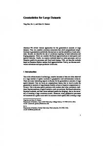
Figure 1 shows the application of the algorithm to a toy data set with arbitrary units generated from the sinc function. The 50 observations have positive exponential noise added. This one-sided noise distribution is highly non-Gaussian, yet the method is able to account for this in learning the posterior Gaussian process. The figure illustrates the loop over the data set in the learning algorithm (steps 2a, 2b ,2c). The posterior distribution is plotted after the algorithm has seen 1, 2, 3, 4, 5, 6, 7, 8, 9, 10, 15, 20, 25, 35 and 50 observations. In each figure only the observations seen so far are plotted. This illustrates how the approximation, which is defined using a maximum of 15 basis vectors, is built sequentially from the observations. In this case a good estimate of the covariance function hyper-parameters is supplied to the algorithm, so there is no need to re-estimate these and recycle the data since a good estimate is obtained after a single pass through the data. While the example is a little contrived, it serves to illustrate our approach. The method is approximate for non-Gaussian noise and non-linear observation operators and thus the order of processing the observations may become important. This can be understood by noting that with non-linear observation operators the log posterior is no longer a quadratic form (Gaussian), rather it may have several local optima, and an unlucky choice of the ordering of the data may result in the algorithm finding such a local minimum. This algorithm is, however, far less sensitive to these type of effects compared to optimisation approaches because the likelihood is integrated (i.e. smoothed) over the prior (see the second term in [9]) and then extremised. To reduce the impact of data ordering on the approximation a data recycling method is introduced that helps minimise the problems of local optima, or poor convergence.

16

3.2

Data recycling

Inference in the online approximation in Csat´o and Opper [2002] is based on a single sweep through the data, but as noted above this might produce a suboptimal approximation to the true posterior. Unfortunately, using further sweeps through the data with the same sequential algorithm in order to achieve a refinement of the approximation would violate the inherent assumption of data independence and would lead to an unprincipled approximation, that is an approximation with no rigorous mathematical justification. The problem of data recycling is overcome using the recently developed expectation propagation framework [Minka 2000]. A principled improvement of the sequential approximation is achieved by altering the Gaussian process posterior, [3], in a way that, although having seen the data once, second and subsequent online inclusions are possible. Intuitively, the effect of the data to be processed is first approximately ‘deleted’ from the solution and only then is included for a second time. When undertaking this deletion it is useful to recall that the projection to the approximating Gaussian process defines a local quadratic approximation to the likelihood for each observation, whose effect is thus easily accounted for and removed. Details of this method can be found in Csat´o [2002], with a more statistical interpretation being given in Cornford, Csat´o, Evans, and Opper [2004].

3.3

Sparsity

The computational complexity of the algorithm remains O(n3 ) if the size of α grows as each observation is sequentially processed. However, the computational cost can be reduced while retaining important information from the data. The parameterisation used for the Gaussian process, q(s(x; α)|Y i , θ, H ), 17

enables the posterior to be written, not in terms of the data, as in the standard geostatistical approaches [4] and [5], but rather in terms of a set of parameters, α, as in the dual kriging equations. These retained α’s are stored at a set of points that we call basis vectors, which can be a subset of the observation locations, but could also be a grid, or the locations at which we want to make predictions. This can be seen in Figure 1) where only a small subset of the observations are used as basis vectors. Estimation of the parameters, α, proceeds sequentially. As each observation is processed (steps 2a, 2b) it is possible to decide at each step whether it is ‘useful’ to increase the number of basis vectors and thus increase the size of α and update these to take account of the observation, as shown in the first two rows of figures in Figure 1). Alternatively, if the new observation does not require a new basis vector the size of α can be left unchanged as in the bottom row of figures in Figure 1). However, it is important to note that the effect of the observation is taken into account through changes to all elements of α. In this way it is possible to restrict the complexity of the algorithm to O(nm2 ), where m is the number of basis vectors retained, and n is the number of observations as before. Alternatively it is possible to specify the minimal loss of information (in the KL-distance sense) that is acceptable, and only add basis vectors where this is exceeded. When approached in this way sparsity ensures a compact representation appropriate to the complexity of the data. Technical details can be found in Csat´o [2002] with a more statistical interpretation in Cornford, Csat´o, Evans, and Opper [2004].

3.4

Hyper-parameter estimation [Figure 2 about here.] 18

Using the sparse Gaussian process framework, it is also possible to perform an approximate estimation of any hyper-parameters in the likelihood or in the Gaussian process covariance functions. The total probability or evidence of the data (the denominator in [3]) given by

p(y | H , θ) =

Z

p(y | s, H )p(s | θ)ds ,

(10)

is maximised with respect to the collection of hyper-parameters. An ‘expectation maximisation’ algorithm for an iterative minimisation of the evidence can be applied. The non-trivial ‘E-Step’ of this algorithm requires the computation of posterior expectations which are approximated consistently using the sparse Gaussian process posterior, q(s(x; α) | Y i , θ, H ), provided by our method Csat´o [2002]. Experiments on highly non-smooth data models such as regression with one sided exponential noise show a rather robust estimation of hyper-parameters with this approach, as exemplified in Figure 2. In Figure 2(a) we have fixed the hyper-parameters to reasonable (but still inappropriate) values and then estimated the posterior with these fixed values, while in (b) the hyper-parameter values are estimated by maximising the evidence after each sweep through the data, resulting in a very good estimate, even though the observations include positive exponential noise. In Figure 2(c) we show that it is possible to learn the hyper-parameters even when the noise model in the likelihood term is not correctly specified. In this case, however the estimate of the posterior distribution of the state is strongly biased, as might be expected. Combining all these steps produces an algorithm that can apply geostatistical modelling methods to problems with very large numbers of observations or non-Gaussian noise models. 19

4

Example application

The sparse Bayesian estimation method is applied to an example one dimensional data set of wave heights. This data set was chosen because the visualisation of the results is easier in the one dimensional setting, and the dataset itself is rather large, with 4096 samples. The example we present is not meant to be an authoritative case study, rather to illustrate the key points of the our sparse, sequential approximation. The data is assumed to have additive Gaussian noise, with a noise variance of 0.04 units2 - the units are actually meters, but this is not important. The initial length scale in the covariance function in the prior is set to 200 units, and the process variance to 0.16 units2 . The mean in the prior is set to zero.

[Figure 3 about here.]

Figure 3 shows an example of applying the sparse sequential algorithm where 2000 samples were used in the estimation, but only 25 basis vectors were retained in the approximation. The data was recycled once through the algorithm prior to hyper-parameters being re-estimated. The hyper-parameters were re-estimated in an outer loop which was performed three times, and a squared exponential covariance functional form was used. The results show that although the use of 25 basis vectors does not allow good fitting of the underlying data, the estimation of the hyper-parameters takes this into account and allows for a larger length scale and process variance which gives a good estimate of the posterior probability distribution, assigning greater uncertainty where the model does not fit the data well.

[Figure 4 about here.] 20

In Figure 4 the method is applied, this time allowing up to 50 basis vectors in the solution, all of which are used. The solution the 50 basis vectors fits the data better than using 25 basis vectors, and the covariance function hyperparameters have been adjusted to reflect this. However, from Figure 4 that more basis vectors would give a better fit to the data.

[Figure 5 about here.]

Figure 5 illustrates the learning algorithm used with up to 200 basis vectors, although only 115 basis vectors are retained in the approximation. This example illustrates the potential of the method, but is not the focus of the paper. An application of the sparse, sequential Bayesian method to inference of a two dimensional, vector posterior Gaussian process, using a variety of non-linear observation operators can be seen in Cornford, Csat´o, Evans, and Opper [2004].

5

Conclusions

This paper shows how a principled, Bayesian approach to geostatistics can be adopted without the need to restrict the application to small problems, or require very long computing times. The algorithm shows that it is possible to develop a Kalman filter like algorithm for simple kriging. The method presented incorporates sparsity and hyper-parameter estimation (variogram modelling) in the same consistent framework. Use of the KL-distance to minimise the discrepancy between the approximating and true posterior provides a principled framework for sparsity and dealing with non-linear H and nonGaussian errors. This allows us to undertake probabilistic inference without 21

having to resort to computationally expensive sampling based methods or applying ad-hoc approximations. As shown in Csat´o [2002] the method can be applied efficiently to binary classification problems through the use of a probit model [Neal 1997], thus could be used within an indicator kriging framework [Cressie 1993]. The method, as implemented, exploits the fact that where we have more observations than are required to fully define the posterior process, the sparse representation in terms of basis vectors is beneficial. This is the case where the sampling density is high with respect to the length scales of the process. Of course the method suffers from several problems, including: • it remains necessary to assume (check) stationarity; • convergence of the algorithm to the global maximum can only be guaranteed in the linear H case – in the non-linear case we can only prove convergence to a fixed point in the learning dynamics. Further empirical work is needed to assess convergence across a range of problems; • interpreting the KL-distances in not trivial – this is not a very intuitive measure for many people; • implementing the method for general observation models, H , requires sampling (low dimensional, but still relatively slow, but no extra coding) or a linearised version of H (generally faster, but may give a worse approximation and requires coding); • at present hyper-parameter estimation is likelihood based, however an extension allowing priors over the hyper-parameters is possible within a maximum a posteriori probability framework; 22

• if the true posterior in [3] is very non-Gaussian, then the Gaussian approximation may be rather poor and thus not particularly useful – this must be judged by the context; • the algorithm involves some quite complex manipulations of the parameters α, and this, together with the use of the expectation propagation method means that it can be rather unstable in cases where the likelihood is very peaked corresponding to a small nugget effect in geostatistics. Most of these drawbacks are either innate to any geostatistical method or are to do with the way the algorithm is implemented. The most serious weakness of the algorithm is that although we can cope with non-linear H , in these circumstances the Gaussian posterior approximation may not be appropriate. This will depend on the problem; if the aim is to infer a nonGaussian posterior then other methods will be required, however is seems that it might well be computationally very efficient to use our approximation as a starting point for efficient population Monte Carlo methods [Capp´e, Guillin, Marin, and Robert ], which could be used to estimate the full non-Gaussian posterior. There is another possibility for sparsity in contrast to the sparsity we exploit. The posterior covariance matrix might itself be sparse, as would arise with covariance models which are space limited, that is have compact support. In this case it would be possible to extend the basis vector sparsity to a sparse representation of the covariance matrix, for instance using an eigendecomposition as in Mardia, Goodall, Redfern, and Alonso [1998, Wikle and Cressie [1999]. This is something we hope to investigate further. We hope to also demonstrate the algorithm on a range of problems and data sets, 23

to assess issues such as hyper-parameter estimation, convergence and data recycling. In future work we hope to look at estimation in Gaussian process mixture models, which will provide a more flexible posterior. It is possible to see the mixture modelling method as being an intermediate complexity solution, where the non-parametric sampling based methods are too slow for practical application. We also plan to extend the model to space-time phenomena with application to data assimilation in numerical weather prediction, but this requires the development of the methodology within a rigorous spacetime framework for stochastic dynamic systems.

Acknowledgements This work was supported by EPSRC grant GR/R61857/01. We are grateful to the conference organisers for inviting submission of this paper, and to the reviewers for their helpful comments and suggestions which have greatly improved the readability of the paper.

References Capp´e, O., A. Guillin, J. Marin, and C. Robert. Population monte carlo. Journal of Computational and Graphical Statistics. (in press). Cornford, D., L. Csat´o, D. J. Evans, and M. Opper 2004. Bayesian analysis of the scatterometer wind retrieval inverse problem: some new approaches. Journal of the Royal Statistical Society B 66, 1–17. Cowles, M. K. and B. P. Carlin 1996. Markov-Chain Monte-Carlo Convergence Diagnostics—A Comparative Review. Journal of the American 24

Statistical Association 91, 883–904. Cressie, N. A. C. 1993. Statistics for Spatial Data. New York: John Wiley and Sons. Csat´o, L. 2002. Gaussian Processes – Iterative Sparse Approximation. Ph.D. thesis, Neural Computing Research Group, Aston Univeristy, http://www.ncrg.aston.ac.uk/Papers. Csat´o, L. and M. Opper 2002. Sparse on-line Gaussian processes. Neural Computation 14, 641–669. Diggle, P. J., J. A. Tawn, and R. A. Moyeed 1998. Model-based geostatistics. Applied Statistics 47, 299–350. Gilks, W., S. Richardson, and D. J. Spiegelhalter 1996. Markov Chain Monte Carlo in Practice. London: Chapman and Hall. Handcock, M. S. and M. L. Stein 1993. A Bayesian analysis of kriging. Technometrics 35, 403–410. Journel, A. G. and C. J. Huijbregts 1978. Mining Geostatistics. London: Academic Press. Mardia, K., C. Goodall, E. Redfern, and F. Alonso 1998. The kriged Kalman filter. Test 7, 217–285. Minka, T. P. 2000. Expectation Propagation for Approximate Bayesian Inference. Ph.D. thesis, Dep. of El. Eng. & Comp. Sci.; MIT, vismod.www.media.mit.edu/∼tpminka. Neal, R. M. 1997. Regression and classification using gaussian process priors (with discussion). In J. M. Bernardo, J. O. Berger, A. P. Dawid, and A. F. M. Smith (Eds.), Bayesian Statistics, Volume 6, pp. 475–501. Oxford: Oxford University Press. 25

Opper, M. and D. Saad (Eds.) 2001. Advanced Mean Field Methods: Theory and Practice. The MIT Press. Press, W. H., S. A. Teukolsky, W. T. Vettering, and B. P. Flannery 1992. Numerical Recipes in C (2nd Edition ed.). Cambridge, UK: Cambridge University Press. Rue, H. and H. Tjelmeland 2002. Fitting Gaussian Markov random fields to Gaussian fields. Scandinavian Journal of Statistics 29, 31–49. Wackernagel, H. 1995. Multivariate Geostatistics. Berlin: Springer-Verlag. Wahba, G. 1991. Spline Models for Observational Data. Philadelphia: Society for Industrial and Applied Mathematics. Wikle, C. K. and N. Cressie 1999. A dimension-reduced approach to spacetime Kalman filtering. Biometrica 86, 815–829.

26

5

5

5

5

5 Signal

10

Signal

10

Signal

10

Signal

10

Signal

10

0

0

0

0

0

−5 −20

−5 −20

−5 −20

−5 −20

−5 −20

−15

−10

−5

0 Distance

5

10

15

20

−15

−10

−5

0 Distance

5

10

15

20

−15

−10

−5

0 Distance

5

10

15

20

−15

−10

−5

0 Distance

5

10

15

20

5

5

5

5

5

0

−5 −20

0

−15

−10

−5

0 Distance

5

10

15

−5 −20

20

0

−15

−10

−5

0 Distance

5

10

15

−5 −20

20

0

−15

−10

−5

0 Distance

5

10

15

−5 −20

20

−15

−10

−5

0 Distance

5

10

15

−5 −20

20

5

5

5

5

0

0

0

0

0

−5 −20

−5 −20

−5 −20

−5 −20

−5 −20

−5

0 Distance

5

10

15

20

−15

−10

−5

0 Distance

5

10

15

20

−15

−10

−5

0 Distance

5

10

15

20

−5

0 Distance

5

10

15

20

−15

−10

−5

0 Distance

5

10

15

20

−15

−10

−5

0 Distance

5

10

15

20

Signal

5

Signal

10

Signal

10

Signal

10

Signal

10

−10

−10

0

10

−15

−15

Signal

10

Signal

10

Signal

10

Signal

10

Signal

10

−15

−10

−5

0 Distance

5

10

15

20

Figure 1: An example showing how the method is able to sequentially estimate the posterior distribution of the state (mean given by the solid black line, +/- one standard deviation given by the grey lines line, plotted in state space, not observation space), given observations (grey dots) with very nonGaussian (single sided exponential) noise. The true generating process is given by the solid thick grey line, and the basis vectors are given by the circled crosses. The top left figure shows the posterior distribution after one observation has been seen. The subsequent figures (right, then down) show the posterior distribution after 2, 3, 4, 5, 6, 7, 8, 9, 10, 15, 20, 25, 35 and 50 observations have been seen.

27

10

10

8

12

10

8

6

8

Signal

Signal

Signal

6 4

4

2

6

4 2

0

2 0

−2

−4 −20

−15

−10

−5

0 Distance

5

10

15

20

−2 −20

0

−15

−10

−5

(a)

0 Distance

(b)

5

10

15

20

−2 −20

−15

−10

−5

0 Distance

5

10

15

(c)

Figure 2: The same example set up as in Figure 1 with one sided exponential noise. In (a) the hyper-parameters are fixed, while in (b) they are estimated from the data using our algorithm. In (c) the effect of using an incorrect noise model in the likelihood is shown.

28

20

0.8 0.6

Wave height

0.4 0.2 0 −0.2 −0.4 −0.6 −0.8 0

500

1000

1500

2000 Distance

2500

3000

3500

4000

Figure 3: An example of the estimation of the posterior processes on a data set consisting of a series of wave height measurements permitting a maximum of 25 basis vectors. The plot shows the training points (light grey dots), the basis vectors (black circled crosses), the posterior mean of the Gaussian process (dark solid line) and the posterior variance (plotted at plus / minus one standard deviation, the grey lines).

29

0.8 0.6

Wave height

0.4 0.2 0 −0.2 −0.4 −0.6 −0.8 0

500

1000

1500

2000 Distance

2500

3000

3500

Figure 4: Similar plot to Figure 3 with 50 basis vectors in the solution.

30

4000

0.8 0.6

Wave height

0.4 0.2 0 −0.2 −0.4 −0.6 −0.8 0

500

1000

1500

2000 Distance

2500

3000

3500

4000

Figure 5: Similar plot to Figure 3, but permitting up to 200 basis vectors in the solution.

31