Sequential clustering with particle filters − Estimating the number of clusters from data Johan Schubert Department of Data and Information Fusion Division of Command and Control Systems Swedish Defence Research Agency SE-164 90 Stockholm, Sweden
[email protected] http://www.foi.se/fusion/ Abstract - In this paper we develop a particle filtering approach for grouping observations into an unspecified number of clusters. Each cluster corresponds to a potential target from which the observations originate. A potential clustering with a specified number of clusters is represented by an association hypothesis. Whenever a new report arrives, a posterior distribution over all hypotheses is iteratively calculated from a prior distribution, an update model and a likelihood function. The update model is based on an association probability for clusters given the probability of false detection and a derived probability of an unobserved target. The likelihood of each hypothesis is derived from a cost value of associating the current report with its corresponding cluster according to the hypothesis. A set of hypotheses is maintained by Monte Carlo sampling. In this case, the state-space, i.e., the space of all hypotheses, is discrete with a linearly growing dimensionality over time. To lower the complexity further, hypotheses are combined if their clusters are close to each other in the observation space. Finally, for each time-step, the posterior distribution is projected into a distribution over the number of clusters. Compared to earlier information theoretic approaches for finding the number of clusters this approach does not require a large number of trial clusterings, since it maintains an estimate of the number of clusters along with the cluster configuration. Keywords: Particle filtering, sequential Monte Carlo, clustering, finding the number of clusters.
1 Introduction In this paper we develop a particle filtering approach for grouping target observation reports into an unspecified number of clusters. We let each cluster correspond to one of the potential targets from which the observations originates. This method solves exactly the same problem as the one by Schubert [1] and Bengtsson and Schubert [2] except that it handles the reports sequentially and does not need to be given the number of clusters. Thus, given a large number of reports of target observations arriving sequentially, it determines the number of targets and associates each report with a target. Basically, this is a Bayesian filter in which the statespace grows in each step when receiving a report. It can also be thought of as a “soft” decision tree with pruning. The state-space is then simply all possible association hypotheses. It is discrete and one-dimensional.
0-7803-9286-8/05/$20.00 © 2005 IEEE
Hedvig Sidenbladh Department of IR Systems Division of Sensor Technology Swedish Defence Research Agency SE-164 90 Stockholm, Sweden
[email protected]
[]
Report 1
Report 2
[0]
[0,0]
[0,1]
[1]
[1,0]
[1,1]
[1,2]
etc. Fig. 1. Illustration of the growth of the state-space over filter steps. Note that the numbers of the clusters are not necessarily the same in different subtrees. The number does not reflect the identity of the cluster. Instead, clusters are given numbers in a specific hypothesis based on how many previous clusters there are according to this hypothesis. The largest number in the hypothesis reflects the number of clusters. Cluster number “0” means that this report is regarded as clutter and not associated with a cluster.
In Fig. 1 the structure of the state-space is visualized. At the arrival of the first report, the state-space has only two states, [0] and [1]. We let the value “0” mean clutter, and let the value “1” mean a target given a target number of “1”. Obviously, if the first report is in state [0] it means the report was due to clutter, and if it is in state [1] it means that the report originated from the target at hand (with target number “1”). Thus, the state of each report corresponds to a hypothesis about the report to target (track) association. When a second report arrives, the discrete state-space grows to five possible states, Fig. 1. Each state at the first level leads to two or three different states at the second level (see Section 3.1). At this time [0] and [1] are no longer part of the state-space. The state-space will now only consist of the five elements of length two in the bottom row of Fig. 1. Thus, the elements of the state-space are always of the same length, where each element is an
alternative hypothesis about the target association of all observations. For example, the state [0, 1] means that the first report was clutter, while the second report originates from a target with target number “1”. We may also conclude that there is one target according to this state, since “1” is the highest target number of the state. With three reports there are 15 possible states, and with four report 52 possible states, etc.1 Since the number of possible states grows somewhat faster than simple exponentially, we must perform some hard pruning. When we receive a new report, a posterior distribution over all hypotheses is iteratively calculated from a prior distribution using an update model and a likelihood function. The update model updates the probability of all active hypotheses from a previous time-step k − 1 to the current time-step k. Given the prior distribution, the probabilities of all current hypotheses are updated through the update model which is based on an association probability for clusters given the probability of false detection and a derived probability of an unobserved target. False detection and detection of a new previously unobserved target are handled as two important special cases. The likelihood of each maintained hypothesis is derived from a cost value of associating the current report with its corresponding cluster. We will assume a likelihood for each hypothesis that declines with the distance, Eq. (7), between the new report and the cluster center. The set of active hypotheses is maintained by Monte Carlo sampling [3, 4] as in an ordinary particle filter [5], [6]. At each time-step, we will only propagate those states which have posterior probability higher than a certain threshold. All other states are assigned zero probability and are eliminated. This is achieved indirectly by using a fixed number of particles. Whatever remains are the active hypotheses maintained in the analysis. As many states with a small likelihood are not sampled with the Monte Carlo algorithm we avoid a combinatorial explosion. On the other hand, some states are sampled several times, then we record the number of particles at that state by a variable and adjust the probability accordingly, rather than keep several identical copies. In order to lower the computational complexity, we will also combine any hypotheses with equal number of clusters if their clusters are close enough to each other in the observation space. Apart from the actual clustering of observations, one of the major issues of importance is the estimated number of clusters. This is estimated by projecting the obtained posterior distribution into a distribution over the number of clusters. As far as we know, this is the first paper using particle filtering for finding the number of clusters. The intended application is for an intelligence preprocessor method in any multi-target environment where the number of targets are unknown and observation to target association has to be performed before other fusion methods can be applied, e.g., as in [7, 8].
11,
2, 5, 15, 52, 203, 877, 4140, 21147, 115975, 678570, ...
In Section 2 we discuss the cluster problem and why the methodology developed in this paper is needed. In Section 3 we develop a general algorithm for determining the number of clusters from an incoming stream of reports and discuss its worst case computational complexity. In Sections 4 and 5 we describe a metric and a conflict based distance measure between reports, respectively. In Section 6 we discuss parameter settings and performance on time complexity, convergence and quality of results. Finally, in Section 7, conclusions are drawn.
2 Clustering When receiving a large number of observations in an environment with several targets where observations are not pre-associated with targets, we need to have some association or clustering method [9, 10] to perform an association before we can proceed. When using a cluster method it is usually necessary to know up-front the actual number of clusters as this is an input parameter in most clustering methods. When no knowledge of the true number of clusters is available we must estimate this from data as is done in this paper or run several different trial clusterings, with different fixed number of clusters, as was done in Ahlberg et al. [7] and Schubert et al. [8] with Dempster-Shafer [11, 12] cluster using Potts mean filed theory [2, 13−17]. We could then estimate the number of clusters from the rate of change in conflict between trials with different number of clusters using, e.g., the L method [18]. If some apriori information is available, such as a probability distribution over the number of clusters such information can be used directly in the clustering process, as was done in [19]. This would render an approach as in this paper unnecessary. However, in the general case when no a priori information regarding the number of clusters is available we must infer the actual number of clusters from data. While it is possible to estimate the number of clusters directly from all data without clustering using only detection probability, the enormous number of alternative association hypotheses must be reduced by eliminating low probability hypotheses, otherwise the problem will be intractable computationally. An organized approach to manage hypotheses is to receive observations sequentially and eliminate low probability hypotheses as we go. This approach obviously fits well with any problem that is sequential in nature.
3 Bayesian Sequential Clustering Each element of the state-space in which the filtering takes place is a vector of numbers, indicating the cluster identities of each observed report (Fig. 1). Let the stochastic variable Xk = [I1, ..., Ik] denote the state at step k, and xk = [i1, ..., ik] a certain value of Xk, i.e., a certain state. Thus, at step k we have received k observations and all elements of the state-space xk are of length k, where ik is a target number of an observation zk according to hypothesis xk. Each element of the state-space is an alternative hypothesis about the observation-to-target
association of all observations received. The number of objects according to the hypothesis xk can be obtained as nk = max(xk) = max([i1, ..., ik]). Furthermore, let the stochastic variable Zk be the report at step k, and zk a certain value of Zk, i.e., the observed report. The result of the filter in each step is the discrete posterior distribution over association hypotheses given the history of reports z1:k. From this distribution we can obtain the MAP estimate, i.e., the most probable hypothesis so far. By taking the marginal of the distribution with respect to object count, we can also obtain a distribution over the number of objects Nk, p N z (n k z 1:k ) . The posterior is iteratively obtained from k 1:k the previous step as: P(X k = x k Z 1:k = z 1:k ) = p x pz
k
x k (z k
xk) ∑ px xk – 1
px
k
k
z 1:k (x k
x k – 1(x k
k–1
z 1:k ) ∝
x k – 1)
z 1:k – 1(x k – 1
(1) z 1:k – 1)
where p z px k px
(z k x k ) is the likelihood of hypothesis xk, k xk ( x x is the update model and x k – 1 k k – 1) ( x z ) the posterior at the previous step. z k – 1 1:k – 1
k–1
1:k – 1
3.1 Update The update step derives a prior distribution at step k from the posterior distribution at step k − 1, given the update model p x x (x k x k – 1) . The state xk is a concatenation of k k–1 xk − 1 and the target number ik to which report zk is associated in this hypothesis: xk = [xk − 1, ik]. The distribution over xk consists of two special cases and a general case. 3.1.1 Special case 1: Clutter. If ik is set to “0”, the report zk is assumed to be clutter, and not associated with any cluster. The probability of this, pFP , is known and depends on the sensor. Thus px
k
x k – 1([ x k – 1,
0 ] x k – 1) = p FP .
(2)
3.1.2 Special case 2: New cluster. If ik is set to max(xk − 1) + 1, a previously un-observed target is hypothesized. This is equivalent to assuming that a fraction 1 1 ----- = -----------------------------------max(x k – 1) + 1 nk
(3)
of the observations 1 to k − 1 were clutter, given that all targets have equal probability of being observed. The probability of this is p B = p PF
k–1 ----------nk .
px
k
x k – 1([ x k – 1,
n k ] x k – 1) = p B ( 1 – p FP ) .
(5)
3.1.3 General case: Report associated with existing cluster. The prior for 1 ≤ i k ≤ max(x k – 1) is px
k
x k – 1([ x k – 1, i k ]
( 1 – p B ) ( 1 – p FP ) x k – 1) = --------------------------------------------max(x k – 1)
(6)
given that all targets have equal probability of being observed.
3.2 Observation The observation likelihood p z x (z k x k ) states the k k probability of observing report zk given association hypothesis xk. It is dependent on differences between reports referring to the same target (according to hypothesis xk). In our test example, presented further in Section 5, the objects generating the observations are static, and live on a two-dimensional surface. Observations are noisy versions of the 2D object position. Denote the number of clusters according to hypothesis xk, nk. From xk, nk cluster means [ M 1, …, M n ] can be computed, as the Euclidean mean k position of all observations clustered in the same cluster. These cluster means are the estimated positions of the nk objects that generated the observations [ z 1, …, z k ] . According to hypothesis x k = [ i 1, …, i k ] , the observation zk has been generated from object ik. Assuming Gaussian observation noise with standard deviation σ, the likelihood is 2
pz
k
x k (z k
xk) ∝
zk – Mi k – -------------------------2σ 2 e
(7)
if ik > 0. When ik = 0 the likelihood is uniformly distributed over the 2D observation space.
4 Particle Filter Implementation The Bayesian sequential clustering algorithm is implemented as a particle filter. The posterior distribution over Xk is represented by a set of N state hypotheses, or particles { ξ 1k , …, ξ Nk } . The number of particles at a certain position in the discrete state-space represents the posterior density in that point [5, 20]. In reality, the particles at position number h in the (discrete) state-space is represented by a tuple ( x hk , π hk ) where x hk is the state and π hk is proportional to the number of particles at that state. The number of such hypotheses, N hk , is most often several orders of magnitude smaller than N . The choice of N is discussed further in Section 5. Fig. 2 gives an overview of the algorithm.
4.1 Update (4)
This leads to the probability of a new, previously unobserved cluster,
From each old hypothesis ( x hk – 1, π hk – 1 ) , n hk – 1 + 2 new prior hypotheses ( x hk , π˜ hk ) are instantiated, one for each of the two special cases, and one each for the n hk – 1 clusters according to hypothesis x hk – 1 (see Section 3.1, Fig. 3).
d (h 1, h 2) =
% propagate: h for h ← 1: N k – 1
% from previous step: h
h
% posterior ( x k – 1, π k – 1 ) . h
for h ← 1: n k – 1 + 2 compute each possible prior h probability π˜ k , from
fx
compute likelihood ϖ hk
← π˜ hk f z
k
x hk , and its h h (x k x k – 1) . k
x k (z k
x hk )
.
end
% normalize, resample: h h
normalize weight ϖ k ←
ϖ hk
∑ ------i . i
end
(8)
xk – 1
end
for h ← 1: N k
h h ∞, nk 1 ≠ nk 2 . max M h1 – M h2 , …, M h1 – M h 2 1 k k 1 h2 h1 ----------------------------------------------------------------------------------------------- , n k = n k σ
ϖk
For all pairs of hypotheses h1, h2, we compute d(h1, h2). If the measure is smaller than 1, i.e., within one standard deviation, the hypothesis with the lowest weight is removed, and the weight of the other hypothesis is set to h h πk 1 + πk 2 . This lowers the number of hypotheses when the variance in the set of hypotheses is low, i.e., when the clustering algorithm is “sure” about the right solution (see Section 5, Fig. 4a).
for i ← N j
monte carlo sample posterior ξ k from Nh Nh 1 weighted set { ( x k , ϖ 1k ), …, x k k, ϖ k )} . k
end 1
1
Nh
4.5 State Estimation The cluster result at step k can be defined as the maximum a posteriori (MAP) estimate
Nh
Derive weighted set { ( x k , ϖ k ), …, ( x k k, ϖ k k )} from 1 N particle set { ξ k , …, ξ k } .
Fig. 2. Pseudo code for step k in a clustering particle filter.
The new prior weights π˜ hk = π hk – 1 p x x (x hk x hk – 1) are k k–1 calculated according to Eqs. (2, 5, 6). The new h ˜h hypotheses ( x k , π k ) constitute the prior distribution at step k.
4.2 Observation The likelihood of each hypothesis x hk is computed according to Eq. (7). The hypotheses ( x hk , ϖ hk ) , where h ϖ hk = π˜ hk p z x (z k x k ) , represent the posterior distribution k k over cluster hypotheses at step k.
4.3 Resampling Now N particles { ξ 1k , …, ξ Nk } are Monte Carlo sampled from the discrete distribution ( x hk , ϖ hk ) . As described above, the particles are represented by N hk states, and the number of particles at that state, ( x hk , π hk ) . The states ( x hk , π hk ) also represent the posterior distribution over cluster hypotheses at step k. However, the new number of states N hk is much smaller than N hk , in that many states x hk with a small likelihood ϖ hk were not drawn during the sampling. Due to the resampling with a constant number N particles, the number of hypotheses N hk do not grow with k, as we shall see in Section 5.
4.4 Collapsing Hypotheses When the observation space is metric, one can define a measure d of hypothesis similarity. Here, this measure is defined as
arg max h(π hk )
x MAP = xk k
.
(9)
The estimated number of clusters at step k can be estimated as the expected a posteriori (EAP) estimate
= n EAP k
πh h k ----n ∑ k N. h
(10)
5 Experiments The clustering method was implemented in MATLAB and carried out on a desktop PC with a 2 GHz Pentium III processor. For testing, a 2D static scenario was generated. A selected number of n objects xi = [xi, x, xi, y] were randomly placed on a 10 × 10 square. Observations were generated from this scene. With probability pFP = 0.2, the observations zk = [zk, x, xk, y] were sampled from a uniform distribution U([0, 0], [10, 10]) over the square. With probability 1 − pFP = 0.8, the observations were sampled from a Gaussian distribution G(xi, σ), i ∈ [1, n] around any of the objects. The standard deviation of observations was set to σ = 0.2.
5.1 Computational Complexity An interesting feature of the algorithm is its computational complexity, convergence time and performance with respect to the number of objects n in the scenario. Fig. 3a,b show that the maximum number of hypotheses N hk increases as O(en). Likewise, the CPU time required to find a solution, T, increases as O(en). This is further discussed in Section 6.
Max number of hypotheses 9
8
8
log(number of hypotheses)
log(number of hypotheses)
Max number of hypotheses 9
7
6
5
4
3
4
5
6
7
8
7
6
5
4
3
9
4
5
Number of objects
(a) The logarithm of the maximum number of hypotheses, N hk , as a function of the number of objects n. Exponentially growing N . N hk grows as O (en).
8
8
7
7
6
6
5 4 3
4 3 2
1
1
6
7
8
0
9
4
5
Number of objects
0.9
0.9
0.8
0.8
0.7
0.7
0.6 0.5
0.5 0.4
0.3
0.3
7
9
0.6
0.4
6
8
P(correct) at step 3*(number of objects) 1
P(correct)
P(correct)
P(correct) at step 3*(number of objects)
5
7
(d) The logarithm of the CPU time required for the classifier to reach a 90% certainty about the correct number of objects n, as a function of the number of objects n. Constant N . The computation time starts at a higher value, and grows as O (en), but with a lower constant.
1
4
6
Number of objects
(c) The logarithm of the CPU time T required for the classifier to reach a 90% certainty about the correct number of objects n, as a function of the number of objects n. Exponentially growing N . The computation time grows as O (en).
0.2
9
5
2
5
8
CPU time to P(number of objects) = 90% 9
log(CPU time)
log(CPU time)
CPU time to P(number of objects) = 90%
4
7
(b) The logarithm of the maximum number of hypotheses N hk , as a function of the number of objects n. Constant N . N hk starts at a higher value, and grows as O (en), but with a lower constant.
9
0
6
Number of objects
8
9
Number of objects
(e) The probability of correct number of objects n after 3n observations have arrived, as a function of the number of objects n. Exponentially growing N .
0.2
4
5
6
7
8
9
Number of objects
(f) The probability of correct number of objects n after 3n observations have arrived, as a function of the number of objects n. Constant N .
Fig. 3. Complexity experiment. For each number of objects n, the clustering was carried out five times. The values in the graphs above are the medians of values extracted from these five runs.
5.1.1 Choosing the number of particles.
Estimated number of clusters 10
We tested two approaches, to use an exponentially growing number of particles N n = 600 . 1.6n, n = 4, ..., 9, and a constant number of particles N = N 9. Fig. 3a,c,e show the statistics using the exponentially growing number of particles, while Fig. 3b,d,f show the statistics using a constant number of particles. The exponential growth in computation time with respect to n (Fig. 3c) is not entirely due to the exponentially growing number of particles − Fig. 3d also shows an exponentially increasing computation time.
5 0
0
50 100 Marginal posterior probability of the true number of clusters
150
0
50 100 Number of hypotheses
150
0
50 100 Computation time per observation [s]
150
1 0.5 0 4000 2000 0 40
5.2 Comparison with Other Method The method was compared to another, non-sequential, clustering method, i.e., Potts spin clustering [2]. While Fig. 4a,b show the performance and result of our sequential method on a n = 8 object problem, Fig. 4c shows the result of the Potts spin method. The Potts spin method requires knowledge of the actual number of clusters, while the method developed in this paper determines the number of clusters directly from data. The clustering result is virtually the same, with the exception that our method classifies outlier observations as not part of any cluster, while the Potts spin method puts each observation into some cluster. The Potts spin clustering method required a CPU time of 1.02 s for one clustering process with 150 observations clustered into eight clusters, while the sequential clustering method developed in this paper required an average of 11.57 s for each of 150 sequential associations between an observation and one to ten clusters, Fig. 4a. The total CPU time for this was 1736 s. However, when the number of objects is unknown a separate Potts spin clustering has to be performed for each hypothesis about the number of objects − in a trial application we performed 21 clusterings for different number of clusters at each time-step [8]. Furthermore, if the clustering has to be performed sequentially, a new clustering has to be made for each new arriving observation, in this case 150 times. Thus, the Potts spin clustering has to be performed 3150 times in order to achieve the same full functionality as with sequential clustering. This would take approximately twice the computation time compared to the sequential approach. The method developed in this paper is only suitable with sequential mid sized problems (with respect to number of clusters) when the number of clusters is unknown − in other situations, a non-sequential clustering method is preferred. It should be noted that the method can handle large amounts of data (as long as the number of clusters is not growing) without computational problems since it has a linear time complexity in the number of observations.
6 Discussion The behavior of the sequential clustering algorithm is controlled by just two parameters, the false detection probability pFP and the number of particles N , and one
20 0
0
50
100
150
(a) Statistics from a clustering of observations with n = 8. 10 9 8 7 6 5 4 3 2 1 0
0
2
4
6
8
10
(b) The best hypothesis at the last step of this clustering. 10 9 8 7 6 5 4 3 2 1 0
0
2
4
6
8
10
(c) A Potts spin clustering using the same set of observations, with the correct number of objects as an input parameter. Fig. 4. Comparison with another clustering method. Both clusterings used the same set of observations. The number of objects in the simulation was n = 8.
measure d of hypothesis similarity determining when collapsing two hypotheses into one. From the detection probability we derive the probability of a new cluster and the probability of association with existing clusters. This model simplicity makes it very simple to adjust the algorithm for different applications. The experiment carried out has the same simplicity. It is characterized by the standard deviation σ of a Gaussian distribution around targets. The likelihood of the algorithm is dependent on the standard deviation and thus controlled by the experiment. In these experiments we chose a false detection probability of 0.2 and a standard deviation of 0.2. Together with the random target distribution the resulting set of observations and their clustering can be viewed in Fig. 4b. Obviously, the target distribution is rather sparse relative to the standard deviation and result must be viewed in that light. However, our main interest is to compare the quality of the clustering and performance of the sequential algorithm relative an existing non-sequential method. The convergence of the sequential algorithm is quite good. After receiving roughly four observations per cluster the probability of the correct number of clusters is higher than 50%, after seven observations it is about 90%. Given the very high pruning of hypotheses made by particle filtering in keeping a fixed number of particles, this seems quite satisfactory. After looking carefully at Fig. 4b, the same thing can be said about quality of results. In spite of the high pruning of low probability hypotheses there are only some very few observations close to cluster centers that seem misclassified as clutter. No true clutter seem to be misclassified as genuine observations. This result is almost as good as that of Potts spin, Fig. 4c. One advantage of the sequential Monte Carlo algorithm compared to Potts spin is its ability to classify clutter as such. This is ignored in the standard implementation of Potts spin clustering. Finally, a computational complexity of O( k e nk ), i.e., exponential in the number of clusters makes the sequential Monte Carlo method unsuitable for large scale problems. Potts spin with a polynomial computational complexity in the number of clusters of O( k 2 n k2 ) can manage much larger problems. With respect to number of observations though, the sequential algorithm has a linear computation complexity, while Potts spin is again polynomial.
7 Conclusions In this paper we have developed a sequential clustering approach with particle filtering that makes it possible to cluster observations into a unknown number of clusters. The quality of associations made is virtually equal to a previous non-sequential method that was fed the actual number of clusters. As the method has a linear time complexity in the number of observations, but an exponential time complexity in the number of clusters it is only suitable for mid sized problems (with respect to number of clusters), but can handle large amounts of observations. This is both
an advantage and a draw-back compared to the nonsequential method. Obviously, the method fits especially well with problems that are sequential in nature, when computation time for each update is more important than total computation time.
Acknowledgments Thanks to Neil Gordon and Alan Marrs for suggesting using particle filters for clustering.
References [1] Johan Schubert. On nonspecific evidence. International Journal of Intelligent System, 8(6):711−725, 1993. [2] Mats Bengtsson and Johan Schubert. Dempster-Shafer clustering using potts spin mean field theory. Soft Computing, 5(3):215−228, 2001. [3] Marshall N. Rosenbluth and Arianna W. Rosenbluth. Monte Carlo calculation of the average extension of molecular chains. The Journal of Chemical Physics, 23(2):356−359, 1955. [4] Jun S. Liu. Monte Carlo strategies in scientific computing. Springer-Verlag, New York, NY, 2001. [5] Neil J. Gordon, David J. Salmond, and Adrian F.M. Smith. Novel approach to nonlinear/non-Gaussian Bayesian state estimation. IEE Proceedings F (Radar and Signal Processing), 140(2):107−113, 1993. [6] Arnaud Doucet, Nando de Freitas, and Neil J. Gordon. Sequential Monte Carlo Methods in Practice, SpringerVerlag, New York, NY, 2001. [7] Simon Ahlberg, Pontus Hörling, Karsten Jöred, Christian Mårtenson, Göran Neider, Johan Schubert, Hedvig Sidenbladh, Pontus Svenson, Per Svensson, Katarina Undén, and Johan Walter. The IFD03 information fusion demonstrator. In Per Svensson and Johan Schubert, editors, Proceedings of the Seventh International Conference on Information Fusion, volume II, pages 936−943, Stockholm, Sweden, 28 June−1 July 2004. International Society of Information Fusion, Mountain View, CA, 2004. [8] Johan Schubert, Christian Mårtenson, Hedvig Sidenbladh, Pontus Svenson, and Johan Walter. Methods and system design of the IFD03 information fusion demonstrator. In Cd Proceedings of the Ninth International Command and Control Research and Technology Symposium, track 7.2, paper 061, pages 1−29, Copenhagen, Denmark, 14−16 September 2004. US Department of Defence CCRP, Washington, DC, 2004. [9] Anil K. Jain and Richard C. Dubes. Algorithms for Clustering Data, Prentice-Hall, Englewood Cliffs, NJ, 1988. [10] Anil K. Jain, M. Narasimha Murty, and Patrick J. Flynn. Data clustering: a review, ACM Computing Surveys, 31(3):264−323, 1999. [11] Arthur P. Dempster. A generalization of Bayesian inference. Journal of the Royal Statistical Society (Series B), 30(2):205−247, 1968. [12] Glenn Shafer. A mathematical theory of evidence, Princeton University Press, Princeton, NJ, 1976.
[13] Johan Schubert. Clustering belief functions based on attracting and conflicting metalevel evidence using Potts spin mean field theory. Information Fusion, 5(4):309−318, 2004. [14] Johan Schubert. Clustering belief functions based on attracting and conflicting metalevel evidence. In Bernadette Bouchon-Meunier, Laurent Foulloy, and Ronald R. Yager, editors, Intelligent Systems for Information Processing: From Representation to Applications, pages 349−360, Elsevier Science, Amsterdam, 2003. [15] Carsten Peterson and Bo Söderberg. A new method for mapping optimization problems onto neural networks. International Journal of Neural Systems, 1(1):3−22, 1989. [16] Renfrey B. Potts. Some generalized order-disorder transformations. Proceedings of the Cambridge Philosophical Society, 48:106−109, 1952.
[17] Fred Y. Wu. The Potts model. Reviews of Modern Physics, 54(1):235−268, 1982. [18] Stan Salvador and Philip Chan. Determining the Number of Clusters/Segments in Hierarchical Clustering/Segmentation Algorithms. Technical Report CS-2003-05, Department of Computer Sciences, Florida Institute of Technology, Melbourne, FL, 2003. [19] Johan Schubert. Simultaneous Dempster-Shafer clustering and gradual determination of number of clusters using a neural network structure. In Proceedings of the 1999 Information, Decision and Control Conference, pages 401− 406, Adelaide, Australia, 8−10 February 1999. IEEE, Piscataway, NJ, 1999. [20] Michael Isard and Andrew Blake. Condensation − conditional density propagation for visual tracking. International Journal of Computer Vision, 29(1):5−28, 1998.