Sequential Conformal Anomaly Detection in Trajectories based on ...

14th International Conference on Information Fusion Chicago, Illinois, USA, July 5-8, 2011

Sequential Conformal Anomaly Detection in Trajectories based on Hausdorff Distance Rikard Laxhammar∗† and G¨oran Falkman∗ Research Centre, University of Sk¨ovde, Sk¨ovde, Sweden † Security and Defense Solutions, Saab AB, J¨ arf¨alla, Sweden {rikard.laxhammar, goran.falkman}@his.se

∗ Informatics

Abstract—Abnormal behaviour may indicate important objects and situations in e.g. surveillance applications. This paper is concerned with algorithms for automated anomaly detection in trajectory data. Based on the theory of Conformal prediction, we propose the Similarity based Nearest Neighbour Conformal Anomaly Detector (SNN-CAD) which is a parameter-light algorithm for on-line learning and anomaly detection with wellcalibrated false alarm rate. The only design parameter in SNNCAD is the dissimilarity measure. We propose two parameterfree dissimilarity measures based on Hausdorff distance for comparing multi-dimensional trajectories of arbitrary length. One of these measures is appropriate for sequential anomaly detection in incomplete trajectories. The proposed algorithms are evaluated using two public data sets. Results show that high sensitivity to labelled anomalies and low false alarm rate can be achieved without any parameter tuning.

our work, we adopt the statistical definition of an outlier given by Hawkins: “[an outlier is] an observation that deviates so much from other observations as to arouse suspicion that it was generated by a different mechanism” [2]. The mechanism of the other observations is usually assumed to follow a stationary probability distribution. Hence, outlier detection involves determining whether or not a particular observation has been generated by the same distribution as a set of reference observations. Translating this to anomaly detection is straightforward: an anomaly corresponds to an outlier and training data correspond to the reference set.

Keywords: Anomaly detection, trajectory data, Conformal prediction, Hausdorff distance, automated surveillance.

A significant amount of work related to automated anomaly detection in trajectory data has been published in the video surveillance domain [3]. Most of these methods are based on unsupervised trajectory clustering algorithms where trajectories are assigned an anomaly score proportional to the distance to the nearest cluster. In case of probabilistic models, distance is usually expressed in terms of the trajectory likelihood. A central problem is how trajectories should be represented, i.e. what features should be extracted, and how similarity between trajectories should be calculated. The Euclidean distance is perhaps the simplest and most intuitive distance measure, but requires that trajectories are properly aligned and of equal length. Various pre-processing methods and modifications of the Euclidean distance, e.g. Dynamic Time Warping, have been proposed for relaxing alignment constraints [3]. Other approaches reduce trajectories to a fixed low-dimensional representation using various transforms [4]. Abstract and hierarchical representations have also been proposed where trajectories are composed of a number of basic movement patterns, such as Motifs [5]. Many of the proposed algorithms are essentially designed for anomaly detection in complete trajectories, i.e. all data points from the trajectory are required before classifying it as anomalous or not. This is obviously a limitation in surveillance applications since it delays anomaly alarms and thus the ability to react to impending events. In contrast, algorithms for sequential (also known as on-line) trajectory anomaly detection allow detection in incomplete trajectories. Examples of such algorithms have been proposed for video surveillance [3], [6] and maritime surveillance [7], [8] where a probabilistic model is estimated for the momentary location

I. I NTRODUCTION Anomaly detection is an important technique for detecting critical events in a wide range of data rich domains where a majority of the data is considered “normal” and uninteresting. One such domain is surveillance where there is a clear trend towards more and more advanced sensor systems producing huge amounts of trajectory data from moving objects, such as people, vehicles, vessels and animals. In the maritime domain, for example, abnormal behaviour, such as unexpected stops, deviations from standard routes and traffic direction violations, may indicate threats and dangers related to e.g. smuggling, sea drunkenness or accidents. Timely detection of these anomalies is critical for enabling pro-active measures. However, it is clear that accurate and reliable analysis of all trajectories constitutes a great, if not impossible, challenge to human analysts. Thus, there is a need for automated trajectory analysis. This paper is concerned with data-driven algorithms for automated anomaly detection in trajectory data. The main contribution is the proposal and evaluation of a novel and parameter-light algorithm for on-line learning and sequential anomaly detection in trajectory data. But before we discuss previous work and issues related to this topic, let us define what we mean by anomaly detection. There exist multiple yet similar definitions of anomaly detection and the closely related concepts outlier detection and novelty detection (see e.g. [1]). Most of the definitions are based on the idea that anomalies are deviations from a normalcy model which can be learnt from training data. In

978-0-9824438-3-5 ©2011 ISIF

A. Anomaly detection in trajectory data

153

and velocity vector of trajectories. In some cases, anomaly scores for individual data points are integrated within a sliding window [8], [6]; however, these methods are limited, since the feature model is point-based and thus do not capture trajectory behaviour over time. With a few exceptions, learning in previous algorithms is off-line: fixed model parameters and thresholds are typically estimated or tuned once based on a batch of historical data. The need for on-line learning based on new training data has been identified by Piciarelli et al. who proposed an online trajectory clustering algorithm [9]. On-line learning is an important property in the surveillance domain since it enables continuous adaption to new and previously unseen normal behaviour. B. Parameter-laden Algorithms and the Problem of Tuning Thresholds Most anomaly detection algorithms require careful setting of multiple application specific parameters in order to achieve (near) optimal performance. In fact, Keogh et al. argue that most data mining algorithms are more or less parameter-laden, which is undesirable for several reasons [10]. According to Markou and Singh, “an [anomaly] detection method should aim to minimise the number of parameters that are user set” [11]. One could argue that the use of few parameters suppresses bias towards particular types of anomalies and makes the method easier to implement for different applications. The anomaly threshold is a central parameter since it regulates the sensitivity to true anomalies and the false alarm rate (rate of false anomalies). According to Axelsson, “the false alarm rate is the limiting factor for the performance of [an anomaly] detection system” [12]. Hence, maintaining a low and well-calibrated false alarm rate is an important issue. Many algorithms rely on a distance or density threshold for deciding whether new data is anomalous or not [1]. But the distances or densities are typically not normalised and the procedures for setting the thresholds seem to be rather ad-hoc and not intuitive to operators of surveillance systems. C. Contributions of this paper In this paper, we introduce the Similarity based Nearest Neighbour Conformal Anomaly Detector (SNN-CAD) which is a parameter-light algorithm for on-line learning and automated anomaly detection. SNN-CAD is based on the theory of Conformal prediction [13] and a key property that follows from this is that the false alarm rate is well-calibrated; if training data and new normal data are independent and identically distributed (IID), the expected false alarm rate is equal to the specified anomaly threshold  ∈ (0, 1). Thus, in contrast to previously proposed algorithms, SNN-CAD does not require any application specific anomaly threshold. The only design parameter in SNN-CAD is the dissimilarity measure. We propose two parameter-free dissimilarity measures based on Hausdorff distance for measuring dissimilarity between two multi-dimensional trajectories of arbitrary length. One of these measures is specifically designed for sequential anomaly detection in incomplete trajectories. Fundamental properties

related to learning and classification performance of SNNCAD and the two dissimilarity measures are empirically investigated, based on two public trajectory data sets of simulated and real video trajectories, respectively. The paper is structured as follows. Section II gives a review of Conformal prediction and Hausdorff distance. In Section III, we introduce the general Conformal Anomaly Detector (CAD) framework and the SNN-CAD algorithm. Section IV presents the two trajectory dissimilarity measures based on Hausdorff distance. Finally, in Section V we empirically investigate SNNCAD and the dissimilarity measures using two public data sets. II. P RELIMINARIES In this section, we present the theory of Conformal prediction, which underpins CAD (Section III), and the Hausdorff distance, which is the basis for the proposed trajectory dissimilarity measures (Section IV-A). A. Conformal Prediction Conformal prediction is a technique for “hedging” individual predictions made by machine learning algorithms with valid measures of confidence [14]. Given a specified confidence level, say 95%, conformal predictors output a prediction set that contains the true label (value) with probability at least 95%. Assume an example space of the form Z = X × Y where X is the feature space and Y is the label space. Having observed the sequence of examples (x1 , y1 ) , . . . , (xn , yn ) and the features xn+1 of the next example, the conformal predictor predicts the next label yn+1 by producing a prediction set Γ ⊆ Y that is valid at the specified significance level  ∈ (0, 1). The validity of the prediction set means that for each successive n, the probability that the true label is included in the prediction set is at least 1 −  [14]. The only assumption is that the data sequence is IID. The idea is to consider each possible label y ∈ Y for the new example as a hypothesis and estimate its corresponding p-value py . The prediction set is formed by only including those labels having py > ; this is analogous with statistical hypothesis testing where the most unlikely labels are rejected at significance level ε [15]. In order to estimate the p-values, the concept of nonconformity measure is introduced; it is a real-valued function A (B, (x, y)) that returns a nonconformity score α reflecting how different a particular example (x, y) is from the multi-set of examples B [15]. Calculating αi = A (Bi , (xi , yi )) for each example (xi , yi ) ∈ {(x1 , y1 ) , . . . , (xn , yn )} relative the rest in Bi = {(xj , yj ) ∈ {(x1 , y1 ) , . . . , (xn , yn )} |j 6= i}, the p-value for a particular example (xi , yi ) can be estimated as the ratio of scores α1 , . . . , αn that are at least as large as αi : pi =

|{j = 1, . . . , n | αj ≥ αi }| . n

(1)

Considering a new example with observed features xn+1 and hypothetical label y, we expect that any label y 6= yn+1 , i.e. any label other than the true label, would result in the corresponding αn+1 being relatively large compared to

154

α1 , . . . , αn . This would imply a low p-value py and that the corresponding example constitutes an outlier. The conformal predictor presented above is conservatively valid in the sense that the probability of error is bounded by / Γ } ≤  [14]. It can easily be extended , i.e. P {yn+1 ∈ to a smoothed conformal predictor that produces prediction sets that are exactly valid, which means that probability of error equals , i.e. P {yn+1 ∈ / Γ } =  [14]. The smoothed conformal predictor is obtained by updating Eq. 1 to:

A  δ H ( B, A)

 δ H ( A,B)

B

€ €    δ H ( B, A) = max δ H ( A,B),δ H ( B, A) = δ H ( B, A)

{

}

|{j | αj > αi }| + τi |{j | αj = αi }| − → . (2) Figure 1. Illustration of the directed Hausdorff distance δH and undirected n Hausdorff distance δH between two polygonal curves A and B. where τi ∈ [0, 1] is a random variable sampled from the € uniform distribution on the unit interval [14]. A conformal predictor will produce valid prediction sets the exact Hausdorff distance when A and B are represented using any real-valued function A (B, (x, y)) as the nonconfor- as polygonal curves, since there are infinitely many points mity measure [15]. However, the prediction sets will only be along the line segments. Yet, an algorithm for calculating the small if an appropriate nonconformity measure is chosen that exact Hausdorff distance between two polygonal curves in measures well how different (x, y) is from B. If available, time O ((n + m) + log (n + m)) has been proposed, where domain knowledge regarding the structure of the underlying n and m are the number of line segments of the corresponding process should therefore be exploited when defining noncon- curves [16]. formity measures. Yet several general nonconformity measures based on well-known machine learning algorithms have been III. C ONFORMAL A NOMALY D ETECTION proposed [13]. The fact that conformal predictors give valid prediction sets at specified confidence levels was exploited in our previous B. Hausdorff Distance for Shape Matching paper on on-line learning and anomaly detection [17]; if the The Hausdorff distance is a general dissimilarity measure observed label y of a new example (x, y) is not included  for two sets of points in a metric space. It is a well known in the prediction set Γ at significance level , we classify (x, y) as anomalous. Since the probability that the conformal distance measure in the field of computational geometry and image processing where it has been applied for shape matching predictor erroneously excludes the true label is less or equal and shape recognition [16]. Given two sets of points A ⊆ RD to , the expected false alarm rate is bounded by  [17]. − → and B ⊆ RD , the directed Hausdorff distance δH (A, B) from However, if we are only interesting in detecting anomalies and A to B corresponds to the maximum distance from a point not distinguishing between several a priori known classes, it a ∈ A to the closest point of B, where distance between points makes more sense to only check the p-value for the observed is measured by some metric d (a, b), typically the Euclidean label instead of calculating p-values for all possible labels. In case we are dealing with only a single normal class, the distance: feature-label space X×Y does not make any sense. Moreover,   → − by extending the conformal predictor to a smoothed conformal δ H (A, B) = max min {d (a, b)} . (3) a∈A b∈B predictor, we get a more precise notion of expected false alarm Assuming that the point sets represent different shapes, the rate. Based on these observations, we formalise the Conformal directed Hausdorff distance captures the degree to which shape Anomaly Detector (Algorithm 1) based on Hawkins definition A resembles some part of shape B. The directed Hausdorff of an outlier (Section I) as follows: Let z1 , z2 , ..., be a stream of examples corresponding to distance is not a metric since it is not symmetric; the re− → observed behaviour in a domain of interest. Given a nonverse Hausdorff distance δH (B, A) is in general different − → conformity measure A and an anomaly threshold  ∈ (0, 1), from δH (A, B). In order to compare complete shapes, the the Conformal Anomaly Detector (CAD) decides for each undirected Hausdorff distance δH (A, B) can be calculated as successive zn whether it is anomalous or not relative the the maximum of the two directed distances: training set {z1 , ..., zn−1 } of previously observed examples. If the smoothed p-value pn for zn is below the anomaly threshold n→ o − → − δH (A, B) = max δ H (A, B) , δ H (B, A) . (4) , zn is classified as a conformal anomaly at significance level . The p-value can be interpreted as the probability of This distance measure is symmetric and constitutes a valid erroneously rejecting the null hypothesis that z was indepenn metric. The directed and undirected Hausdorff distance be- dently generated from the same distribution as the previous tween two polygonal curves are illustrated in Figure 1. examples [15]. In other words, the p-value corresponds to the If A and B are represented as finite sets of points, there is probability of classifying z as anomalous when it is in fact n a naive algorithm for calculating the directed or undirected not; this is known as a false alarm. This observation leads to Hausdorff distance in time O (nm) where n = |A| and the following proposition: m = |B|. But there is no simple algorithm for calculating pi =

155

Algorithm 1 Conformal Anomaly Detector (CAD) Input: Nonconformity measure A, anomaly threshold , old examples z1 , . . . , zn−1 and new example zn . Output: Boolean variable Anomaly. 1: for i ← 1 to n do 2: αi ← A ({(zj ) ∈ {z1 , . . . , zn } | j 6= i} , zi ) 3: end for 4: τ ← U (0, 1) |{i:αi >αn }|+τ |{i:αi =αn }| 5: pn ← n 6: if pn <  then 7: Anomaly ← true 8: else 9: Anomaly ← false 10: end if

Proposition 1. If the new example zn and the training set {z1 , ..., zn−1 } are independent and identically distributed, the probability of false alarm of CAD is equal to . Assuming an accumulating training set of IID examples corresponding to normalcy, we expect from the proposition above that the frequency of normal examples erroneously classified as anomalous, known as the false alarm rate, should be close to  over time. We refer to this property of CAD as well-calibrated false alarm rate. The parameter  regulates the sensitivity to true anomalies and should be set depending on the rate of false alarms that is acceptable in the current application. A higher value of  increases probability of detecting true anomalies but also the frequency of false alarms. There are at least three explanations for the cause of a conformal anomaly. Firstly it may correspond to a rare or previously unseen, yet normal, example that happens with probability at most , i.e. a false alarm. If not, it is a true anomaly in the sense that it was not generated according to the same distribution as the training data; either the example is a true novelty, or the training data is in fact not IID. A nonIID training set may be explained by incomplete or biased data collection, or because the distribution has changed; the latter is a very plausible explanation if the false alarm rate suddenly starts to deteriorate from . Analogously to a conformal predictor, the choice of nonconformity measure is central to the performance of CAD. The more sophisticated the nonconformity measure, the more sensitive the algorithm is to subtle anomalies. In our previous paper, we proposed a nonconformity measure appropriate for classification and anomaly detection applications based on the Euclidean distance to the k-nearest neighbours of the same class in feature space [17]. Nearest neighbours methods are well-suited for on-line learning since they do not require extensive update of the prediction model when new training data is added. A. Similarity based Nearest Neighbour Conformal Anomaly Detector Previously proposed nonconformity measures typically assume that examples are represented as data vectors in a feature

space with fixed dimensions. This may be a problem in applications where input examples are represented as sequences or sets of data points of variable length or size, respectively. Trajectories is one such example. Therefore, we propose the Similarity based Nearest Neighbour (SNN) nonconformity measure (Eq. 5) where the Euclidean distance is replaced by a more general dissimilarity measure S: αi :=

k X

S (zi , zj ) ,

(5)

j=1

where zj corresponds to the jth most similar neighbour to zi . This nonconformity measure allows for a more flexible comparison since it does not necessarily require that examples have the same size or length. Moreover, the dissimilarity measure S is not required to be symmetric, i.e. S (zi , zj ) can be different from S (zj , zi ). This property will be exploited in Section IV-A where we define an asymmetric trajectory dissimilarity measure based on directed Hausdorff distance. Now, let us introduce the Similarity based k-Nearest Neighbour Conformal Anomaly Detector (SNN-CAD, Algorithm 2) which classifies a new example zn as normal or anomalous based on: previously observed examples z1 , ..., zn−1 , a dissimilarity measure S, an anomaly threshold , a sorted dissimilarity matrix M n−1 of size (n − 1) × k where each row i correspond to the dissimilarity values of the k most similar examples to zi , sorted in ascending order. When classifying a new example zn , SNN-CAD first updates the sorted dissimilarity matrix M n based on the previous matrix M n−1 as follows. For each old example zi , i = 1, ..., n−1, the algorithm updates the dissimilarity values of its k most similar neighbours by inserting the new dissimilarity value S (zi , zn ) at the appropriate column index of the sorted row i of M (lines 3–8 of Algorithm 2). The (k + 1)th most similar neighbour to zi is simply discarded after the insertion. In a similar manner, the algorithm calculates the reverse dissimilarity S (zn , zi ) and updates the last row n of M (lines 9–18). Having updated the dissimilarity matrix, SNN-CAD calculates the nonconformity score αi for each example zi , i = 1, ..., n, based on Eq. 5 (lines 20–22). Finally, the smoothed p-value for the new example is calculated and used for classification (lines 23–29). The output of the algorithm is the classification of zn and the updated dissimilarity matrix M n . If the new example zn is added to the training set, M n is used as input when classifying the next example zn+1 . Hence, the algorithm has a flavour of dynamic programming since M n is calculated based on M n−1 . The two inner loops (lines 4–7 and lines 13–16) each has worst-case complexity O (k). Hence, the worst-case complexity of the first outer loop (lines 2–19) is O (nk). The second outer loop (lines 20–22) and line 24 have complexity O (nk) and O (n), respectively. Thus, the overall complexity of Algorithm 2 is O (nk). In practise, the algorithm scales linearly in the size of the training data since k is a relatively small constant. IV. A NOMALY D ETECTION IN T RAJECTORIES A common representation of a trajectory is a finite sequence T = ((x1 , t1 ) , (x2 , t2 ) , ..., (xm , tm )) where xi corresponds

156

Algorithm 2 SNN-CAD Input: Dissimilarity measure S, anomaly threshold , number of most similar neighbours k, old examples z1 , . . . , zn−1 , dissimilarity matrix M n−1 and new example zn . Output: Dissimilarity matrix M n , boolean Anomaly. 1: M ← M n−1 2: for i ← 1 to n − 1 do 3: j←k 4: while j > 0 and S (zi , zn ) < Mi,j do 5: Mi,j+1 ← Mi,j 6: j ←j−1 7: end while 8: Mi,j+1 ← S (zi , zn ) 9: if i ≤ k then 10: Mn,i ← S (zn , zi ) 11: else 12: j←k 13: while j > 0 and S (zn , zi ) < Mn,j do 14: Mn,j+1 ← Mn,j 15: j ←j−1 16: end while 17: Mn,j+1 ← S (zn , zi ) 18: end if 19: end for 20: for i ← 1 to n do 21: αi ← sum (Mi,1 , . . . , Mi,k ) 22: end for 23: τ ← U (0, 1) |{i:αi >αn }|+τ |{i:αi =αn }| 24: pn ← n 25: if pn <  then 26: Anomaly ← true 27: else 28: Anomaly ← false 29: end if 30: M n ← M

to a multi-dimensional point feature vector at time point ti . In the simplest case, xi ∈ R2 represents an object’s location in the 2-dimensional plane at time point ti . Previous algorithms for sequential anomaly detection in trajectory data are typically point-based, i.e. the current point of a trajectory is compared to a point-model estimated from all data points from a set of training trajectories (e.g. [7], [8]). But representing each data point as an individual example zi would result in an non-IID training set because of auto-correlation in trajectory data. This is undesirable in CAD since the false alarm rate is then no longer guaranteed to be well-calibrated, i.e. close to . Therefore, a nonconformity measure is needed where each trajectory Ti is represented by a single example zi . In case of SNN-CAD, we need a dissimilarity measure S that compares two trajectories of arbitrary lengths where one of the trajectories may be incomplete. The requirement of incomplete trajectories reflects the sequential anomaly detection setting in which SNN-CAD has to update the preliminary nonconformity score αn? and p-value p?n for the incomplete trajectory Tn? = (x1 , .., xl ) and classify it as anomalous if p?n < .

A. Trajectory Dissimilarity based on Hausdorff distance Based on the observations above, we propose the use − → of directed Hausdorff distance δH (Ti , Tj ) (Section II-B) for calculating the dissimilarity of an incomplete or complete trajectory Ti relative to a complete trajectory Tj , where trajectories are represented as polygonal curves in Rd . This dissimilarity measure captures the extent to which Ti matches some part of Tj and has the advantage that trajectories are not required to be of equal lengths. We observe that the calculation can be done in a recursive manner according to Eq. 6: − → δH ((x1 , ..., xm ) , Tj ) = n− o → − → max δH ((xm−1 , xm ) , Tj ) , δH ((x1 , ..., xm−1 ) , Tj ) .(6) This recursive property makes the directed Hausdorff distance well-suited for sequential anomaly detection in trajectory data using SNN-CAD. Given the next data point xl from the incomplete trajectory Tn? = (x1 , , ..., xl ), we can update the preliminary nonconformity score αn? based on the updated − → distance δH (Tn? , Tj ) to every (complete) trajectory Tj ∈ T in the training set T using Eq. 6. If the updated p-value drops below , we classify the incomplete trajectory Tn? as anomalous. Since the directed Hausdorff distance monotonically increases − → with additional data points, i.e. δH ((x1 , ..., xl−1 ) , T ) ≤ − → δH ((x1 , ..., xl−1 , xl ) , T ) for l = 2, 3, ..., , we know that αn? ≤ αn , i.e. the preliminary nonconformity score αn? is always less or equal to the nonconformity score αn for the complete trajectory Tn . This property ensures that the probability of false alarm for SNN-CAD will still be equal to  during sequential anomaly detection in trajectories. Note that this would not be the case if we used a distance measure based on e.g. the average distance to the closest point of the other trajectory. For anomaly detection in complete trajectories, it is more appropriate to consider the undirected Hausdorff distance δH , since it reflects a more complete comparison of two trajectories. Apart from anomaly detection, this measure could be useful for e.g. clustering trajectories since it is symmetric. V. E MPIRICAL I NVESTIGATIONS The aim of SNN-CAD and the proposed trajectory dissimilarity measures (Section III-A) is to detect anomalous trajectories with high accuracy without having to optimise any particular parameters. In case of sequential anomaly detection, the aim is also to minimise the detection delay. In this paper, the objective is to show that the proposed algorithm can achieve relatively high classification accuracy without parameter tuning on two public data sets with labelled trajectories: a data set of simulated trajectories and a data set of real video trajectories. Moreover, the objective is to demonstrate that labelled anomalies can be detected in incomplete trajectories (sequential anomaly detection) and that classification performance increases as more trajectories are accumulated in the training set (on-line learning). The classification performance measures we consider are accuracy,

157

sensitivity and false alarm rate (FAR) according to their standard definitions in pattern recognition litterateur (e.g. [18]): Accuracy =

(tp + tn) , (f p + f n + tp + tn)

Sensitivity =

tp , (tp + f n)

fp F AR = , (tn + f p)

2

1.5

(7) 1

(8) 0.5

(9) 0

where tp (true positives) corresponds to number of trajectories correctly classified as anomalous, f p (false positives) trajectories erroneously classified as anomalous, tn (true negatives) trajectories correctly classified as normal and f n (false negatives) trajectories erroneously classified as normal. Accuracy is a general performance measure for evaluating binary classifiers; it has been used in the previous experiments that we reproduce in this paper. FAR and sensitivity (also known as recall) are more specific performance measures than accuracy. Assuming that true anomalies are (very) rare, achieving a low FAR is critical since it will dominate the overall performance [12]. Sensitivity corresponds to ability to detect true anomalies and is proportional to FAR. We will also consider detection delay in terms of number of successive data points required from incomplete trajectories labelled as anomalous before they are classified as anomalous. A low detection delay may be an advantage in applications since it enables earlier response to impending situations. For practical reasons, we have not implemented an exact algorithm for calculating the Hausdorff distance between two trajectories, i.e. an algorithm that considers all intermediate points along the line segments, such as the one proposed by Alt et al. [16]. Instead, we use the naive algorithm that approximates the Hausdorff distance between two trajectories by only considering the finite set of end points of the corresponding line segments. A. Experiments on Simulated Trajectories A public data set1 of simulated trajectories was previously created Piciarelli et al. [19]. The data set consists of two main parts; in this paper we use the second part2 which consists of 1000 randomly generated data sets. Each of these data sets contain 260 2-dimensional trajectories of length 16. Of the 260 trajectories, 250 belong to 5 different clusters and are labelled as normal. The remaining 10 are stray trajectories that do not belong to any cluster; they are labelled as anomalous (see Figure 2 for a plot of one of the data sets). 1) Accuracy of Outlier Measure: We reproduce one of the experiments published by Piciarelli et al. [19] where the authors compare their outlier measure, based on a Support Vector Method (SVM), with another outlier measure based on time-series discords [20]. Given a set of trajectories, the methods produce an outlier score for each trajectory relative the rest. For each of the 1000 data sets described above, the 1 http://avires.dimi.uniud.it/papers/trclust/ 2 The reason we do not use the first part of the data set is that the corresponding training data includes anomalies. While this a very interesting situation, it is considered to be out of the scope of this paper.

−0.5

−1

−1.5 −2

−1.5

−1

−0.5

0

0.5

1

1.5

2

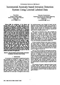
Figure 2. Plot of the trajectories from one of the 1000 data sets used for experiments in Section V-A. Blue trajectories are labelled as normal and red trajectories are labelled as anomalous. All anomalous trajectories in this data set were successfully detected by SNN-CAD with no false alarms. Table I AVERAGE ACCURACY FOR DIFFERENT OUTLIER MEASURES ON THE SIMULATED DATA (S ECTION V-A1). N OTE THAT ACCURACY RESULTS FOR SVM AND DISCORDS ARE 1 MINUS THE CORRESPONDING ERROR RATE REPORTED BY P ICIARELLI ET AL . [19]

Outlier measure − → SNN with S = δH SNN with S = δH SVM [19] Discords [20]

# of most similar neighbours considered k=1 k=2 k=3 k=4 k=5 96.59% 97.28%

97.12% 97.66%

97.05% 96.84% 97.63% 97.57% 96.30% [19] 97.04% [19]

96.72% 97.37%

authors calculated outlier scores for each of the 260 trajectories and checked if the 10 trajectories with highest outlier scores correspond to the 10 trajectories labelled as anomalous. The error rate, which is equivalent to 1 minus accuracy, was calculated for each method by averaging over the number of normal trajectories among the 10 trajectories with highest outlier scores. Since the nonconformity scores output by SNN correspond to the outlier scores output by the two other outlier measures, comparison is straightforward. Accuracy results for SNN and the corresponding accuracy results for SVM and discords reported by Piciarelli et al. are summarised in Table I. 2) On-line Learning and Sequential Anomaly Detection: − → In this section we evaluate SNN-CAD with S = δH for online learning and sequential anomaly detection in the simulated trajectories. The first objective is to demonstrate that anomalies can be detected with high sensitivity and low FAR before the complete trajectory has been observed, i.e. with a detection delay less than 16 data points. The second objective is to show that the FAR is well-calibrated and that the sensitivity to true anomalies increases during semi-supervised on-line learning. The setup is as follows: for each of 1000 sets of 260 simulated trajectories, we do the following. First we create an initial training set by randomly sampling 100 normal trajectories among the 250 labelled as normal. The remaining 160 trajectories (150 normal and 10 anomalous) are then randomly

158

30

Number of false negatives

25

20

15

10

5

0 100

150 200 Size of training set

250

Figure 3. Histogram showing frequency of false negatives (missed anomalies) based on size of training set for SNN-CAD during on-line learning and sequential anomaly detection in the simulated trajectory sets (Section V-A2).

permuted and sequentially presented to the algorithm. For each trajectory Ti = (z1 , ..., z16 ) , i = 1, ..., 160, we let SNN-CAD with k = 2 and  = 0.01 sequentially classify each incomplete trajectory Ti? = (z1 , ..., zm ) as normal or anomalous where m = 1, ..., 16. If Ti is a labelled anomaly and successfully detected as anomalous, it is simply discarded. In all other cases, the complete trajectory Ti = (z1 , ..., z16 ) is added to the training set before classifying the next trajectory Ti+1 , regardless of whether Ti is actually labelled as normal or anomalous. Thus, the algorithm operates in a semi-supervised mode where the true label for new examples are only given for those detected as anomalies; this corresponds to a setting where e.g. a human is alerted of trajectories detected as anomalous and either confirms or rejects each alarm. Results for the 1000 trajectory sets are as follows: the average sensitivity and FAR are 98% and 0.96%, respectively. The median detection delay is 6 out of 16 data points. Moreover, the number of false negatives based on the size of the accumulating training set is illustrated Figure 3.

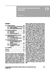
B. Experiment on Video Trajectories In this section we reproduce an experiment on a public data set of video trajectories3 . The data set consists of 239 labelled video motion trajectories where only two trajectories were visually identified as unusual behaviour [21]. The trajectories were extracted by Latecki et al. from IR surveillance videos using a motion detection and tracking algorithm [21]. Each trajectory is represented by five points in [x,y,time] space. A plot of all 239 trajectories is shown in Figure 4. Analogously to Pokrajac et al. [21], we calculate the outlier score for each of the 239 trajectories relative the rest using − → the SNN nonconformity measure with S = δH and k = 1. Sorting the resulting nonconformity scores, we observe that the two trajectories labelled as anomalous (see Figure 4) have the top two largest outlier scores. Hence, similar to Pokrajac [21] (and others) we achieve perfect accuracy on this data set. 3 www.cs.umn.edu/˜aleks/inclof

Figure 4. Plot of the 239 video surveillance trajectories extracted by Latecki et al. [21]. Blue correspond to normal trajectories. Two anomalous trajectories are indicated by the solid red and dashed red trajectories. Red solid correspond to a person walking left and then back right and dashed red correspond to person walking very slowly [21]. Both anomalies are detected by SNN-CAD with perfect accuracy, i.e. no false alarms (Section V-B).

C. Discussion It is clear from Table I that the SNN nonconformity measure based on Hausdorff distance is a relatively accurate outlier measure for the simulated trajectories. In particular, SNN with S = δH outperforms the other two trajectory outlier measures, regardless of the value of k. It is not surprising that δH − → performs better than δH for complete trajectories, since δH utilises all points from both trajectories during comparison; − → δH only considers distance to a subset of points from the other trajectory. However, δH is not appropriate for comparing incomplete trajectories and thus not applicable for sequential anomaly detection. Good performance was also observed on the video data set, where the SNN nonconformity measure − → with S = δH and k = 1 achieved perfect accuracy, similar to previously published algorithms (Section V-B). Considering the results from the on-line learning and sequential anomaly detection experiment (last paragraph of Section V-A2), we see that SNN-CAD often detects labelled anomalies before half the trajectory has been observed, at a high level of sensitivity (98%) and a low level of FAR (0.96%) which is well-calibrated. Moreover, Figure 3 indicates that the sensitivity increases as more training data is accumulated, even though 2% of the labelled anomalies are classified as normal and added to the training set. These outliers in the training set do not seem to affect FAR either. Intuitively, the approximation error of the implemented algorithm for calculating Hausdorff distance between two polygonal curves is bounded by the sampling distance of the points; the more sample points, the more accurate the calculation. It is possible that even better classification accuracy can be achieved by either considering a smaller sampling distance, or by calculating the exact Hausdorff distance using e.g. the algorithm proposed by Alt [16]. An advantage of the latter algorithm is that computational complexity can be reduced by compressing trajectories using e.g. the Douglas-Peucker algorithm for line simplification [22]. It should be stressed that relatively good accuracy results have been obtained on the public data sets without any param-

159

eter tuning. Compared to other algorithms, we argue that SNN− → CAD with S = δH has some principal properties that makes it more flexible and applicable in a wider range of applications: it does not require that trajectories are of equal length, it supports sequential anomaly detection in incomplete trajectories, it supports on-line learning, it has relatively few parameters, it has a well-calibrated false alarm rate and a principle way of setting the anomaly threshold that does not make any assumptions on the nature or frequency of anomalies. The property that trajectories need not be complete has in fact more general implications. We argue that the directed Hausdorff distance is not only robust to future data points that have not yet been observed; it also robust to previous data points that are missing due to delayed track initialisation, re-initialisation of previous track that was lost, etc. Limitations and Future Work: It would be interesting to evaluate how different amounts of anomalies in training data affect anomaly detection accuracy. For example, subtle anomalies may incorrectly be classified as normal and added to the training set during semi-supervised learning (see Section V-A2). Normal trajectories extracted from e.g. tracking systems may include noise due to incorrect measurements etc. Hence, further investigations regarding sensitivity to noise and anomalies, and methods for handling these should be pursued in future work. The Hausdorff distance is by definition insensitive to the ordering of the data points which may result in contra-intuitive matching. An example is two objects that follow the same path, hence small Hausdorff distance, yet they travel in opposite directions. This could be addressed by extending the feature space to also include current course. Another approach is to include relative time as an explicit feature; this would not only capture the direction but also the speed of the object. The CAD algorithm is quite general since it can be implemented using an arbitrary similarity/dissimilarity measure. Thus, considering anomaly detection from a general perspective, an interesting path for future work would be to investigate other nonconformity measure for CAD. VI. C ONCLUSION In this paper, we have introduced SNN-CAD which is a novel and parameter-light algorithm for on-line learning and automated anomaly detection. SNN-CAD is based on Conformal prediction and a key property that follows from this is that the false alarm rate is well-calibrated; if training data and new normal data are IID, the expected false alarm rate is equal to the specified anomaly threshold  ∈ (0, 1). No application specific anomaly threshold is required; the only design parameter in SNN-CAD is the dissimilarity measure. We have proposed two parameter-free trajectory dissimilarity measures based on the directed and undirected Hausdorff distance, respectively. An advantage of these measures is that they do not require that trajectories are of equal length. In particular, the measure based on directed Hausdorff distance is well-suited for sequential anomaly detection in incomplete trajectories. Experiments have been carried out using two public data sets with simulated trajectories and real video

trajectories, respectively. Results from reproduced experiments show that the proposed method achieves relatively good accuracy without any parameter tuning. Experiments also show that SNN-CAD can detect anomalies in incomplete trajectories while retaining a high level of sensitivity to true anomalies and a low false alarm rate. ACKNOWLEDGEMENTS This research has been supported by: the graduate school Intelligent Systems for Robotics, Automation and Process ¨ Control of the University of Orebro, Saab AB, and the University of Sk¨ovde, Sweden. The authors would like to acknowledge valuable feedback received from Klas Wallenius, Egils Sviestins and Thomas Kronhamn at Saab AB. R EFERENCES [1] V. Chandola, A. Banerjee, and V. Kumar, “Anomaly detection: A survey,” ACM Comput. Surv., vol. 41, no. 3, pp. 1–58, 2009. [2] D. Hawkins, Identification of Outliers. Chapman and Hall, 1980. [3] B. Morris and M. Trivedi, “A survey of vision-based trajectory learning and analysis for surveillance,” IEEE Trans. Circuits Syst. for Video Technol., vol. 18, pp. 1114–1127, August 2008. [4] A. Naftel and S. Khalid, “Classifying spatiotemporal object trajectories using unsupervised classifying spatiotemporal object trajectories using unsupervised learning in the coefficient feature space,” Multimedia Systems, vol. 12, no. 3, pp. 227–238, 2006. [5] X. Li, J. Han, K. Sangkyum, and H. Gonzalez, “Roam: Rule- and motifbased anomaly detection in massive moving object data sets,” in Proc. 7th SIAM Int. Conf. Data Mining, 2007. [6] C. Brax, L. Niklasson, and R. Laxhammar, “An ensemble approach for increased anomaly detection performance in video surveillance data,” in Proc 12th Int. Conf. Information Fusion, 2009. [7] R. Laxhammar, “Anomaly detection for sea surveillance,” in Proc 11th Int. Conf. Information Fusion, 2008. [8] F. Johansson and G. Falkman, “Detection of vessel anomalies - a bayesian network approach,” in Proc 3rd Int. Conf. Intelligent Sensors, Sensor Networks and Information Processing, 2007. [9] C. Piciarelli and G. Foresti, “On-line trajectory clustering for anomalous events detection,” Pattern Recognition Letters, vol. 27, 2006. [10] E. Keogh, S. Lonardi, C. Ratanamahatana, L. Wei, S.-H. Lee, and J. Handley, “Compression-based data mining of sequential data,” Data Mining and Knowledge Discovery, vol. 14, pp. 99–129, 2007. [11] M. Markou and S. Singh, “Novelty detection: a review - part 1: statistical approaches,” Signal Processing, vol. 83, no. 12, pp. 2481–2497, 2003. [12] S. Axelsson, “The base-rate fallacy and the difficulty of intrusion detection,” ACM Trans. on Inform. and Syst. Security, vol. 3, Aug 2000. [13] V. Vovk, A. Gammerman, and G. Shafer, Algorithmic Learning in a Random World. Springer-Verlag New York, Inc., 2005. [14] A. Gammerman and V. Vovk, “Hedging predictions in machine learning,” Computer Journal, vol. 50, no. 2, pp. 151–163, 2007. [15] G. Shafer and V. Vovk, “A tutorial on conformal prediction,” J. Mach. Learn. Res., vol. 9, pp. 371–421, 2008. [16] H. Alt, “The computational geometry of comparing shapes,” in Efficient Algorithms, Springer Berlin / Heidelberg, 2009. [17] R. Laxhammar and G. Falkman, “Conformal prediction for distributionindependent anomaly detection in streaming vessel data,” in Proc. 1st Int. Worksh. Novel Data Stream Pattern Mining Techniques, ACM, 2010. [18] T. Fawcett, “An introduction to roc analysis,” Pattern Recognition Letters, vol. 27, no. 8, pp. 861–874, 2006. [19] C. Piciarelli, C. Micheloni, and G. Foresti, “Trajectory-based anomalous event detection,” IEEE Trans. Circuits Syst. for Video Technol., vol. 18, pp. 1544 – 1554, November 2008. [20] E. Keogh, J. Lin, and A. Fu, “Hot sax: Efficiently finding the most unusual time series subsequence,” in Proc. 5th IEEE Int. Conf. Data Mining, 2005. [21] D. Pokrajac, A. Lazarevic, and L. Latecki, “Incremental local outlier detection for data streams,” in IEEE Symp. on Comp. Intell. and Data Mining (CIDM), 2007. [22] D. H. Douglas and T. K. Peucker, “Algorithms for the reduction of the number of points required to represent a digitized line or its caricature,” The Canadian Cartographer, vol. 10, no. 2, pp. 112–122, 1973.

160