WSEAS TRANSACTIONS onBIOLOGY and BIOMEDICINE
V. Glaser, A. Holobar, D. Zazula
Decomposition of Synthetic Surface Electromyograms Using Sequential Convolution Kernel Compensation V. Glaser, A. Holobar, D. Zazula Faculty of Electrical Engineering and Computer Science University in Maribor SLOVENIA
[email protected]
Abstract: - This paper reveals a sequential decomposition method based on Convolution Kernel Compensation (CKC). It operates in real time and can decompose linear mixtures of finite-length signals. Multiple-input multipleoutput (MIMO) signal model is used with finite channel responses and trains of delta pulses as inputs. Our approach compensates the channel responses and reconstructs the input pulse trains in real time, when samples of the observed signals become available. Two versions of the sequential decomposition were tested: sample-by-sample and multiple sample input. The time complexity of the two approaches, is analytically evaluated and supported by the experimental measurements. Performance tests on the synthetic surface electromyograms (sEMG) provide estimations of average rate and standard deviation of the reconstructed pulse trains for single motor units (MU). Key-Words: – Compound signal decomposition, Surface electromyogram, Real-time signal processing, ShermanMorrison-Woodbury matrix inversion, Sequential convolution kernel compensation (sEMG) channels. Due to low selectivity of surface electrodes, the measured signals are typically composed of contributions of many individual motor-units, whose action potentials (MUAPs) sum up to form highly interferential signal patterns [2]. A real EMG diagnostic value, whose application has been paved by the tradition of the needle EMG measurements, is based on the knowledge about its constituent components observed through individual MUAPs. Therefore, a strong need for reliable, robust and fast methods for decomposition of sEMG signals has recently emerged. One of the new promising decomposition approaches was developed in the System Software Laboratory at the University of Maribor and called Convolution Kernel Compensation (CKC) [1]. Its original derivation utilizes the correlation matrix built out of several simultaneous measurements that are processed in rather long segments. Hence, the underlying approach is batch, which does not meet the requirements for a fast, real-time decomposition. A sequential version of CKC (sCKC) was partially first derived in [3]. Although being computationally efficient, sCKC suffers from an inferior quality of decomposed signals. In this paper, we introduce a novel
1. Introduction Linear modelling of multiple observations excited by multiple input source signals has been shown to be of practical value in many different signal processing problems. Over the past decades, it has been applied to the fields of biomedicine, radar, sonar, image processing, speech separation, etc. In the field of electrophysiology, monitoring and diagnosing of the human neuromusclar system is frequently based on electromyograms (EMG). Different acquisition techniques have been proposed, enabling detection of electrical potentials in vicinity of muscle fibers or nerves. These measurable action potentials (AP) accompany muscle contractions and are controlled by the drive from the central nervous system (CNS). In normal conditions, a group of several tens or hundreds of muscle fibers is innervated by a single motoneuron, forming a basic functional unit of skeletal muscles, the so called motor unit (MU) [2]. In a muscle, several tens of MUs are active simultaneously, even at moderate contraction levels. Recently, multichannel acquisition systems became available, enabling noninvasive simultaneous recordings of up to several hundreds of surface EMG
ISSN: 1109-9518
143
Issue 7, Volume 5, July 2008
WSEAS TRANSACTIONS onBIOLOGY and BIOMEDICINE
V. Glaser, A. Holobar, D. Zazula
Adopting the model from Eq. (2) and the extensions from Eq. (3), an index of global pulse train activity can be defined as follows:
block-sequential CKC (bsCKC) method, which employs blocks of sEMG signals and combines the computation efficiency of sCKC with accuracy of batch CKC. The main goal of this paper is to analyse the sequential methods’ (sCKC and bsCKC) performance on synthetic sEMGs and their computational complexity. Our manuscript is organized as follows. In Section 2, a brief summary of the batch version of CKC is provided, followed by the derivations of sCKC and bsCKC in Section 3. Section 4 outlines the computational efficiency of both sCKC and bsCKC methods, whereas the performance of sCKC on synthetic sEMGs is discussed in Section V. The conclusions are presented in Section VI.
γ ( n ) = y T ( n ) ⋅ C #yy ⋅ y ( n ) ≈ s T ( n ) ⋅ C −s s1 ⋅ s ( n ) where # stands for pseudoinverse,
∑∑
h ij ( l ) s j ( n − l );
for transpose
matrix of noise-free source signals, si . Suppose we fix the premultiplying vector y (n0 ) in (4) to the position n0 , and rewrite the expression:
ν n 0 ( n ) = y T ( n 0 ) C #y y y ( n ) .
(5)
It was proven in [1] that when only the j-th source is active in time sample n0 , v n0 (n) yields the estimation of the pulse train from the j-th source:
vn0 ( n) ≈ s j (n) .
comprising superimpositions of responses from N sources: L −1
-1
of the noisy observations, y i , and C s s the correlation
The basic formulation of the CKC approach [1] uses a MIMO model of sEMG. It assumes M different observations xi = { xi (n); n = 0,1, 2,...} ; i = 1,..., M , each
N
and
and inverse, respectively, Cyy is the correlation matrix
2. Data Model and Convolution Kernel Compensation technique
xi (n ) =
T
(4)
(6)
Eq. (5) gives a recipe for decomposing a linear, convolutive mixture of pulse trains. Sensitivity of approximation (6) was explained in [1].
i = 1 ,..., M ,
j =1 l = 0
(1) where hij (l ) is a L-samples long response of the j-th
3. Sequential CKC with Single or Multiple Sample Input
source, as it appears in the i-th observation, whereas s j (n − l ) stands for a train of delta pulses from the j-th
Sequential CKC upgrades the batch CKC method by reducing the time support for computation of
source. When noisy observations are considered, (1) is modified as follows:
y i ( n ) = x i ( n ) + ω i ( n );
i = 1,..., M ,
correlation matrix Cyy from the entire signal segment to a single sample or block of consequent samples. It also
(2)
updates premultiplying vectors y T (n0 ) from Eq. (5) in iterative manner, as already explained in [3]. Both sequential methods comprise two major steps.
where ωi (n) stands for stationary, zero-mean white Gaussian random noise. In order to improve the ratio between the number of observations and the number of unknowns, the model (1) is extended with K-1 delayed repetitions of each observation:
In the first step, premultiplying vector y T (n0 ) is initialized and, afterwards, iteratively optimized to yield the filter fj of the single MU innervation pulse train sj [3]. This initialisation is explained in detail in Subsection 3.1. In the second step, the inverse of correlation matrix C#yy is calculated in iterative manner,
y( n) = ⎡⎣y1 ( n) , y1 ( n−1) ,...., y1 ( n−K +1) ,...., yM ( n) ,...., yM ( n−K +1)⎤⎦ . T
as outlined in Subsection 3.2.
(3)
ISSN: 1109-9518
144
Issue 7, Volume 5, July 2008
WSEAS TRANSACTIONS onBIOLOGY and BIOMEDICINE
V. Glaser, A. Holobar, D. Zazula
patterns are then mutually compared and all their repetitions discarded.
3.1 sCKC Initialisation Just like its batch version, sCKC uses activity index γ (n) to pinpoint the time instant n0 that defines the
3.2 Sequential Inverse of Correlation Matrix
starting filter:
Sequential CKC method relies on iterative calculation
f j = y (n0 ) ,
of the inverse C−yy1 , which proves to be computationally
(7)
highly intensive. To cope with this problem, the following Sherman-Morrison formula was proposed in [5] for the cases with the single-sample inputs:
where index j counts the number of different filters that produce different pulse trains. Instead of using entire y (n) , sCKC uses only the first S samples of
observations for the initialisation. In order to avoid the reidentification of the already identified pulse train, sCKC method prevents selection of another time instant nj within a region ε : L 2
L 2
ε = (n j − , n j + ) ,
( C y y + y ( n ) y ( n ) T ) − 1 = C −y y1 −
where y ( n ) is a vector of newly available samples of extended observations used for updating C−yy1 . When a block of P signal samples of extended observations Y P ( n ) = y ( n : n + P ) is available, (12) can be
where L is the maximal MUAP length (in samples). When all possible candidates for starting filters f j are
replaced by Sherman-Morrison-Woodbury formula [4]:
selected from activity index, sCKC gradually improves them using element-wise product between decompositions of initially recognised pulse trains
0 1
0
1
(Cyy + YP (n)YP (n)T )−1 = C−yy1 − C−yy1 YP (n)(I + YP (n)T C−yy1 YP (n))−1 YP (n)T C−yy1
(9)
estimated in [1] that already four proper positions ni combine in a pulse train which most probably belongs to a single source. Denoting this train with ν n0n1n2n3 (n) ,
decrease with iteration steps in (12) or (13).
suppose that pulses in this train appear at t0 ,K , t g −1 .
To avoid this problem, the inverse matrix must be renormalized by the number of available samples, which turns (10) into:
Then by averaging all the observation vectors in this time instants, an improved filter is constructed:
1 g −1 ∑ y (ti ) . g i =0
C −y 1y , n +1 =
(10)
−1 −1 ⎛ C yy C yy ⎞ T ⎜ ⎟ −1 y (n)y (n) C yy ⎜ ⎟ n n (n + 1)⎜ − −1 ⎟ n C ⎜ 1 + y (n)T yy y (n ) ⎟ n ⎝ ⎠
After initialization, sCKC checks for possible repetitions of the same pulse train using a threshold T j = max(ν ni ) ⋅ 0.85
(11)
and (11) into :
to discriminate the pulses in the j-th estimated train vni from the baseline noise. Resulting MU discharge
ISSN: 1109-9518
(13)
where I stands for matrix identity. Eq. (13) provides a theoretical framework for block-sequential CKC method. However, the application of (12) or (13) causes the estimated pulse amplitudes decrease in time, as shown in Fig. 1. This is mainly because (12) and (13) lack the normalization by the number of signal samples. As a result, the values of the matrix inverse C−yy1
which emphasizes only pulses triggered in a MUs active in time instants n0 and n1 , respectively. It was
fj =
1 + y ( n ) T C −y y1 y ( n )
(12)
(8)
ν n n (n) = ν n (n) ⋅ν n (n) ,
C −y y1 y ( n ) y ( n ) T C −y y1
145
Issue 7, Volume 5, July 2008
(14)
WSEAS TRANSACTIONS onBIOLOGY and BIOMEDICINE
V. Glaser, A. Holobar, D. Zazula
observation m0 onward, their pulses belong to the same
C−yy1,n+P =
pulse train:
⎛ C−yy1,n C−yy1,n C−yy1,n C−yy1,n ⎞ − YP (n)(I + YPT (n) YP (n))−1 YPT (n) ⎟ n n n ⎟⎠ ⎝ n (15)
( n + P) ⎜⎜
ν f (m) = ν f (m) ; m = m0 , m0 + 1K , j0
(17)
j1
whereas a different notation is used here for the pulse trains with subscripts identifying the premultiplying decomposition filter instead of a referential sample number.
where C −y1y ,n is the correlation matrix inverse of extended observations, calculated over n samples of observations.
Suppose that two pulse trainsν f j (m) and ν f j (m) 0
1
are equal for m = m0 K m0 + D , where D is a preselected threshold. In this case, the trains are considered produced by the same source, so that one of them can be discarded.
4. Computational Complexity To evaluate the decomposition speed, we estimated computational complexity analytically and also measured on a standard PC with 3000 MHz CPU and 2 GB of memory, as described in the sequel. In Subsection 4.1, analytical calculations for the sCKC time complexity is presented, while in Subsection 4.2 the results of its measurements follow.
Fig. 1: Estimated pulse train as obtained by sCKC without normalisation.
3.3 Sequential Filter Update Because the initialisation block of observations is rather short in comparison to the entire observation length, it is unlikely that the produced initialisation filters are sufficient for successful decompositions of pulses discharged in single MUs. Therefore, sequential filters have to be updated and improved after every new observation sample vector. Sequential filter update relies on running average:
f j , g +1 =
g ⋅ f j , g + y (t g +1 ) g +1
,
4.1 Analytical Estimate Complexity
of
Computational
The aim of sCKC is to be a real-time decomposition method. The most complex and most frequent operation is the update of the correlation matrix inverse, in particular when it is computed sample by sample. The complexity of optimized calculations of single-sample correlation matrix inverse using Sherman-Morrison formula is shown in Tables 1 and 2. Table 1 counts the number of multiplications, while Table 2 shows the number of additions. As already proven in [4], Sherman-Morrison formula has quadratic time complexity. In the Tables 3 and 4, the operations and their time complexity using Sherman-Morrison-Woodbury formula for block-sample updates of the correlation matrix inverse are depicted. Again, Table 3 counts the number of multiplications, while Table 4 shows the number of additions. As we can see, the time complexity of Sherman-Morrison-Woodbury formula is in general cubic.
(16)
where g is the number of observations deployed in the filter f j before the update with the new observation
y (t g +1 ) . 3.4 Sequential Removal of Multiple Pulse Train Recognitions Assume that f j0 and f j1 that produce trains ν f j (n) and 0
ν f (n) are improved in such way that from certain j1
ISSN: 1109-9518
146
Issue 7, Volume 5, July 2008
WSEAS TRANSACTIONS onBIOLOGY and BIOMEDICINE
V. Glaser, A. Holobar, D. Zazula
The times measured during our experimental runs of sCKC are gathered in the next section, and they comply with the analytical predictions.
Operation
Cy−y1,n =
A=Y C
Cy−y1,n =
C
( KM ) KM + 2 2 2 ( KM ) KM + 2 2
n
a⋅a B= T 1 + y (n + 1) ⋅ a T
C
(
= ( n + 1) C
−1 y y ,n
−B
Total:
Cy−y1,n = a=C
−1 y y ,n
C
D = BA1BT
2 P 2 KM 0
Total:
Cy−y1,n =
(
C −y1y ,n+1 = ( n + 1) Cy−y1,n − B Total:
n
2
D = BA1BT
( KM ) 2 KM + 2 2
Cy−y1,n − D
KM
Number of multiplications
( KM ) 2 KM + +1 2 2
1 C −YY ,n + P
( KM ) 2 + 2 KM + 1
Total:
0
2(KM ) P 2
P
−1
B = Cy−y1,n Y
Table 3: Number of multiplications in the application of Sherman-Morrison-Woodbury formula. P stands for the length of input blocks of observations, KM for the size of correlation matrix inverse, I is the identity, and A, A1, B, and D designate auxiliary matrices introduced for the sake of derivation.
ISSN: 1109-9518
C
A1 = ( I + A )
0
)
+ (KM ) + KM
−1 y y ,n
A = YT Cy−y1,n Y
n
a ⋅ aT B= 1 + y T (n + 1) ⋅ a
( KM ) 2 KM + 2 2 3 2 P + 3(( KM ) P ) + 2 P 2 KM +
Table 4: Number of additions in the application of Sherman-Morrison-Woodbury formula. P stands for the length input blocks of observations, KM for the size of correlation matrix inverse, I is the identity, and A, A1, B, and D designate auxiliary matrices introduced for the sake of derivation.
( KM ) 2 KM + 2 2 7 5 ( KM ) 2 + KM 2 2
Number of additions
⋅ y ( n + 1)
( P)3
(KM )2 P
1 C −YY ,n + P
Table 2: Number of additions in the application of Sherman-Morrison formula. KM stands for the size of correlation matrix inverse, n is the number of observations that contributed to the correlation matrix. Vector a and matrix B mean auxiliary variables used in the analytical derivation. −1 y y ,n
2
B = Cy−y1,n Y
Operation
Operation
2(KM ) P
Y
−1
( KM ) 2 + 2 KM
)
( KM ) 2 KM + 2 2
Cy−y1,n − D
2
a = Cy−y1,n ⋅ y ( n + 1)
−1 y y ,n +1
A1 = ( I + A )
Number of multiplications
−1 y y ,n
n −1 y y ,n
T
Table 1: Number of multiplications in the application of Sherman-Morrison formula. KM stands for the size of correlation matrix inverse, n is the number of observations that contributed to the correlation matrix. Vector a and matrix B mean auxiliary variables used in the analytical derivation. Operation
C
Number of multiplications
−1 y y ,n
(KM )2 P 2 P 2 KM
KM 2 0
3( KM ) 2 P + 2 P 2 KM + KM + P
4.2 Measured Time Complexity Three different experiments of computational complexity were performed on synthetic observations. In the first experiment, we measured the processing time needed to invert the correlation matrix when using different number of samples in the block inputs. In the second experiment, we investigated the impact of the size of correlation matrix on the processing time needed
147
Issue 7, Volume 5, July 2008
WSEAS TRANSACTIONS onBIOLOGY and BIOMEDICINE
V. Glaser, A. Holobar, D. Zazula
for its inversion. The third experiment focused on the overall processing times of bsCKC and sCKC methods, when decomposing random mixtures of synthetic pulse trains. Generated observations used in the experiments were produced from 10 different pulse trains, 10.000 samples long. The distance between pulses was normally distributed with a mean of 100 samples and variance of 30 samples. Channel responses were 8 samples long and the extension factor for CKC was set to 10 in all experiments. The first experiment was conducted on a set of 10 and 50 observations. The number of samples P in the input block Y P ( n ) ranged from 200 to 1000 in steps of
Fig. 3: Average computation time of matrix inverse for different input block lengths versus different matrix dimension. Standard deviations were negligibly small and are not reported. Simulations were conducted on a standard PC with 3000 MHz CPU and 2 GB of memory.
100 samples. Forty Monte-Carlo runs were conducted with different input pulse trains and channel responses generated randomly for each simulated value of P, whereas the size of correlation matrix was set to 100×100 and 500×500, respectively. Results, averaged over all simulation runs, are depicted in Fig. 2. In all the cases, standard deviations were negligibly small and are not reported.
In the second experiment, length of input blocks Y P ( n ) was set equal to 1, 100, 300, 400 and 500 samples, respectively. Different sizes of correlation matrix were simulated, ranging from 100×100 to 1000×1000. Twenty Monte-Carlo runs were conducted with different observations, as described for the first experiment, per each matrix size and each length of input block Y P ( n ) . The results are shown in Fig. 3. Now take the analytical expression for the number of multiplications in Sherman-Morrison-Woodbury formula from Table 3. When KM is significantly smaller than P, time complexity of Sherman-MorrisonWoodbury formula is cubic, but when KM surpasses P significantly, the formula becomes quadratic, which can be best seen in Fig. 3 for P=500 samples. In the last experiment, 10, 30 and 50 simulated observations were used. The initial window was 500 samples long. Twenty Monte-Carlo runs were conducted for three matrix dimensions versus different input block lengths. The results are depicted in Fig. 4.
Fig. 2: Average computation time of matrix inverse with block inputs of size from 200 to 1000 samples. Standard deviations were negligibly small and are not reported. Simulations were conducted on a standard PC with 3000 MHz CPU and 2 GB of memory.
ISSN: 1109-9518
148
Issue 7, Volume 5, July 2008
WSEAS TRANSACTIONS onBIOLOGY and BIOMEDICINE
V. Glaser, A. Holobar, D. Zazula
where ν f (n) is the decomposition of pulse train s j0 . j0
All such pulses are termed missed pulses (false s j0 (n0 ) = 0 and negative). Secondly, when ν f j (n0 ) > T j0 , 0
positive).
And
we
have
thirdly,
misplaced when
pulses
s j0 (n0 ) = 1
(false and
ν f j (n0 ) > T j0 this means a correct pulse recognition 0
(true positive). We verified our decomposition method on synthetic sEMGs and studied the influence of noise corruption on the decomposition performance. Recognition rates and rates of missed and misplaced pulses are presented in subsequent sections.
Fig. 4: Average decomposition time when using the bsCKC method versus the input block size. Standard deviations were negligibly small and are not reported.
5.1 Synthetic sEMG A sEMG model [6] from the LISiN Laboratory in Torino was used to generate synthetic signals. Constant contraction forces, planar volume conductor muscle model [7], and double differential uptake electrodes were simulated. Innervation firing patterns were sampled by 4096 Hz, while the sEMG signal sample frequency was 1024 Hz. Firing patterns were 122880 samples long, producing sEMGs with 30720 samples. Three different sets of sEMGs were generated, with 5, 10 and 20 simulated active MUs. Each set comprise 5 different sEMGs.
Assume also we have observations with Q samples and S samples are used for the initialization and P samples for every input block. Then the number of required updates of correlation matrix inverse can be calculated as
R=
(Q − S ) . P
(19)
The number of required updates R decreases with P, whereas the time needed for calculation of each update of correlation matrix inverse increases with P, as shown in previous experiments. For small values of P, the number of required updates R has a dominant effect on the total CKC processing time. Eventually, negative effect of increased block size P overrides the positive effect of smaller number of inverse updates R, causing the entire bsCKC processing time to increase with P. The optimal performance of bsCKC is achieved when
KM KM