presented into a nonlinear semidefinite programming problem. A sequential ... programming method is proposed which has the global convergent property.
Sequential Semidefinite Program for Maximum Robustness Design of Structures under Load Uncertainties 1
Y. Kanno 2 and I. Takewaki 3
Communicated by K.K. Choi
1
The authors are grateful to the Associate Editor and two anonymous referees for handling the paper efficiently as well
as for helpful comments and suggestions.
2
Assistant Professor, Department of Urban and Environmental Engineering, Kyoto University, Kyoto, Japan.
3
Professor, Department of Urban and Environmental Engineering, Kyoto University, Kyoto, Japan.
Abstract.
A robust structural optimization scheme as well as an optimization algorithm are presented based on the robustness function. Under the uncertainties of external forces based on the info-gap model, the maximization problem of the robustness function is formulated as an optimization problem with infinitely many constraints. By using the quadratic embedding technique of uncertainty and the S-procedure, we reformulate the problem presented into a nonlinear semidefinite programming problem. A sequential semidefinite programming method is proposed which has the global convergent property. It is shown through numerical examples that optimum designs of various linear elastic structures can be found without any difficulty.
Key Words.
Robust optimization, info-gap model, semidefinite program, structural optimization, successive linearization method
1. Introduction In mechanical engineering, the robust optimal design of various structures has received increasing attention. Based on the stochastic uncertainty model of mechanical parameters, various methods were proposed for reliability-based optimization. The structural optimization by minimizing the failure probability was studied (Ref. 1). In order to reduce the computational cost in evaluation of the failure 1
probability, the reliability index approach was utilized (Ref. 2). Various formulations for sensitivity analysis of probabilistic constraints were also proposed (Ref. 3, 4). Doltsinis and Kang (Ref. 5) performed a multi-objective optimization so as to minimize both the expected value and the standard deviation of the goal performance. On the other hand, as a non-probabilistic but bounded uncertainty model, the so-called convex model approach has been well established (Ref. 6), with which Pantelides and Ganzerli (Ref. 7) proposed a method for robust truss optimization. A unified methodology of robust counterpart of a broader class of convex optimization problems was developed by Ben-Tal and Nemirovski (Ref. 8), which was applied to robust compliance minimization of trusses (Ref. 9). Koˇcvara et al. (Ref. 10) performed a free-material design under multiple loadings by using a cascading technique. Han and Kwak (Ref. 11) attempted to find the design which minimizes a magnitude of sensitivity coefficients of the performance functions. Based on the semidefinite programming relaxation, Calafiore and El Ghaoui (Ref. 12) proposed a method for finding the ellipsoidal bound of the solution set of uncertain linear equations. Based on the info-gap decision theory, the concept of robustness function was proposed by BenHaim (Ref. 13). The robustness function expresses the greatest level of non-probabilistic uncertainty at which any constraint in a mechanical system cannot be violated. The robustness function has the advantage, compared with reliability analyses based on stochastic uncertainty models, such that engineers do not have to estimate neither the level of uncertainty nor the probabilistic distribution of 2
uncertain parameters, i.e., the robustness function does not require any information on statistical variation of the uncertain parameters of a mechanical system, which is often difficult to obtain practically. The authors proposed an efficient technique for computing a lower bound of robustness function for a given truss design (Ref. 14). However, to the authors’ knowledge, neither an algorithm nor a methodology has been presented for robust structural optimization based on the robustness functions. Let g : Rn �→ Rk , h : R×Rn ×Rz �→ Rm , and Z : R �→ P(Rz ), where P(Rz ) denotes the set consisting of all subsets of Rz . Assume that Z(α) is bounded and convex for any α and that Z(α1 ) ⊂ Z(α2 ) holds if α1 < α2 . Our goal is to solve an optimization problem having the form of
max {α : h(α, a, ζ) ≥ 0, ∀ζ ∈ Z(α), g(a) ≥ 0} , α,a
(1)
which corresponds to the problem finding a structural design which maximizes the robustness function over some constraints on mechanical performance; see Section 4. Here, a ∈ Rn and ζ ∈ Rz denote the design variables and the unknown-but-bounded parameters, respectively. We shall make further assumptions on h and Z; see Sections 2.1 and 2.2. The robustness function � α(a) at a given design a is defined by
� α(a) = max {α : h(α, a, ζ) ≥ 0, ∀ζ ∈ Z(α)} ; α
(2)
see Section 2.3 for a rigorous definition of the robustness function. It should be emphasized that Problems (1) and (2) have the infinitely many constraints, because h(α, a, ζ) ≥ 0 should hold for infinitely many ζ satisfying ζ ∈ Z(α). To overcome this difficulty, 3
we first show in Section 3 that Problem (2) can be equivalently reformulated into the semidefinite programming (SDP) problem (Ref. 15). Secondly, in Section 4, Problem (1) is reformulated into a socalled nonlinear SDP problem (Ref. 16), which is the maximization problem of a linear function over the constraints such that the matrix defined as the nonlinear function of variables should be positive semidefinite. Based on the successive linearization method (Ref. 17, 18), we propose an algorithm solving Problem (1) with the global convergence property under certain assumptions, at each iteration of which we solve the (linear) SDP problems by using the primal-dual interior-point method (Ref. 15). This paper is organized as follows. In Section 2, in order to make this paper self-contained, we formulate the robustness function in the form of Problem (2). We also briefly introduce SDP (Ref. 15) and some technical results on the linear matrix inequality. Section 3 shows that the robustness function of a structure with a fixed design is obtained by solving an SDP problem. In Section 4, we define the maximization problem of robustness function as a novel concept of robust structural design, and reformulate it as a nonlinear SDP problem. An algorithm based on the successive linearization method is also proposed. Section 5 investigates the global convergent behavior of our algorithm. Numerical experiments are presented in Section 6 for truss structures, while conclusions are drawn in Section 7.
2. Preliminaries In this paper, all vectors are assumed to be column vectors. For vectors p ∈ Rn and q ∈ Rm , we often simplify (p� , q�)� as (p, q). The standard Euclidean norm �p�2 = (p� p)1/2 of a vector p ∈ Rn
4
is often abbreviated by �p�. For P ∈ Rn×n , tr(P) denotes the trace of P, i.e., the sum of the diagonal elements of P. We write Diag(p) for the diagonal matrix with the vector p ∈ Rn on its diagonal. This notation is extended to general block diagonal matrices: if P1 , P2 , . . . , Pk are symmetric matrices, then Diag(P1 , . . . , Pk ) denotes the block diagonal matrix with the P1 , P2 , . . . , Pk down its diagonal. The set of all n × n real symmetric matrices is denoted by Sn . Let Sn+ ⊂ Sn denote the set of all positive semidefinite matrices. We write P O and P Q, respectively, if P ∈ Sn+ and P − Q ∈ Sn+ . For a set X, P(X) denotes its power set, i.e., a set consisting of all subsets of X. Let Rn+ ⊂ Rn and Ln+ ⊂ Rn denote the non-negative orthant and the second-order cone (Ref. 21), respectively, defined as � � � Rn+ = {p = (pi ) ∈ Rn | pi ≥ 0, i = 1, . . . , n} and Ln+ = (p�0 , p�1 )� �� p0 ≥ �p1 �2 , p0 ∈ R, p1 ∈ Rn−1 . Let P : Rm �→ Sn and Q ∈ Sn . The derivative DP(x ) of the mapping P(·) at x ∈ Rm is defined such that DP(x )z is a linear function of z = (zi ) ∈ Rm given by
DP(x )z =
m � i=1
� ∂P(x) �� � zi . ∂xi �x=x
Then we obtain � � m �� ∂(Q • P(x)) �� �� R � Q • DP(x ) = . ∂xi x=x i=1 m
�
2.1. Mechanical Performance Constraints d
Consider a finite-dimensional linear elastic structure subjected to the nodal loads f ∈ Rn , where nd is the total number of degrees of freedom. Small displacements and small strains are assumed. m
Let a = (ai ) ∈ Rn denote the vector of design variables, e.g., the cross-sectional areas of a truss, the 5
d
thickness of a plate discretized into finite elements, etc. The stiffness matrix is denoted by K(a) ∈ Sn . d
The displacement vector u ∈ Rn is found from the system of equilibrium equations
K(a)u = f,
(3)
where f is assumed to be independent of a. In this paper, we consider mechanical performance of structures that can be expressed by some polynomial inequalities in terms of displacements u, namely, structures should satisfy
q(u) ≥ 0,
(4)
where q(·) is a vector-valued polynomial function. We may suppose that q depends on the paramr
eters rc ∈ Rn representing the critical levels of performance, where nr denotes the number of these parameters. It is known that any single polynomial inequality can be converted into a system of (a finite number of) quadratic inequalities; see, e.g., Kojima and Tunc¸el (Ref. 19). Hence, (4) can be rewritten into some quadratic inequalities in terms of u. Let Hl : Rn �→ Sn +1 . Define a point-to-set mapping r
r
d
d
F : Rn �→ P(Rn ) by
⎫ ⎧ �� ⎛ ⎞� ⎛ ⎞ ⎪ ⎪ ⎪ ⎪ � ⎜ ⎜ ⎟ ⎟ ⎪ ⎪ ⎜⎜⎜ ⎟⎟⎟ ⎜⎜⎜ ⎟⎟⎟ ⎪ ⎪ � ⎪ ⎪ � ⎪ ⎪ ⎜ ⎜ ⎟ ⎟ ⎪ ⎪ ⎜ ⎜ ⎟ ⎟ � ⎪ ⎪ u u ⎜ ⎜ ⎟ ⎟ ⎪ ⎪ � ⎜ ⎜ ⎟ ⎟ ⎪ ⎪ d ⎜ ⎜ ⎟ ⎟ ⎨ � ⎟ ⎟ c n ⎜ c ⎜ c⎬ ⎜ ⎜ ⎟ ⎟ � H (r ) F (r ) = ⎪ . u ∈ R ≥ 0, l = 1, . . . , n ⎜ ⎜ ⎟ ⎟ ⎪ l ⎜ ⎜ ⎟ ⎟ ⎪ ⎪ � ⎜ ⎜ ⎟ ⎟ ⎪ ⎪ ⎜⎜⎜ ⎟⎟⎟ ⎜⎜⎜ ⎟⎟⎟ � ⎪ ⎪ ⎪ ⎪ � ⎪ ⎪ ⎜⎜⎝ ⎟⎟⎠ ⎪ ⎪ �� ⎜⎜⎝1⎟⎟⎠ ⎪ ⎪ ⎪ ⎪ 1 ⎪ ⎪ ⎭ ⎩ �
(5)
Then (4) can be equivalently rewritten in the form of
u ∈ F (rc ). 6
(6)
Example 2.1. As a simple example, we demonstrate to reformulate the stress constraints of trusses into (6). For a truss, it is known that the stress σi of the ith member is written as σi (u) = di� u, where d
di ∈ Rn is a constant vector. The conventional stress constraints are given as
σi ≤ σi ≤ σi ,
i = 1, . . . , nm ,
(7)
where R � σi < 0 and R � σi > 0 denote the lower and upper bounds of stress of the ith member, respectively. The constraints (7) can be embedded into the form of (6) with ⎫ ⎧ �� ⎛ ⎞� ⎛ ⎞⎛ ⎞ ⎪ ⎪ ⎪ ⎪ � ⎜ ⎟ ⎜ ⎜ ⎟ ⎟ ⎪ ⎪ ⎟⎟⎟ ⎜⎜⎜ ⎟⎟⎟ ⎪ ⎪ �� ⎜⎜⎜ ⎟⎟⎟ ⎜⎜⎜ σ + σ ⎪ ⎪ i ⎪ ⎪ i � ⎜ ⎟ ⎜ ⎜ ⎟ ⎟ ⎪ ⎪ ⎟⎟⎟ ⎜⎜⎜u⎟⎟⎟ �� ⎜⎜⎜u⎟⎟⎟ ⎜⎜⎜ −di di ⎪ ⎪ d i ⎪ ⎪ ⎪ ⎪ ⎟⎟ ⎜⎜⎜ ⎟⎟⎟ ⎜⎜ ⎟⎟⎟ ⎜⎜⎜ ⎨ 2 ⎟ nd � ⎜ m⎬ � F (σ, σ) = ⎪ , u ∈ R ≥ 0, i = 1, . . . , n ⎜ ⎟ ⎜ ⎜ ⎟ ⎟ ⎪ ⎜ ⎟ ⎜ ⎜ ⎟ ⎟ ⎪ ⎪ �� ⎜⎜ ⎟⎟ ⎜⎜ ⎟⎟⎟ ⎜⎜⎜ ⎟⎟⎟ ⎪ ⎪ ⎪ ⎪ ⎜⎜⎜ ⎟⎟⎟ ⎜⎜⎜ σi + σ ⎪ ⎪ ⎟ ⎜ ⎟ � ⎪ ⎪ ⎟⎜ ⎟ ⎪ ⎪ i � �� ⎜⎝1⎟⎠ ⎜⎝ ⎪ ⎪ ⎪ ⎪ di −σi σi ⎟⎠ ⎜⎝1⎟⎠ ⎪ ⎪ ⎭ ⎩ � 2 where nc = nm . Note that (σ, σ) is regarded as the levels of performance in (7). Hence, we have rc = (σ, σ) with nr = 2nm .
�
For general structures discretized into finite elements, it is easy to see that conventional upper bound constrains of displacements can be represented in the form of (6). Moreover, for two- or threedimensional structures discretized into isoparametric finite elements, our framework can deal with the stress constraints based on the Huver–von Mises yield condition (Ref. 20, Section 2.3). Let σ ∈ Sdim denote the symmetric stress tensor, where dim ∈ {2, 3}. At the jth sampling point of quadrature, the stress constraint is written as
1 2 tr(σ j σ j ) − (tr(σ) j )2 ≤ rcj σ2Y j , 3 3
7
(8)
where σY j is the flow stress and 0 < rcj ≤ 1 is regarded as a safety factor. Since σ j is a linear function of u, (8) can be embedded into (6).
2.2. Uncertainty Model Throughout the paper, we assume that f in (3) has uncertainty and that K(a) is known precisely. d Let � f ∈ Rn denote the nominal value of f . The uncertainty of f is expressed by using an unknown-
d
but-bounded vector ζ ∈ Rn . Suppose that f depends on ζ affinely, i.e., f = � f + ζ.
(9)
Let Γ ∈ Rn ×n be a constant matrix. Define Z : R+ �→ P(Rn ) by d
d
d
� � Z(α) = ζ ∈ R � α ≥ �Γζ�2 . �
nd ��
(10)
For a given α, the uncertain vector ζ is assumed to be running through the uncertainty set Z(α) defined by (10). As an example, we may simply choose the identity matrix as Γ; then ζ ∈ Z(α) runs around the origin with the radius of α. Thus, α is regarded as a level of uncertainty. For a fixed α > 0, the ellipsoidal uncertainty model of f defined by (9) and (10) is essentially same as that introduced by Ben-Tal and Nemirovski (Ref. 9) for robust compliance minimization of trusses. However, α is treated as a variable parameter in our context; see Section 2.3 for more details. We make the following assumptions throughout the paper:
Assumption 2.1. rank(Γ) = nd . Assumption 2.2. For each l = 1, . . . , nc , Hl in (5) is not positive semidefinite. 8
Assumption 2.1 guarantees that Z is bounded for any finite α ≥ 0. Assumption 2.2 does not lose generality, because Hl O implies that the inequality (4) becomes redundant. We shall use further two assumptions in Section 5:
Assumption 2.3. � f � 0.
Assumption 2.4. The stiffness matrix K(a) is a linear function of design variables a.
Assumption 2.3, together with Assumption 2.1, guarantees Γ � f � 0. Assumption 2.4 holds for, e.g., structures such as trusses, plates with in-plane deformation, frames and plates with sandwich cross-sections, etc. Note that Assumption 2.3 and Assumption 2.4 will be required only in Section 5 for the convergence analysis of an algorithm presented in Section 4. It is easy to see that the uncertainty set Z(α) defined by (10) obeys a so-called info-gap model (Ref. 13) under Assumption 2.1. Especially, it satisfies the axioms of nesting and contraction (Ref. 13, Section 2.5), i.e., we see (i) Z(α1 ) ⊂ Z(α2 ) if 0 ≤ α1 < α2 ; (ii) Z(0) = {ζ| ζ = 0}. From (9) and (10) it follows that the system (3) of uncertain equilibrium equations is reduced to
K(a)u = � f + ζ,
ζ ∈ Z(α).
(11)
d
Let U(α, a) ⊆ Rn denote the set of all the possible solutions to (11), i.e., U is the point-to-set mapping m
d
U : R+ × Rn �→ P(Rn ) defined by � � � d� U(α, a) = u ∈ Rn �� (11) .
9
(12)
2.3. Robustness Function The robustness function represents the maximum value of α at which the constraints (6) on mechanical performance cannot be violated (Ref. 13, Chapter 3). Consider the following semi-infinite programming problem in the variable α:
α∗ = max {α : U(α, a) ⊆ F (rc )} , α∈R+
(13)
where F and U have been defined in (5) and (12), respectively. Here, by semi-infinite we mean optimization problems having a finite number of scalar variables and possibly an infinite number of inequality constraints. The constraint of Problem (13) implies that u ∈ F (rc ) should be satisfied by any u solving (11) for some ζ ∈ Z(α). By taking infinitely many ζ satisfying ζ ∈ Z(α), the constraint of Problem (13) can be rewritten as infinitely many quadratic inequalities. m
c
The robustness function � α : Rn × Rn �→ (−∞, +∞] associated with the constraints (6) is defined as ⎧ ⎪ ⎪ ⎪ ⎪ ⎪ ⎪ ⎪ ⎪ ⎪ α∗ , if Problem (13) is feasible, ⎪ ⎪ ⎪ ⎨ � α(a, rc ) = ⎪ ⎪ ⎪ ⎪ ⎪ ⎪ ⎪ ⎪ ⎪ ⎪ ⎪ ⎪ ⎩0, if Problem (13) is infeasible. In what follows, � α(a, rc ) is often abbreviated by � α. For the two different vectors of cross-sectional m
m
areas a1 ∈ Rn and a2 ∈ Rn , we say that a1 is more robust than a2 if � α(a1 , rc ) > � α(a2 , rc ). Let � � � �� α, a1 ) at ζ 1 ∈ Z(� α). If there exists an l ∈ {1, . . . , nc } satisfying (u1 )� , 1 Hl (rc ) (u1 )� , 1 = 0, u1 ∈ U(� then we say that ζ 1 is the worst case. Note that there exists typically more than a single worst case. 10
Thus, the robustness function � α can be obtained by solving the optimization problem (13). Unfortunately, Problem (13) is numerically intractable, because it has infinitely many constraints. This motivates us to investigate in Section 3 an SDP reformulation of Problem (13).
2.4. Semidefinite Program Let Ai ∈ Sn , i = 1, . . . , m, C ∈ Sn , and b = (bi ) ∈ Rm be constant matrices and a constant vector. The semidefinite programming (SDP) problem refers to the optimization problem having the form of
min {tr(CX) : tr(Ai X) = bi , i = 1, . . . , m, Sn � X O} , X
(14)
where X is a variable matrix (Ref. 15). The dual of Problem (14) is formulated in the variables y ∈ Rm as ⎧ ⎫ m ⎪ ⎪ � ⎪ ⎪ ⎨ � ⎬ y : C − A y O max ⎪ b , ⎪ i i ⎪ ⎪ ⎭ y ⎩
(15)
i=1
which is also an SDP problem. SDP has attracted considerable attention for its wide fields of application (Ref. 21–23). The primal-dual interior-point methods, which were developed for the linear program at first, have been naturally extended to SDP (Ref. 15). It is theoretically guaranteed that the primal-dual interior-point method converges to the optimal solutions of the pair of SDP problems (14) and (15) within the number of arithmetic operations bounded by a polynomial of m and n (Ref. 15, 21).
2.5. Technical Lemmas The reminder of this section is devoted to introducing some technical results that will be used in 11
the following sections.
Lemma 2.1. (Homogenization). Let Q ∈ Sn , p ∈ Rn , and r ∈ R. Then the following two conditions are equivalent:
(a)
(b)
⎞⎛ ⎞ ⎛ ⎞� ⎛ ⎟⎟⎟ ⎜⎜⎜ ⎟⎟⎟ ⎜⎜⎜ ⎟⎟⎟ ⎜⎜⎜ ⎟⎜ ⎟ ⎜⎜⎜ ⎟⎟⎟ ⎜⎜⎜ ⎜⎜⎜ x⎟⎟⎟ ⎜⎜⎜ Q p⎟⎟⎟⎟⎟ ⎜⎜⎜⎜⎜ x⎟⎟⎟⎟⎟ ⎟⎟⎟ ⎜⎜⎜ ⎟⎟⎟ ≥ 0, ⎜⎜⎜⎜ ⎟⎟⎟⎟ ⎜⎜⎜⎜ ⎟⎟ ⎜⎜ ⎟⎟ ⎜⎜⎜ ⎟⎟⎟ ⎜⎜⎜ ⎜⎜⎜ ⎟⎟⎟ ⎜⎜⎜ � ⎟⎟⎟⎟⎟ ⎜⎜⎜⎜⎜ ⎟⎟⎟⎟⎟ ⎝1⎠ ⎝ p r ⎠ ⎝1⎠
∀x ∈ Rn ;
⎞ ⎛ ⎟⎟⎟ ⎜⎜⎜ ⎟ ⎜⎜⎜ ⎜⎜⎜ Q p⎟⎟⎟⎟⎟ ⎟⎟⎟ O. ⎜⎜⎜⎜ ⎟⎟ ⎜⎜⎜ ⎜⎜⎜ � ⎟⎟⎟⎟⎟ ⎝p r ⎠
Proof. See Lemma A.3 in Calafiore and El Ghaoui (Ref. 12).
�
Lemma 2.2. (S-Procedure). For Qi ∈ Sn , pi ∈ Rn , and ri ∈ R, i = 0, 1, define fi : Rn �→ R as fi (ξ) = ξ � Qi ξ + 2p�i ξ + ri . The implication
f1 (ξ) ≥ 0
=⇒
f0 (ξ) ≥ 0
holds if and only if there exists a nonnegative parameter τ such that
f0 (ξ) − τ f1 (ξ) ≥ 0,
∀ξ ∈ Rn .
Proof. See Theorem 4.3.3 in Ben-Tal and Nemirovski (Ref. 21).
Lemma 2.3. (Schur Complement). Let P ∈ Sn be positive definite, and let Q ∈ Sm . Define X by ⎞ ⎛ ⎟⎟ ⎜⎜⎜ ⎜⎜⎜⎜P A� ⎟⎟⎟⎟⎟ ⎟⎟⎟ ⎜⎜ ⎟⎟⎟ . X = ⎜⎜⎜⎜⎜ ⎟⎟⎟ ⎜⎜⎜ ⎟⎟ ⎜⎜⎝ A Q ⎟⎠ Then X O if and only if Q − AP−1 A� O. 12
�
�
Proof. See Lemma 4.2.1 in Ben-Tal and Nemirovski (Ref. 21).
3. SDP Formulation of Robustness Function Throughout this section, we assume U(0, a) ⊆ F for a given a, i.e., Problem (13) has the nonempty feasible set. Define Ω : R × Rn �→ Sn +1 by m
d
⎞ ⎛ ⎟⎟⎟ ⎜⎜⎜ ⎜⎜⎜ � � �⎟ ⎜⎜⎜−K(a)Γ ΓK(a) K(a)Γ Γ f ⎟⎟⎟⎟⎟ ⎟⎟⎟ . Ω(t, a) = ⎜⎜⎜⎜⎜ ⎟⎟⎟ ⎜⎜⎜ ⎟⎟⎟ ⎜⎜⎝ �� � t− � f � Γ� Γ � f ⎟⎠ f Γ ΓK(a)
(16)
The following result shows that the robustness function � α can be obtained by solving an SDP problem:
m
c
α(a, rc ) is obtained by Proposition 3.1. For given a ∈ Rn and rc ∈ Rn , the robustness function � c
solving the following SDP problem formulated in the variables (t, ρ) ∈ R × Rn :
� α(a, rc )2 = max {t : ρl Hl (rc ) Ω(t, a), l = 1, . . . , nc , ρ ≥ 0} . t,ρ
(17)
Proof. Since ζ ∈ Z(α) is satisfied if and only if ζ � Γ� Γζ ≤ α2 , we see that u ∈ U(α, a) is equivalent to �
� � �� f ≤ α2 . K(a)u − � f Γ� Γ K(a)u − �
Consequently, by using the definition (16) of Ω and K(a) = K(a)� , we obtain ⎧ ⎫ �� ⎛ ⎞� ⎛ ⎞ ⎪ ⎪ ⎪ ⎪ � ⎜ ⎜ ⎟ ⎟ ⎪ ⎪ ⎜ ⎜ ⎟ ⎟ ⎪ ⎪ �� ⎜⎜ ⎟⎟ ⎜ ⎟ ⎪ ⎪ ⎜ ⎟ ⎪ ⎪ ⎜⎜u⎟⎟⎟ ⎜⎜u⎟⎟⎟ ⎪ ⎪ ⎜ ⎜ � ⎪ ⎪ ⎪ ⎪ � ⎜ ⎜ ⎟ ⎟ ⎪ ⎪ d ⎜ ⎜ ⎟ ⎟ ⎨ ⎜ ⎟ ⎟ n �⎜ 2 ⎜⎜ ⎟⎟⎟ Ω(α , a) ⎜⎜⎜ ⎟⎟⎟ ≥ 0 ⎬ � U(α, a) = ⎪ u ∈ R . ⎜ ⎪ ⎪ ⎪ � ⎜⎜⎜ ⎟⎟⎟ ⎜⎜⎜ ⎟⎟⎟ ⎪ ⎪ � ⎪ ⎪ ⎪ ⎪ �� ⎜⎜⎜ ⎟⎟⎟ ⎪ ⎪ ⎜⎜⎜⎝ ⎟⎟⎟⎠ ⎪ ⎪ ⎪ ⎪ ⎪ ⎪ 1 �� ⎝1⎠ ⎪ ⎪ ⎩ ⎭
13
(18)
The constraint of Problem (13) is equivalently rewritten as
u ∈ U(α, a)
=⇒
u ∈ F (rc ).
(19)
It follows from (18), the S-lemma (Lemma 2.2) and the homogenization (Lemma 2.1) that (19) holds if and only if
∃τl ≥ 0
s.t.
Hl (rc ) τl Ω(α2 , a),
l = 1, . . . , nc .
(20)
Recall that Hl (rc ) � O has been assumed in Assumption 2.2, which implies that τl = 0 does not satisfy (20). Hence, by putting ρl = 1/τl , l = 1, . . . , nc , the condition (20) is reduced to
∃ρl ≥ 0
s.t.
ρl Hl (rc ) Ω(α2 , a),
l = 1, . . . , nc .
Consequently, Problem (13) is equivalently rewritten as � � � α(a, rc ) = max α : ρl Hl (rc ) Ω(α2 , a), l = 1, . . . , nc , ρ ≥ 0 . α,ρ
(21)
We can see in Problem (21) that maximizing α is equivalent to maximizing α2 , which concludes the �
proof.
The reduction of (19) to (20) is motivated by an extension of the idea found in the proof of Theorem 1 in (Ref. 12). It is of interest to note that Problem (17) can be embedded into a dual standard form of SDP problem (15) with m = nc + 1 and n = nc + nc (nd + 1). Thus, m and n are bounded by polynomials of nd and nc . The primal-dual interior-point method can find a global optimal solution of SDP with the 14
number of arithmetic operations bounded by a polynomial of m and n (Ref. 15). Hence, Problem (17) can be solved with polynomial time complexity of nd and nc in spite of the fact that the original problem (13) has infinitely many constraints.
4. Maximization Problem of Robustness Function We observed in Section 2.3 that the structure having a larger robustness function is regarded as to be more robust. In this section, we attempt to find the design variables vector a which maximizes the robustness function � α(a, rc ). We call this structural optimization problem the maximization problem of robustness function. Consider the conventional constraints on a such as the upper and lower-bound constraints of a m
g
and upper-bound constraint of structural volume. Letting g : Rn �→ Rn be a smooth function, these constraints may be written in the form of
g(a) ≥ 0.
(22)
Note that g(a) involves neither u nor f . For the given rc and g, the maximization problem of robustness function is formulated as � � max � α(a, rc ) : g(a) ≥ 0 . a
(23)
m
In what follows, the argument rc is often omitted for brevity. Assume that there exists a ∈ Rn
satisfying � α(a, rc ) > 0. Then the objective function of Problem (23) can be replaced by � α(a, rc )2 without changing the optimal solution. As a consequence, Problem (23) is equivalent to the following 15
problem:
max {t : ρl Hl Ω(t, a), l = 1, . . . , nc , ρ ≥ 0, g(a) ≥ 0} .
(24)
t,ρ,a
Note that Problem (24) has the nonconvex constraints such that the symmetric matrices defined as the nonconvex matrix-valued functions of (t, ρ, a) should be positive semidefinite. The remainder of this section is devoted to presenting an algorithm for solving Problem (24), which is an extension of the successive linearization method for standard nonlinear programming problems; see, e.g., (Ref. 17). The following is a sequential SDP method for solving Problem (24):
Algorithm 4.1. (Sequential SDP Method for Problem (24)).
Step 0: Choose a0 satisfying g(a0 ) ≥ 0 and the constraints of Problem (13); choose c0 > 0, cmax ≥ cmin > 0, and the tolerance � > 0. Set k := 0.
Step 1: Find an optimal solution (tk , ρk ) of Problem (17) with a = ak .
c
m
Step 2: Find the (unique) optimal solution (∆tk , ∆ρk , ∆ak ) ∈ R × Rn × Rn of the subproblem
∆t,∆ρ,∆a
1 ∆t − ck �(∆t, ∆ρ, ∆a)�22 , 2
(25a)
s.t.
F lk (∆t, ∆ρ, ∆a) O,
(25b)
max
l = 1, . . . , nc ,
∆ρ + ρk ≥ 0,
(25c)
∇g(ak )� ∆a + g(ak ) ≥ 0,
(25d)
16
where
F lk (∆t, ∆ρ, ∆a) =(ρkl + ∆ρl )Hl − Ω(tk , ak ) − DΩ(tk , ak )(∆t, ∆a� )� .
(26)
If �∆xk �2 ≤ �, then stop.
Step 3: Set ak+1 := ak + ∆ak .
Step 4: Choose ck+1 ∈ [cmin , cmax ]. Set k ← k + 1, and go to Step 1. Note that a sequence of robustness function {� αk } := {(tk )1/2 } is generated by Algorithm 4.1. Essentially, Algorithm 4.1 is designed in a manner similar to the successive linearization method (Ref. 18) for so-called nonlinear SDP problems. One of the authors proposed a sequential SDP method for topology optimization problems with the specified linear buckling load factor (Ref. 23).
Remark 4.1. We can express the constraints of Problem (24) via a single positive semidefinite constraint. The constraints of Problem (25) can be obtained as a linearization of those of Problem (24). Define x = (xi ), ∆x = (∆xi ), and Y : Rn +n
m +1
c
c
m
�→ Sn (n +2)+n by
x = (t, ρ, a) ∈ R × Rn × Rn ,
c
d
g
c
m
∆x = (∆t, ∆ρ, ∆a) ∈ R × Rn × Rn ,
(27a)
� � Y(t, ρ, a) = Diag � Y1 , . . . , � Ync , Diag(ρ), Diag(g(a)) ,
(27b)
� Yl = ρl Hl − Ω(t, a).
(27c)
Then Problem (24) is simply rewritten as
max {x1 : Y(x) O} . x
17
(28)
Problem (25) is also simplified as � 1 k 2 k k max ∆x1 − c �∆x�2 : DY(x )∆x + Y(x ) O . ∆x 2 �
(29)
Thus, it can be explicitly seen that the constraints of Problem (28) are linearized in Problem (29). The definitions (27) is also used in Section 5 in order to simplify the notation.
Remark 4.2. In order to solve Problem (25) in Step 2 of Algorithm 4.1, we can use well-developed software based on the primal-dual interior-point method. Some of these implementations, e.g., SeDuMi (Ref. 24), are designed to solve the primal-dual pair of SDP problems in the following forms: � � max b� y : c − A� y ∈ K ,
(30)
y
R
nL
nS
where K is a direct product of some Rn+ , L+p , and S+q . We demonstrate how to reformulate Problem (25) into the form of Problem (30). Define constant matrices Di ∈ Sn +1 , i = 0, . . . , nm , by d
⎞ ⎛ ⎟⎟⎟ ⎜⎜⎜ ⎟ ⎜⎜⎜ ⎜⎜⎜ O 0 ⎟⎟⎟⎟⎟ ⎟⎟⎟ , D0 = ⎜⎜⎜⎜⎜ ⎟⎟⎟ ⎜⎜⎜ ⎟⎟⎟ ⎜⎜⎝ � 0 −1⎟⎠ ⎞ ⎛ ⎟⎟⎟ ⎜⎜⎜ � � � � ⎟ ⎜⎜⎜ k k k k � ⎜⎜⎜K(a ) ∂K(a )/∂ai + ∂K(a )/∂ai K(a ) −Ki f ⎟⎟⎟⎟⎟ ⎟⎟⎟ , Di = ⎜⎜⎜⎜⎜ ⎟⎟⎟ ⎜⎜⎜ ⎟⎟⎟ ⎜⎜⎝ � � 0 ⎟⎠ − f Ki
18
i = 1, . . . , nm .
Moreover, we introduce auxiliary variables s1 and s2 . Then Problem (25) is equivalently rewritten as
∆t,∆ρ,∆a,s1 ,s2
1 ∆t − ck s2 , 2
s.t.
∆ρ + ρk ≥ 0,
max
(31a) ∇g(ak )� ∆a + g(ak ) ≥ 0,
s1 ≥ �(∆t, ∆ρ, ∆a)�2 ,
D0 ∆t + Hl ∆ρl +
nm �
(31b)
⎞ ⎛ ⎟⎟⎟ ⎜⎜⎜ ⎟ ⎜⎜⎜ ⎜⎜⎜ s2 s1 ⎟⎟⎟⎟⎟ ⎟⎟⎟ O, ⎜⎜⎜⎜ ⎟⎟⎟ ⎜⎜⎜ ⎟⎟ ⎜⎜⎜ ⎝ s1 1 ⎟⎟⎠
(31c)
Di ∆ai + ρkl Hl − Ω(tk , ak ) O,
l = 1, . . . , nc ,
(31d)
i=1
which can be embedded into Problem (30) with K = Rn+ +n × Ln+ +n c
(∆t, ∆ρ, ∆a, s1, s2 ) ∈ Rn +n c
m +3
g
c
m +2
× S2+ × (S+n +1 )n and y = d
c
�
.
In Step 0 of Algorithm 4.1, we may choose a0 satisfying g(a0 ) ≥ 0 and U(α, a0 ) ⊆ F at α = 0 as an initial solution. Note that α = 0 implies f does not possess uncertainty. Hence, finding such a0 is as easy as finding an initial solution of conventional (not robust) structural optimization problems. The parameter ck is updated in Step 4. It is shown in Section 5 that Algorithm 4.1 has the global convergence property irrespective to the choice of ck+1 ; cmin and cmax are used only to ensure 0 < ck < +∞ for any k.
5. Convergent Analysis of Algorithm 4.1 In this section, we show that Algorithm 4.1 is globally convergent under certain assumptions. We start with investigating the feasibility of Problem (17), which is solved in Step 1 of Algorithm 4.1. m
Proposition 5.1. (t, ρ) = 0 is a feasible solution of Problem (17) for any a ∈ Rn satisfying a ≥ 0. 19
Proof. By putting (t, ρ) = 0 in the constraints of Problem (17), it suffices to show that ⎞ ⎛ ⎟⎟⎟ ⎜⎜⎜ ⎜⎜⎜ � � �⎟ ⎜⎜⎜K(a)Γ ΓK(a) −K(a)Γ Γ f ⎟⎟⎟⎟⎟ ⎟⎟⎟⎟ O −Ωl (0, a) = ⎜⎜⎜⎜⎜ ⎟⎟⎟ ⎜⎜⎜ ⎟⎟ ⎜⎜⎝ �� � � − f Γ ΓK(a) f �Γ� Γ � f ⎟⎠
(32)
f > 0, from which and Lemma 2.3 it for a ≥ 0. Assumption 2.1 and Assumption 2.3 imply � f � Γ� Γ � d
follows that (32) holds if and only if the matrix S ∈ Sn defined by
S = K(a)Γ� ΓK(a) −
d
f� f � Γ� ΓK(a) K(a)Γ� Γ � � f f �Γ� Γ � d
(33)
d
is positive semidefinite. For w ∈ Rn , define p ∈ Rn and q ∈ Rn by
p = ΓK(a)w,
q = Γ� f /�Γ � f �2 .
(34)
Here, Assumption 2.1 and Assumption 2.3 guarantee Γ � f � 0. From �q�2 = 1, we obtain
�p�2 ≥ q� p.
(35)
From (34) and (35) it follows that S defined by (33) satisfies
w� Sw = p� p − (q� p)2 ≥ 0
d
for any w ∈ Rn , which concludes the proof.
�
The following proposition shows that Problem (25), which is solved in Step 2 of Algorithm 4.1, always has a unique optimal solution:
Proposition 5.2. Suppose that ak satisfies g(ak ) ≥ 0. If (tk , ρk ) is a feasible solution of Problem (17) with a = ak , then Problem (25) has a unique optimal solution. 20
Proof. It is easy to see that (tk , ρk , ak ) satisfies the constraints of Problem (24). Observe that F lk (0, 0, 0) = ρkl Hl − Ω(tk , ak ) holds, from which it follows that (∆t, ∆ρ, ∆a) = 0 is a feasible solution of Problem (25). Thus, Problem (25) has the nonempty convex feasible set. Since the objective function of �
Problem (25) is strongly convex, the optimal solution of Problem (25) exists uniquely.
From Proposition 5.1 and Proposition 5.2 it follows that Algorithm 4.1 is well-defined in the sense that all problems solved are feasible. In what follows, we make the following assumption:
Assumption 5.1. Problem (25) is strictly feasible at each iteration.
We next show that our termination criterion in Step 2 is satisfied if and only if the current iterate (tk , ρk , ak ) coincides with a stationary point of Problem (24).
Lemma 5.1. If (∆t, ∆ρ, ∆a) = 0 is the (unique) optimal solution of Problem (25) for some ck > 0, then (tk , ρk , ak ) is a stationary point of Problem (24). Conversely, if (tk , ρk , ak ) is a stationary point of Problem (24), then (∆t, ∆ρ, ∆a) = 0 is the unique optimal solution of Problem (25) for any ck > 0.
Proof. For brevity, we use the notation (27) introduced in Remark 4.1 till the end of the proof, i.e., Problems (24) and (25) are rewritten into Problems (28) and (29), respectively. We first observe that the Karush–Kuhn–Tucker (KKT) conditions for Problem (28) can be written as ⎛ ⎞ ⎜⎜⎜ ⎟⎟⎟ ⎜⎜⎜ ⎟⎟⎟ ⎜⎜⎜−1⎟⎟⎟ ⎜⎜⎜ ⎟⎟⎟ − (Λ • DY(x))� = 0, ⎜⎜⎜ ⎟⎟⎟ ⎜⎜⎜ ⎟⎟⎟ ⎜⎝ 0 ⎟⎠ Y(x) O,
Λ O, 21
Λ • Y(x) = 0,
(36a)
(36b)
where Λ ∈ Sn (n +2)+n is the Lagrange multiplier. Similarly, the KKT conditions of Problem (29) are c
d
g
written as ⎛ ⎞ ⎜⎜⎜ ⎟⎟⎟ ⎜⎜⎜ ⎟⎟⎟ ⎜⎜⎜−1⎟⎟⎟ � �� ck ∆x + ⎜⎜⎜⎜⎜ ⎟⎟⎟⎟⎟ − Λk • DY(xk ) = 0, ⎜⎜⎜ ⎟⎟⎟ ⎜⎜⎝ 0 ⎟⎟⎠ DY(xk )∆x + Y(xk ) O,
Λk O,
(37a)
� � Λk • DY(xk )∆x + Y(xk ) = 0,
(37b)
where Λk ∈ Sn (n +2)+n is the Lagrange multiplier. Since Problem (29) is a convex programming c
d
g
problem with a strictly feasible set, ∆x is an optimal solution of Problem (29) if and only if there exists Λk satisfying (37). If ∆x = 0 is a solution of Problem (29), then the system (37) is reduced to (36), i.e., xk is a stationary point of Problem (28). Conversely, if xk satisfies the system (36), then ∆x = 0 satisfies (37). The uniqueness of the solution ∆x of Problem (29) guarantees that ∆x = 0 is a �
unique solution of Problem (29).
In what follows, we assume that Algorithm 4.1 generates an infinite sequence {xk } = {(tk , ρk , ak )}.
Lemma 5.2. The sequence {tk } generated by Algorithm 4.1 is monotonically nondecreasing. Moreover, tk = tk+1 if and only if (∆tk , ∆ρk , ∆ak ) = 0.
Proof. Let (tk , ρk , ak ) be a given iterate and (∆tk , ∆ρk , ∆ak ) be a solution of the corresponding subproblem (25). We first show that
1 ∆tk ≥ ck (∆tk , ∆ρk , ∆ak ) 2
22
2 2
(38)
is satisfied. From the proof of Proposition 5.2 it follows that (∆t, ∆ρ, ∆a) = 0 is feasible for Problem (25), where the objective function becomes zero. Since (∆tk , ∆ρk , ∆ak ) is a solution of Problem (25), the objective function is not less than that at (∆t, ∆ρ, ∆a) = 0, i.e., (38) holds. We next show the implication
(∆tk , ∆ρk , ∆ak ) � 0
=⇒
tk+1 > tk
(39)
to be true. If (∆tk , ∆ρk , ∆ak ) � 0, then (38) implies tk + ∆tk > tk . Hence, it suffices to show
tk+1 ≥ tk + ∆tk .
(40)
Since (∆tk , ∆ρk , ak ) is feasible for Problem (25), it satisfies the constraints of Problem (25). Particularly,
F lk (∆tk , ∆ρk , ak ) O,
l = 1, . . . , nc ,
(41)
ρk + ∆ρk ≥ 0
(42)
are satisfied. By using K ∈ Sn and Assumption 2.1, it is easy to see K(∆ak )Γ� ΓK(∆ak ) O. Hence, d
from (41), we obtain ⎞ ⎛ ⎟⎟⎟ ⎜⎜⎜ ⎟ ⎜⎜⎜ k � k ⎜⎜⎜K(∆a )Γ ΓK(∆a ) 0⎟⎟⎟⎟⎟ ⎟⎟⎟ O, F lk (∆tk , ∆ρk , ak ) + ⎜⎜⎜⎜⎜ ⎟⎟⎟ ⎜⎜⎜ ⎟⎟⎟ ⎜⎜⎝ 0� 0⎟⎠
l = 1, . . . , nc .
(43)
By using Assumption 2.4 and the definition (26) of F lk , we can see that (43) is equivalent to
(ρk + ∆ρk )Hl − Ω(tk + ∆tk , ak + ∆ak ) O, 23
l = 1, . . . , nc .
(44)
From (42) and (44) it follows that (tk +∆tk , ρk +∆ρk ) is feasible for Problem (17) with a = ak +∆ak , while (tk+1 , ρk+1 ) is an optimal solution. Consequently, by comparing the objective values of Problem (17) at (tk + ∆tk , ρk + ∆ρk ) and (tk+1 , ρk+1 ), the inequality (40) is obtained. Finally, we shall show that (∆tk , ∆ρk , ∆ak ) = 0 implies tk+1 = tk . To this end, we assume (∆tk , ∆ρk , ∆ak ) = 0 in what follows. Suppose that we modify Problem (25) by adding the constraints ∆a = 0. Since (∆tk , ∆ρk , ∆ak ) = 0 is the unique optimal solution of the original problem (25), it is also the unique optimal solution of the modified problem. On the other hand, under the constraints ∆a = 0, we see
F lk (∆tk , ∆ρk , ∆ak ) = (ρkl + ∆ρl )Hl − Ω(tk + ∆tk , ak ),
l = 1, . . . , nc .
Hence, the modified problem coincides with Problem (17) by putting t := tk + ∆tk and ρ := ρkl + ∆ρl . Consequently, (t, ρ) = (tk + ∆tk , ρk + ∆ρk ) is an optimal solution of Problem (17) solved in Step 1 at the (k + 1)th iteration, which implies tk+1 = tk .
�
The following theorem states our main result in this section, which guarantees the global convergence property of Algorithm 4.1 under Assumption 5.1:
Theorem 5.1. Let {(tk , ρk , ak )} be a sequence generated by Algorithm 4.1. Then any accumulation point of {(tk , ρk , ak )} is a stationary point of Problem (24).
Proof. Let (t∗ , ρ∗, a∗ ) denote an accumulation point of {(tk , ρk , ak )}. {(tk , ρk , ak )}k∈K denotes a subse-
24
quence of {(tk , ρk , ak )} converging to (t∗ , ρ∗, a∗ ). We see from the proof of Lemma 5.2 that 1 tk+1 − tk ≥ ∆tk ≥ ck (∆tk , ∆ρk , ∆ak ) 2
2
(45)
2
for all k ∈ K. Since {tk } is monotonically nondecreasing and bounded from above by, e.g., t∗ , we have tk+1 − tk → 0 for k → ∞ on the subsequence K. By using (45) and the fact that {ck }k∈K is bounded from � � below by cmin > 0, we obtain (∆tk , ∆ρk , ∆ak ) → 0 on K. This implies also ck (∆tk , ∆ρk , ∆ak ) 2
k∈K
→
0, because {ck }k∈K is bounded from above by cmax . Consequently, we obtain
ck (∆tk , ∆ρk , ∆ak ) → 0,
for k → ∞
(46)
on K. Let x∗ := (t∗ , ρ∗ , a∗ ). From (27), {xk }k∈K → x∗ , {∆xk }k∈K → 0, and by continuity it follows that
DY(xk ) → DY(x∗ ),
for k → ∞,
(47)
is obtained on K. Recall that Problem (25) is an SDP problem; see Remark 4.2. Consider the dual (SDP) problem of Problem (25). It follows from the duality theorem of SDP (Ben-Tal and Nemirovski (Ref. 21, Theorem 2.4.1)) that the dual problem has an optimal solution under Assumption 5.1. Moreover, Λk is an optimal solution of the dual problem if and only if the KKT conditions (37) are satisfied. Hence, {Λk }k∈K → Λ∗ for some Λ∗ satisfying (37). Consequently, taking the limit k → ∞ on the subsequence K in the KKT conditions (37) of Problem (25), we obtain (36) from (47) and (46). Hence, we conclude that x∗ = (t∗ , ρ∗, a∗ ) coincides �
with a stationary point of Problem (24).
25
6. Numerical Experiments The optimal designs with the maximal robustness functions are computed for elastic trusses by m
solving Problem (23) via Algorithm 4.1. The design variables a ∈ Rn are the member cross-sectional areas of a truss, where nm denotes the number of members. As the constraints (22) in Problem (23), we consider the conventional constraint on structural volume as well as nonnegative constraints of a, � � namely, g is defined as g(a)� = a� , V − V(a) . Here, V(a) denotes the total structural volume of a truss, which is a linear function of a, and ng = nm + 1. The uncertainty set of f is defined by letting Γ to be an identity matrix in (10). The elastic modulus is 200 GPa in the following examples. In Steps 1 and 2 of Algorithm 4.1, the SDP problems are solved by using SeDuMi (Ref. 24), which implements the primal-dual interior-point method for the linear programming problems over symmetric cones. Computation has been carried out on Pentium M (1.5 GHz with 1 GB memory) with MATLAB Ver. 6.5.1 (Ref. 25) and SeDuMi Ver. 1.05 (Ref. 24). See (Ref. 26) for more numerical examples.
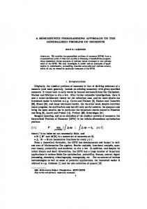
6.1. 2-Bar Truss Consider a two-bar truss illustrated in Fig.1 (a). The nodes (b) and (c) are pin-supported at (x, y) = (0, 100.0) and (0, 0) in cm, respectively, while the node (a) is free, i.e., nd = nm = 2. The nominal external load � f = (98.0, 0) kN is applied at the node (a). Consider the stress constraints of all members defined by (7) with σci = −σci = 98.0 MPa, i = 1, 2. The initial solution a0 for Algorithm 4.1 is given as a0 = (20.0, 40.0) cm2 . Based on Propo26
sition 3.1, we solve the SDP problem (17) by using the primal-dual interior-point method to find � α(a0 ) = 69.297 kN. The maximization problem (24) of robustness function is solved by using Algorithm 4.1. The upper bound of structural volume is given as V = 76.5685 cm3 so that the volume constraint becomes active at a = a0 , i.e., V = V(a0 ). We choose ck = 10−5 at each iteration of Algorithm 4.1, and set � = 0.05. The iteration history is listed in Table 1. The obtained optimal cross-sectional areas are a∗ = (32.1895, 31.3807) cm2 . The corresponding robustness function is � α(a∗ ) = 153.766 kN. In order to verify these results, we randomly generate a number of ζ, and compute the corresponding member stresses σi . For the initial solution a0 , Fig.1 (b) shows the obtained stress states (σ1 /σ1 , σ2 /σ2 ) corresponding to randomly generated ζ ∈ Z(� α(a0 )). From Fig.1 (b) it is observed that the stress constraints (7) are satisfied for all generated ζ. The worst case corresponds to ζ = (49.0, −49.0) kN, where the constraint σ1 ≤ σ1 becomes active. For the optimal solution a∗ , Fig.1 (c) shows (σ1 /σ1 , σ2/σ2 ) computed from randomly generated ζ ∈ Z(� α(a∗ )). From Fig.1 (c) it is seen that the constraints (7) are always satisfied, and the constraints σ1 ≤ σ1 , σ2 ≤ σ2 and σ2 ≥ σ2 become active in the worst cases, i.e., the constraints on both members can happen to be active.
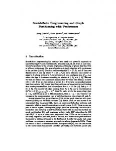
6.2. 29-Bar Truss Consider a truss illustrated in Fig.2 (a). The nodes (a) and (b) are pin-supported at (x, y) = (0, 100.0) and (0, 0) in cm, respectively, where nd = 20 and nm = 29. The lengths of members in the x- and y-directions are 50.0 cm. As the nominal external forces � f , (0, −9.8) kN are applied at 27
d
the nodes (c) and (d). The uncertainty set of f is defined by (9) and (10) with ζ ∈ Rn and Γ = I. Hence, uncertain loads can possibly exist at all nodes. The stress constraints (7) are considered for all members with σi = −σi = 4.9 × 10² MPa, i = 1, . . . , nm , and nc = nm . The maximization problem (24) of robustness function is solved by using Algorithm 4.1. In Algorithm 4.1, we set a0i = 20.0 cm2 , i = 1, . . . , nm , � = 0.1, ck = 10−5 , ∀k, and V = V(a0 ) = 3.3971 × 104 cm3 . The robustness function at the initial solution a = a0 is computed as � α(a0 ) = 0.71161 kN by solving Problem (17). The optimal design a∗ computed by Algorithm 4.1 after 53 iterations is shown in Fig.2 (b). The α(a∗ ) = 10.8496 kN. As discussed in Remark 4.2, we solve Probrobustness function at a = a∗ is � lem (25) in Step 2 of Algorithm 4.1 by converting it to Problem (31), where the number of variables 60 2 21 29 is y ∈ R61 and the dimension of constraints is K = R59 + × L+ × S+ × (S+ ) . The average and
standard deviation of CPU time required to solve Problem (31) are 7.80 sec and 1.21 sec, respectively. Similarly, in Step 1, Problem (17) is converted to the form of Problem (30) with y ∈ R30 and 21 29 K = R29 + × (S+ ) . Some software packages for SDP, including SeDuMi, incorporate efficient meth-
ods for computation when the coefficient matrix A of Problem (30) is sparse; e.g., see (Ref. 27). Note that Di , i = 0, 1, . . . , nm , in Problem (31) are sparse because ∂K(ak )/∂ai , i = 1, . . . , nm , are usually very sparse matrices. For stress constraints, Hl , l = 1, . . . , nc , are also sparse. Hence, Problem (31) have sparse coefficient matrices. Figs.2 (c) and (d) show σi /σi with a = a0 and a = a∗ , respectively, corresponding to randomly 28
generated ζ ∈ Z(� α(a0 )) and ζ ∈ Z(� α(a∗ )). It is observed from Fig.2 (c) that the worst cases at a = a0 corresponds to ζ such that the constraints σ9 ≤ σ9 and/or σ15 ≥ σ15 become active. On the other hand, from Fig.2 (d), we can see that the stress constraints (7) of almost all members happen to become active at a = a∗ . Note that the actual worst-case behaviors cannot be exactly predicted, in general, by taking a rather small number of random samples of ζ.
7. Conclusions In this paper, based on the robustness function (Ref. 13), we have proposed a novel concept as well as a global convergent algorithm for the robust structural optimization. We assume that the constraints on mechanical performance can be expressed by using some polynomial inequalities. It has been shown that the robustness function of a linear elastic structure submitted to uncertain loads can be obtained by solving the linear semidefinite programming (SDP) problem. As a scheme of the robust structural optimization, we have introduced the maximization problem of robustness function, which has been formulated as a nonlinear SDP problem. A sequential SDP approach has been presented, in which SDP problems are successively solved by the primal-dual interior-point method to obtain the optimal truss designs. The method has been shown to be globally convergent under certain assumptions. In the numerical examples of various structures, we have illustrated that the optimal truss designs can be found without any difficulty by our algorithm. Besides the computational efficiency, the pro-
29
posed algorithm has the advantage such that, at each iteration of the algorithm, the SDP problems can be solved by using the well-developed softwares based on the primal-dual interior-point method. Therefore, our major task is limited to input the constant matrices and vectors defining the SDP problems and no effort is required to develop any optimization software.
References
1. Tsompanakis, Y., and Papadrakakis, M., Large-Scale Reliability-Based Structural Optimization, Structural and Multidisciplinary Optimization, Vol. 26, pp. 429–440, 2004.
2. Kharmanda, G., Olhoff, N., Mohamed, A., and Lemaire, M., Reliability-Based Topology Optimization, Structural and Multidisciplinary Optimization, Vol. 26, pp. 295–307, 2004.
3. Choi, K.K., Tu, J., and Park, Y.H., Extensions of Design Potential Concept for Reliability-Based Design Optimization to Nonsmooth and Extreme Cases, Structural and Multidisciplinary Optimization, Vol. 22, pp. 335–350, 2001.
4. Jung, D.H., and Lee, B.C., Development of a Simple and Efficient Method for Robust Optimization, International Journal for Numerical Methods in Engineering, Vol. 53, pp. 2201–2215, 2002.
5. Doltsinis, I., and Kang, Z., Robust Design of Structures Using Optimization Methods, Computer Methods in Applied Mechanics and Engineering, Vol. 193, pp. 2221–2237, 2004.
30
6. Ben-Haim, Y., and Elishakoff, I., Convex Models of Uncertainty in Applied Mechanics, Elsevier, New York, New York, 1990.
7. Pantelides, C.P., and Ganzerli, S., Design of Trusses under Uncertain Loads using Convex Models, Journal of Structural Engineering, ASCE, Vol. 124, pp. 318–329, 1998.
8. Ben-Tal, A., and Nemirovski, A., Robust Optimization: Methodology and Applications, Mathematical Programming, Vol. 92B, pp. 453–480, 2002.
9. Ben-Tal, A., and Nemirovski, A., Robust Truss Topology Optimization via Semidefinite Programming, SIAM Journal on Optimization, Vol. 7, pp. 991–1016, 1997.
10. Koˇcvara, M., Zowe, J., and Nemirovski, A., Cascading: An Approach to Robust Material Optimization, Computers & Structures, Vol. 76, pp. 431–442, 2000.
11. Han, J.S., and Kwak, B.M., Robust Optimization using a Gradient Index: MEMS Applications, Structural and Multidisciplinary Optimization, Vol. 27, pp. 469–478, 2004.
12. Calafiore, G., and El Ghaoui, L., Ellipsoidal Bounds for Uncertain Linear Equations and Dynamical Systems, Automatica, Vol. 40, pp. 773–787, 2004.
13. Ben-Haim, Y., Information-Gap Decision Theory, Academic Press, London, UK, 2001.
14. Kanno, Y., and Takewaki, I., Robustness Analysis of Trusses with Separable Load and Structural Uncertainties, International Journal of Solids and Structures (to appear). 31
15. Wolkowicz, H., Saigal, R., and Vandenberghe, L., Editors, Handbook of Semidefinite Programming: Theory, Algorithms, and Applications, Kluwer Academic Publishers, Dordrecht, Netherlands, 2000.
16. Jarre, F., Some Aspects of Nonlinear Semidefinite Programming, System Modeling and Optimization: IFIP 20th Conference on System Modeling and Optimization, Edited by E.W. Sachs and R. Tichatschke, Kluwer Academic Publishers, Dordrecht, Netherlands, pp. 55–69, 2003.
17. Fukushima, M., Takazawa, K., Ohsaki, S., and Ibaraki, T., Successive Linearization Methods for Large-Scale Nonlinear Programming Problems, Japan Journal of Industrial and Applied Mathematics, Vol. 9, pp. 117–132, 1992.
18. Kanzow, C., Nagel, C., Kato, H., and Fukushima, M., Successive Linearization Methods for Nonlinear Semidefinite Programs, Computational Optimization and Applications, Vol. 31, pp. 251–273, 2005.
19. Kojima, M., and Tunc¸ el, L., Cones of Matrices and Successive Convex Relaxations of Nonconvex Sets, SIAM Journal on Optimization, Vol. 10, pp. 750–778, 2000.
20. Simo, J.C., and Hughes, T.J.R., Computational Inelasticity, Springer-Verlag, New York, New York, 1998.
32
21. Ben-Tal, A., and Nemirovski, A., Lectures on Modern Convex Optimization: Analysis, Algorithms, and Engineering Applications, SIAM, Philadelphia, Pennysylvania, 2001.
22. Ohsaki, M., Fujisawa, K., Katoh, N., and Kanno, Y., Semidefinite Programming for Topology Optimization of Truss under Multiple Eigenvalue Constraints, Computer Methods in Applied Mechanics and Engineering, Vol. 180, pp. 203–217, 1999.
23. Kanno, Y., Ohsaki, M., and Katoh, N., Sequential Semidefinite Programming for Optimization of Framed Structures under Multimodal Buckling Constraints, International Journal of Structural Stability and Dynamics, Vol. 1, pp. 585–602, 2001.
24. Sturm, J.F., Using SeDuMi 1.02, a MATLAB Toolbox for Optimization over Symmetric Cones, Optimization Methods and Software, Vol. 11/12, pp. 625–653, 1999.
25. The MathWorks, Using MATLAB, The MathWorks, Natick, Massachusetts, 2002.
26. Kanno, Y., and Takewaki, I., Sequential Semidefinite Program for Maximum Robustness Design of Structures under Load Uncertainties, Kyoto University, BGE Research Report 04-05, July 2004 (revised: July 2005); availabe at http://www.archi.kyoto-u.ac.jp/˜bge/RR/.
27. Fujisawa, K., Kojima, M., and Nakata, K., Exploiting Sparsity in Primal-Dual Interior-Point Methods for Semidefinite Programming, Mathematical Programming, Vol. 79, pp. 235–253, 1997.
33
y (a)
(1)
∼f
(b)
(2)
x
0 (c)
1
1
0.8
0.8
0.6
0.6
0.4
0.4
0.2
0.2
σ2 /⎯σ2
σ2 /⎯σ2
(a) model
0 −0.2
0 −0.2
−0.4
−0.4
−0.6
−0.6
−0.8
−0.8
−1 −0.4
−1 −0.2
0
0.2
0.4 σ 1 /⎯σ1
0.6
0.8
1
−0.4
−0.2
0
0.2
0.4 σ 1 /⎯σ1
0.6
0.8
1
(c) at a = a∗ with α = 153.766 kN
(b) at a = a0 with α = 69.297 kN
Figure 1: 2-Bar Truss Example: Model definition and stress states at the initial and optimal designs for randomly generated ζ ∈ Z(α).
34
y (a)
(10)
(9) (18)
(1)
(15)
0
(14)
(22) (4)
(23) (6)
(28)
(7)
(26)
(13)
(21) (27)
(5)
(25)
(12)
(2)
(20)
(19) (3)
(24)
(11)
(8)
(29) (17)
(16) (c)
(b)
(d)
x
∼f
∼f
(a) model
(b) optimal design
1 0.8 0.6 0.2
σi /⎯σi
σi /⎯σi
0.4 0 −0.2 −0.4 −0.6 −0.8 −1 0
5
10
15 20 members (i)
25
30
(d) at a = a∗ with α = 10.8496 kN
(c) at a = a0 with α = 0.71161 kN
Figure 2: 29-Bar Truss example: Model definition, optimal design, and stress states at the initial and optimal designs for randomly generated ζ ∈ Z(α).
35
Table 1: Iteration history of optimization of the 2-bar truss by Algorithm 4.1. k � αk = (tk )1/2 (kN) 0 69.297 1 105.821 2 147.520 3 153.750 4 153.766
ak1 (cm2 ) 20.0000 25.2708 31.2883 32.1938 32.1895
36
ak2 (cm2 ) 40.0000 36.2730 32.0180 31.3777 31.3807
�∆xk �2 59.7803 92.4996 30.1372 1.6035 0.0167