Sequential spatial reasoning in images based on pre-attention mechanisms and fuzzy attribute graphs Geoffroy Fouquier1 and Jamal Atif2 and Isabelle Bloch1 Abstract. Spatial relations play a crucial role in model-based image recognition and interpretation due to their stability compared to many other image appearance characteristics, and graphs are well adapted to represent such information. Sequential methods for knowledgebased recognition of structures require to define in which order the structures have to be recognized, which can be expressed as the optimization of a path in the representation graph. We propose to integrate pre-attention mechanisms in the optimization criterion, in the form of a saliency map, by reasoning on the saliency of spatial area defined by spatial relations. Such mechanisms extract knowledge from an image without object recognition in advance and do not require any a priori knowledge on the image. Therefore, pre-attentional mechanisms provide useful knowledge for object segmentation and recognition. The derived algorithms are applied on brain image understanding.
1 Introduction Sequential segmentation is a useful approach for knowledge-based object recognition where objects are segmented in a predefined order, starting from the simplest object to segment to the most difficult one. The segmentation and recognition of each object is then based on a generic model of the scene and relies on the previously recognized objects. This approach, as developed e.g. in [3], requires to define the order according to which the objects have to be recognized and the choice of the most appropriate order is one of the difficulties raised by this approach. Here, the recognition and the segmentation of the objects of the scene are performed at the same time. The sequence of objects may be expressed as a path in a graph, where each node of the graph represents an object. In this paper, we propose a new approach to this problem integrating information extracted from the data, based on the notion of saliency. The visual system is usually modeled using pre-attentional and attentional mechanisms. Basically, the purpose of the pre-attentional step is to guide the attentional step to select salient parts in the scene. This selection allows the attentional process to focus only on the salient part (object or region) and thus reduces the computational cost of this mechanism. We can easily draw some similarities between the iterative segmentation scheme and the visual system: the pre-attentional mechanism could correspond to the selection of the next object to segment and the attentional mechanism to the segmentation of an object of the scene (and its interpretation). Thus the iterative segmentation framework is viewed as a scene exploration and analysis process. 1 2
TELECOM ParisTech (ENST), CNRS-LTCI UMR 5141, Paris, France {geoffroy.fouquier, isabelle.bloch}@enst.fr IRD-Cayenne/UAG, email:
[email protected]
Our contribution is to introduce a pre-attentional mechanism in the optimization of the segmentation path for a sequential image segmentation process. This article is organized as follows. First we present in Section 2 how to represent the knowledge composing the generic model of the scene. In Section 3, a brief overview of the modeling of the visual system is given as well as a presentation of the pre-attentional mechanism used in the following section. Then we present in Section 4 a way to evaluate which information is given by the attentional mechanism. Then, Section 5 presents a way to integrate the saliency map into the segmentation process. Experiments and results are presented in Section 6 on an example of brain image understanding and Section 7 draws some conclusions.
2 Knowledge representation Graphs are well adapted to represent generic knowledge, such as spatial relations between the objects of a scene. In the sequential segmentation framework, the generic model of the scene is modeled as a graph where each vertex represents an object of the scene and each edge represents one or more spatial relations between two objects. We introduce the following notations: Let ΣV , ΣE be the sets of vertex labels and edge labels, respectively. Let V be a finite nonempty set of vertices, Lv be a vertex interpreter Lv : V → ΣV , E be a set of ordered pairs of vertices called edges, and Le be an edge interpreter Le : E → ΣE . Then G = (V, Lv , E, Le ) is a labeled graph with directed edges. For v ∈ V and e ∈ V ×V , δ(v, e) is a transition function that returns the vertex v ′ such that e = (v, v ′ ). For v ∈ V , A(v) returns the set of edges adjacent to v. Finally, p = (v1 , v2 , ..., vn ) is a path of length n labeled as lp = (v1 , e(v1 , v2 ), v2 , ..., vn ). A knowledge base KB defines all the spatial relations existing between vertices in the graph: KB = {vi Rvj , vi , vj ∈ V, R ∈ R} and e = (v1 , v2 ) ∈ E ⇐⇒ ∃R ∈ R, (v1 Rv2 ) ∈ KB, where R is the set of relations. In the following, we use fuzzy representations of the spatial relations, since they are appropriate to model the intrinsic imprecision of several relations (such as “close to”, “behind”, etc.), the potential variability (even if it is reduced in normal cases) and the necessary flexibility for spatial reasoning [2]. Here, the representation of a spatial relation is computed as the region of space in which the relation R to an object A is satisfied. The membership degree of each point corresponds to the satisfaction degree of the relation at this point. Figure 2 (b,c) presents an example of a structure and the region of space corresponding to the region “to the right of” this structure. A directed edge between two vertices v1 and v2 carries at least one spatial relation between these objects. An edge interpretor associates to each edge a fuzzy set µRel , defined in the spatial domain S,
representing the conjunctive merging of all the representations of the spatial relations carried by this edge to a reference structure. Since there is at least one spatial relation carried by an edge, µRel cannot be empty. Let µeRi , i = 1, ..., ne the ne relations carried by an edge e. Then µeRel is expressed as: µeRel = ⊤i=1..ne (µeRi ) with ⊤ a t-norm (fuzzy conjunction) [4]. Since objects are sequentially segmented, we propose to focus our attention by using known spatial relations with previously segmented objects. The set of target objects is filtered as the set of unsegmented objects which have a spatial relation with a previously segmented object. The set of segmented objects is filtered likewise as the set of objects which have a spatial relation with an unsegmented object of interest. The “search area” is thus defined by the merging of the representations of known spatial relations between previously segmented objects which have an edge in the graph with the target object. We now describe the modeling of the main relations that we use: distances and directional relative positions. A distance relation can be defined as a fuzzy interval f of trapezoidal shape on R+ . A fuzzy subset µd of the image space S can then be derived by combining f with a distance map dA to the reference object A: ∀x ∈ S, µd (x) = f (dA (x)), where dA (x) = inf y∈A d(x, y). The relation “close to” can be defined as a function of the distance between two sets: µclose (A, B) = h(d(A, B)) where d(A, B) denotes the minimal distance between points of A and B: d(A, B) = inf x∈A,y∈B d(x, y), and h is a decreasing function of d, from R+ into [0, 1]. We assume that A ∩ B = ∅. The relation of adjacency can be defined likewise as a “very close to” relation, leading to a degree of adjacency instead of a Boolean value, making it more robust to small errors. Directional relations are represented using the “fuzzy landscape approach” [1]. A morphological dilation δνα by a fuzzy structuring element να representing the semantics of the relation “in direction α” is applied to the reference object A: µα = δνα (A), where να is defined, for x in S given in polar coordinates (ρ, θ), as: να (x) = g(|θ − α|), where g is a decreasing function from [0, π] to [0, 1], and |θ − α| is defined modulo π. This definition extends to 3D by using two angles to define a direction. The example in Figure 2 (b,c) has been obtained using this definition. Other relations can be modeled in a similar way [2]. These models are generic, but the membership functions depend on a few parameters that have to be tuned for each application domain according to the semantics of the relations in that domain.
3 Saliency Maps Among the pre-attentional mechanisms, we focus on the saliency map, as defined by Koch and Ullman [6]. This mechanism allows selecting areas using some basic features easily computable on every type of images. Figure 2 presents a saliency map and its restriction around an object which allows exploring the area of the image around the object. This approach uses three basic features: intensity, color and orientation. For each feature, the difference between a location and its immediate surrounding is computed. For intensity, this is the difference of contrast. For color, two oppositions of colors are studied: between red and green on the one hand, and between blue and yellow on the other and. And for orientation, four directions are studied with Gabor filters. Overall, seven features are considered. Nine scale spaces are created with dyadic Gaussian pyramids for each feature and six maps are derived by center-surround difference between the fine scale c in {2, 3, 4} and the coarse scale of the pyramid
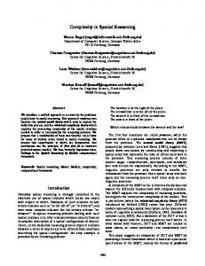
s = c+d, with d in {3, 4}. Finally, all maps corresponding to a same feature are normalized, and a conspicuity map per feature (the sum of all corresponding maps) is computed. Then the three conspicuity maps are merged with a weighted mean to produce the saliency map. Figure 1 presents an example of a saliency map.
Figure 1. Lena and the corresponding saliency map (dark: not
salient, bright: most salient parts) This approach is a data-driven bottom-up approach, and the only top-bottom connections is for the occlusion of the most salient location. But more top-bottom connections are required to define protoobjects [7], an extension of the first method recently presented. In this case, the saliency map is computed as in the original method, but once the most salient location is detected, a feedback connection allows finding which conspicuity map, and then which map produces this salient location (or contributes the most). Then, a proto-object is defined as the connected component (a pixel belongs to the component if one of its neighbors is in the component, and if its value is higher than a threshold) at the same location of the higher value of the saliency map, on the map which produces it.
4 Evaluating saliency on manually segmented structures The sequential segmentation framework with the optimized segmentation path described in [5] uses generic knowledge and a segmented database and therefore cannot take into account the intrinsic segmentation difficulties of each object. These difficulties vary with respect to the object features: shape, homogeneity, texture or boundaries, or image noise. Some generic rules could be constructed, e.g. this object is more difficult to segment than this other one, but this kind of rule is not necessarily true for each image even in a restricted application domain. We consider that the information of saliency is directly related to the difficulties of segmentation because an object with a salient border will be much simpler to segment than an object with a less salient border. Therefore, we propose a methodology to derive the difficulty of segmentation from saliency information and to compare all the areas of saliency corresponding to the previously segmented objects. The area of saliency for an object corresponds to the saliency map masked by the segmentation (a binary map) of this object and possibly its surrounding. Depending on the class of segmentation algorithms, we may not be interested by the same parts of the objects. If we consider an edgebased segmentation algorithm, then we consider that the most important area to take into account for the image segmentation is the border of the object. In this case, the interesting part of the object should be extracted for example as the dilated segmentation of the object, in order take into account the surrounding of the border. In a region-based segmentation, the whole object is extracted depending on a homogeneity criterion. The saliency map is masked, in this case, by the extracted object.
(a)
(b)
(c)
(d)
(e)
Figure 2. (a) A slice of a 3D Magnetic Resonance Image. (b) Right lateral ventricle. (c) Fuzzy subset corresponding to the spatial relation
“right of” (b). (d) A slice of the saliency map of (a). (e) Saliency around the ventricle (dark: not salient, bright: most salient parts) Once the saliency for the surrounding of each object has been extracted, an histogram of the saliency map is computed for each object. Once normalized, we have a distribution of the saliency for each object. Therefore, we propose to estimate the difficulty of segmentation as a comparison of the histograms of saliency. In our experiments, we compute the energy of the histogram as a criterion of comparison between histograms. The energy of the histogram H, with N P 2 bins, is computed as follows: energy(H) = N h(n) where h is the function that counts the number of occurrences of value n in the saliency map. Figure 5 presents two histograms of several objects from two images. This methodology is not used for a segmentation purpose (here we are trying to get rid of the usage of a previously segmented base), but only to study the saliency of the different objects and to exhibit the potential interest of this type of measure.
5 Using saliency for image interpretation Approaches relying on the shape of the target object, like in [5], make the assertion that the generic model is always valid, i.e. that all objects from the generic model are always present and no new object can be taken into account. Here, the exploration relies on the previously recognized objects only and not on the shape of the target object, which allows dealing with changes in the model. Image segmentation is seen as a scene exploration process, where only a small region of space is analyzed at a given time, i.e. objects are segmented individually. Also, the exploration of a new area of space uses the previously explored area, here the segmented objects are used to segment the remaining parts of the scene. The process is guided using a pre-attentional mechanism, here a saliency map, which indicates the most salient area of space in the search domain. This area is computed using the already known part of the scene and the spatial relations existing between these objects and the objects that still to be found. Figure 3 presents the general scheme of the method. At first, we present how the graph is filtered to compute the area of search, then we present the process of selecting the next object to segment. In the following, the original image is denoted by I. The vertices of the graph are divided into two disjoint groups of vertices: V = Vseg ∪ Vtar . At the beginning of the process, a first object is considered as known and segmented: Vseg = {vinit }. This object can be detected using saliency in the image, or other information (in brain imaging, the lateral ventricle can be segmented using a completely different scheme for example). The recognition of an object implies thus to move a vertex from the set of target vertices to the set of segmented vertices and it is mandatory that the vertex to segment is directly connected to the set of already segmented vertices. An iteration of the sequential segmentation is expressed as a function of the previously segmented objects Vseg , the chosen next object to segment vˆ, the saliency map of the image salI , the original image I and Ef the spatial relations between both sets of objects, already segmented and to be segmented,
respectively: i i−1 Vseg = seqseg(Vseg , vˆ, salI , I, Efi−1 )
where the superscript i denotes the iteration. Accordingly the set of target vertices is filtered so as to keep only the vertices connected with the already segmented set of vertices. Likewise, the latter set is filtered to the subset of vertices connected with an edge to the set of target objects. The set of edges is filtered accordingly. The obtained subgraph forms a bipartite graph composed by both sets of known and target objects, and by the set of edges representing the spatial relations between both groups of vertices: Vf s = {v1 ∈ Vseg | ∃v2 ∈ Vtar , (v1 , v2 ) ∈ E} Vf t = {v2 ∈ Vtar | ∃v1 ∈ Vseg , (v1 , v2 ) ∈ E} Ef = {(vt , vs ) | vt ∈ Vf t , vs ∈ Vf s } For each edge e in Ef , the edge interpretor produces µeRel . The area of space of the search domain is defined as the merging of the support of all edge representations, given by the edge interpretor: µsd = ⊥e∈Ef (µeRel ) with ⊥ a t-conorm (fuzzy disjunction) [4]. The binary map corresponding to the search domain gives an area of space which includes the spatial location of all the target objects (hence a disjunction combination). Note that this spatial location could cover a large part of the image space, particularly if the only spatial relation between two objects is a relation of direction. The search domain sd is simply defined as: sd = support(µsd ) Now, we present how the process of selection of a target vertex by an analysis of the saliency in the search domain. The filtering of the graph gives two groups of vertices: Vf s and Vf t and we have to choose in Vf t the next vertex (and so the object that the vertex represents) to recognize. For each candidate vertex v, its estimated spatial location is defined by the merging of the spatial relations connecting this vertex to the previously recognized vertices: locv = ⊤e∈(A(v)∩Ef ) (µeRel ) with ⊤ a t-norm. This estimated spatial location of a vertex is then combined with the search domain, to extract the saliency in the area of the estimated location of the target object and its surrounding: saliencyv = ⊤(locv , sd, salI ) An histogram of this area is then produced. We select the next object to segment by an analysis of this histogram. Among other measures, the energy of the histogram (previously defined) is kept as a criterion of selection and allows selecting the most salient area and then the next object to segment: vˆ = arg max (energy(Hv )) v∈Vft
Generic Knowledge
:already segmented : to be segmented
original image saliency map
2 1 4 Model Graph
3
2 1
2
3
1
search domain Saliency around 3
3
Structure Selection
Saliency around 4
4 Filtered fuzzy subsets graph representing spatial relations
4 current graph 2
3
1 updated graph
Segmentation 4
Figure 3. Block diagram of the proposed method to include a pre-attentional mechanism into sequential segmentation.
the exploration of the scene consists then in moving a vertex from the set of target vertices to the set of known vertices, and the selection of the moved vertex is realized by the comparison of the saliency of each object area of the search domain, which corresponds to a modeldriven exploration of the scene. This method allows us to directly take into account the knowledge given by the current image and does not rely on a representation of the target objects during the process. The segmentation of the object is expressed as a function of the selected object to segment vˆ, selected with a criterion based on saliency, its spatial relations with the previously segmented objects and the original image: segvˆ = segment(ˆ v, locvˆ , I) Finally, the set of segmented object is updated: i−1 i i−1 i Vseg = Vseg ∪ {ˆ v } and Vtarget = Vtarget \ {ˆ v}
Finally, 9 maps are extracted. Note that we could extract more planes allowing to take into account more directions thus better isotropy. Experiments have been conducted using a manually segmented database of human brain 3D MRI (IBSR database). This database is composed by 18 brain images with their segmentations. The parameters of the membership functions used to computed the representation of the spatial relations are learned on a database of healthy cases (IBSR) and pathological cases (5 differents cases so far, corresponding to different types of brain tumor). Table 1 presents some relations used in our experiments. Table 1. Some relations used in our experiments. LLV: left lateral ventricle LCN: left caudate nucleus, LTH: left thalamus and LPU: left Putamen. v1 LLV LLV LLV LCN LCN
R RightOf CloseTo DownOf RightOf InFrontOf
v2 LCN LCN LTH LPU LTH
v1 LCN LTH LTH LTH
R UpOf BehindOf DownOf RightOf
v2 LTH LCN LCN LPU
6 Application to human brain structures recognition Saliency map on 3-dimensions MRI Saliency maps, especially according to Koch and Ullman, are usually computed on 2D natural images with a sufficient resolution to produce the requested scale of the dyadic pyramid. In the case of 3D magnetic resonance images (MRI), the resolution of the image is often small. The IBSR database3 images used during our experiments have the following size: 256 × 256 × 128. We limit our pyramid to 7 scales (including the original scale). The fine scale used to compute maps are 1, 2 and 3. The coarse scale are the fine scale plus a δ ∈ {2, 3}, i.e. 1 + 2, 1 + 3, 2 + 2, 2 + 3, . . . . Finally, the saliency map is computed with the size of the third level of the dyadic pyramid. 3D MRI provides only one channel which is considered as an intensity in the computation. Since there is no color channel, color features are just removed. For orientation, we use a similar approach as in 2 dimensions, but on 3 different planes defined by the axis x and y for the first plane, x and z for the second, y and z for the last one. We considered 4 directions for each plane and removed the duplicates. 3
Internet Brain Segmentation Repository. The MR brain data sets and their manual segmentations were provided by the Center for Morphometric Analysis at Massachusetts General Hospital and are available at http://www.cma.mgh.harvard.edu/ibsr/
Saliency on manually segmented structures In our experiments, the area of saliency taken into account for each structure corresponds to the 3D binary map of the segmentation of one object dilated by a elementary structuring element in 6-connectivity. The saliency map is normalized between 0 and 255. The histogram in Figure 4 presents the saliency for each of the three structures on all images, and it shows the variation of saliency, although the IBSR data set is quite uniform. This variation shows that the measure of saliency takes into account specific information about each image. Table 2 presents saliency measures for three anatomical structures of the human brain plus the same measure for the white matter and the gray matter. These measures (energy of the histogram) are always higher for the three anatomical structures. Figure 5 presents some histograms of saliency for these structures. Histograms of saliency for gray and white matter are in most of the cases larger and lower than histograms for other structures, and particularly the histograms of caudate nucleus and putamen. Thus, there is more saliency in the area of the anatomical structures than in areas of gray or white matter, which does not present much information. Comparing structures, it appears that the thalamus has generally lower values (it has less well defined boundaries). Hence it can be expected that its segmentation
0.2
Table 2. Saliency measures (energy measure of saliency histogram)
for 3 anatomical structures, white matter (LWM) and gray matter (LGM) for all images of the IBSR database. LCN: left caudate nucleus, LTH: left thalamus and LPU: left Putamen. LCN 0.065 0.097 0.039 0.050 0.038 0.054 0.039 0.040 0.039 0.045 0.037 0.033 0.037 0.046 0.033 0.032 0.045
LTH 0.057 0.064 0.033 0.031 0.028 0.038 0.024 0.026 0.026 0.030 0.025 0.029 0.033 0.030 0.026 0.025 0.032
LPU 0.068 0.095 0.042 0.054 0.107 0.099 0.046 0.046 0.061 0.060 0.048 0.032 0.069 0.061 0.044 0.044 0.049
LWM 0.026 0.041 0.027 0.026 0.027 0.038 0.023 0.020 0.026 0.027 0.019 0.026 0.031 0.025 0.017 0.022 0.022
LGM 0.015 0.020 0.017 0.017 0.018 0.025 0.018 0.014 0.020 0.014 0.011 0.017 0.020 0.017 0.014 0.015 0.020
will be more difficult. 0.03 Ventricle CaudateNucleus Putamen Thalamus
0.025
0.02
0.015
0.01
0.005
0
0
50
100
150
200
250
300
Figure 4. The histograms of the saliency of each structure for all
images in the database. Sequential segmentation Starting from the lateral ventricle, we are looking for the next structure to segment. Table 3 presents the measures of saliency for the two structures connected to the lateral ventricle in the graph, the caudate nucleus and the thalamus, and the same measure, after the segmentation of the first structure. For all the images of the IBSR database, the same path is selected but with some variation of the criterion values. The resulting path corresponds to the path used in [3], defined intuitively, in a supervised way, thus with visual hints. It is hence very satisfactory to find the same path automatically using a saliency feature. The IBSR base is also a quite homogeneous database, and all images have been registered, lowering the difference between the images. Experiments on images with a higher variability, including pathological ones, are currently conducted. Figure 6 presents a typical segmentation using the resulting path.
Ventricle CaudateNucleus Putamen Thalamus White Matter Gray Matter
0.18
0.16
LLV LCN LPU LTH LLV LWM LGM
0.14
0.12
0.1
0.08
0.06
0.04
0.02
0
IBSR 02
0
20
40
60
80
100
120
140
160
180
200
hist. IBSR 02
Figure 5. Histograms of saliency for 4 anatomical structures, white
matter and gray matter of the left hemisphere in a 3D MRI. In this case, the saliency is high for all structures, ventricle and caudate saliency histograms are clearly distinct from putamen and thalamus ones. Saliency of white matter and gray matter are lower than saliency of internal structures. Table 3. Measure of saliency for two successive selections, for each image in the IBSR database. The initial structure is the left lateral ventricle 1st selection LLV → LCN LTH 0.035 0.016 0.048 0.023 0.018 0.011 0.018 0.011 0.017 0.011 0.022 0.013 0.017 0.011 0.016 0.011 0.021 0.014 0.018 0.013 0.017 0.010 0.017 0.010 0.019 0.012 0.017 0.011 0.017 0.010 0.014 0.010 0.019 0.014
2nd selection (LCN,LLV) → LTH LPU 0.015 0.012 0.022 0.017 0.011 0.009 0.011 0.010 0.011 0.009 0.013 0.012 0.011 0.010 0.011 0.010 0.014 0.013 0.012 0.010 0.010 0.009 0.010 0.009 0.012 0.011 0.010 0.009 0.010 0.009 0.010 0.010 0.014 0.013
[2] I. Bloch, ‘Fuzzy Spatial Relationships for Image Processing and Interpretation: A Review’, Image and Vision Computing, 23(2), 89–110, (2005). [3] O. Colliot, O. Camara, and I. Bloch, ‘Integration of Fuzzy Spatial Relations in Deformable Models - Application to Brain MRI Segmentation’, Pattern Recognition, 39, 1401–1414, (2006). [4] D. Dubois and H. Prade, Fuzzy Sets and Systems: Theory and Applications, Academic Press, New-York, 1980. [5] G. Fouquier, J. Atif, and I. Bloch, ‘Local Reasoning in Fuzzy Attributes Graphs for Optimizing Sequential Segmentation’, in 6th IAPRTC15 Workshop on Graph-based Representations in Pattern Recognition, GbR’07, ed., springer, volume 4538 of LNCS, pp. 138–147, Alicante, Spain, (Jun 2007). [6] L. Itti, C. Koch, and E. Niebur, ‘A model of saliency-based visual attention for rapid scene analysis’, IEEE Transactions on Pattern Analysis and Machine Intelligence, 20(11), 1254–1259, (Nov. 1998). [7] D. Walther and C. Koch, ‘Modeling attention to salient proto-objects’, Neural Networks, 19(9), 1395–1407, (Nov. 2006).
7 Conclusion We have presented a sequential segmentation framework viewed as a scene exploration process, and guided by a pre-attentional mechanism, here saliency map. Preliminary results show that saliency provides intrinsic information about the image, usable for its segmentation. Further work will be done on a larger graph with more structures and relations between them.
REFERENCES [1] I. Bloch, ‘Fuzzy Relative Position between Objects in Image Processing: a Morphological Approach’, IEEE Transactions on Pattern Analysis and Machine Intelligence, 21(7), 657–664, (1999).
Figure 6. Typical segmentation using the path found in our experiments