network size. Our solution is based on a mathematical model that characterizes performance accurately without extensive simulations. SERAN is robust against ...
1
SERAN: A Semi Random Protocol Solution for Clustered Wireless Sensor Networks † A. Bonivento, ‡ C. Fischione ∗ , † A. Sangiovanni-Vincentelli, ‡ F. Graziosi, ‡ F. Santucci † U.C. Berkeley, ‡ University of L’Aquila (Italy) e-mail: † (alvise,alberto)@eecs.berkeley.edu, ‡ (fischione, graziosi, santucci)@ing.univaq.it
Abstract— SERAN is a two-layer (routing and MAC) protocol for wireless sensor networks in manufacturing plants. At both layers, SERAN combines a randomized and a deterministic approach. While the randomized component provides robustness over unreliable channels, the deterministic component avoids an explosion of packet collisions and allows our protocol to scale with network size. Our solution is based on a mathematical model that characterizes performance accurately without extensive simulations. SERAN is robust against node failures and clock drifts, supports data aggregation algorithms and is easily implementable in any of the existing hardware platforms. Although SERAN was designed for manufacturing plants applications, it can be used in any type of clustered topology. We consider a representative case study and we present simulation results to show SERAN efficiency.
I. I NTRODUCTION Although wireless technology experienced great advancements in the last years, very little of this revolution touched the world of industrial automation. Most of the control application within manufacturing plants are currently running on cable-based communication infrastructures with obvious disadvantages on maintenance and deployment costs. The main reason for the delay in the adoption of wireless sensor networks within manufacturing plants is the lack of protocols that address both network and MAC layers, and that are able to guarantee latency and quality of service under unreliable channel conditions. Most of the applications developed for wireless sensor networks are concerned with outdoor environmental monitoring. Those results can be hardly extended to the manufacturing plant domain where the presence of a large amount of moving metal objects makes robustness a first level priority for protocol design. Furthermore, most of the existing approaches deal with single layer protocols, without a clear indication of how these fit in an overall solution. Particularly, it is not always clear what are the latency, reliability and power consumption performance that the protocol offers to the application. We consider a typical industrial plant monitoring application where a WSN is deployed to monitor the state of the robots (Figure 1). Data from sensors must arrive to the controller within a latency requirement. The goal is to design a routing and MAC protocol that: 1) Satisfies system requirements; 2) Ensures robustness to environment variability; 3) Is energy and storage efficient; 4) Can be implemented on a large set of existing hardware platforms; ∗
Author supported by a grant of DEWS of the University of L’Aquila.
5) Has self-configuration capabilities; 6) Supports the addition of new nodes; 7) Can be extended with data aggregation algorithms. Our approach can be summarized as follows: 1) We start from solutions at different layers developed for classical WSN applications (environmental and habitat monitoring) and modify them to suit our class of applications. 2) We join the different layers to create a complete protocol stack and characterize the delay and power performance of the solution with a mathematical model. 3) We use this mathematical model to set the protocol parameters so that latency requirements of the application are satisfied and energy consumption is minimized. 4) We develop a set of algorithms for initialization and maintenance of the network. 5) We validate our approach simulating our solution, called SERAN, for a representative case study for manufacturing applications. To motivate our design, we discuss the different alternatives at every step of the design flow and indicate how our solution is positioned with respect to previous work. We observe that there is not much experience in developing protocols for WSN in manufacturing lines. Task [15] is the solution closest to the needs of manufacturing plant monitoring. Task was developed to offer a communication infrastructure that could serve any kind of application. Since other generic protocol solutions were implemented as a variation of Task, we will use Task as a reference point to evaluate our final solution. The paper is organized as follows: in Section II we describe the problem being addressed and its relevance to industrial control applications; in Sections III our routing and MAC solution are presented; in Section IV we show how to optimize the protocol parameters for power efficiency, while in Section V we present our initialization algorithm for network self-configuration and our approach to maintain network operations under adverse conditions; in Section VI we show simulation results on the case study. In Section VII, we give some concluding remarks. II. M OTIVATION AND P ROBLEM Our approach was motivated by industrial control applications. In particular, we were interested in designing a wireless sensor network in a manufacturing cell that monitors the state of the robots to determine when preventive maintenance is needed. Typically a cell is a stage of an automation line. Its physical dimensions range around 10 or 20 meters on each side (Figure 1); several robots cooperate in the cell to manipulate and transform the same production piece.
2
The typical way of monitoring the state of a robot is to observe its vibration pattern. If the values of these vibrations are above a given threshold, drilling tips should be replaced. In this case, all the robots of the cell are stopped so that a human operator (or another machine) can safely perform the required maintenance. The decision making algorithm runs on the controller, usually a processor placed very close to the cell. In our application we consider a cell with five robots placed as in Figure 1: • Vibration sensors are placed on the surface of each robot. Consequently, the overall network topology has a clustered shape where each cluster corresponds to a robot. • The Controller knows a priori the number, the position of the clusters, and how many nodes are in each of the clusters. • Each node periodically senses vibrations and has to report the data to the Controller within a delay Dmax • The Controller has a good estimation of the amount of data generated by each cluster since the number of sensors in each cluster is known. We assume all nodes share the same communication channel. Furthermore, each node knows to which cluster it belongs1 .
estimation algorithm has very good convergence properties, the protocol shows stress when applied to fast varying links. In [5], the idea of routing through a random sequence of hops instead of a predetermined one is introduced. In [4], the idea is further explored to reduce the overhead caused by the need of coordinating the nodes. Both approaches demonstrate that density ensures robustness even in fast varying links. In [4], an algorithm is given for determining the optimal shape of the region from which candidate receivers should be selected. The routing solution of SERAN is based on a semi-random scheme to reduce the overhead of purely random approaches. In SERAN, the sender has knowledge of the region to which the packet will be forwarded, but the actual choice of forwarding node is made at random. This approach is motivated by the clustered topology of the sensor network for robot monitoring in a manufacturing cell that is known a priori. Consider the cluster connectivity in Figure 2. An arrow between two clusters means that the nodes of the two clusters are within transmission range. The first step of the SERAN routing algorithm consists of calculating the shortest path from every cluster to the Controller and generating the minimum spanning tree as in Figure 2. Shortest path
ROBOT
1
2 4
PRODUCTION LINE
PRODUCT UNDER DEVELOPMENT
PRODUCTION LINE
5
Controller
PLC 3
Shortest path
20m
Fig. 1.
Typical manufacturing cell
In [16], a characterization of wireless links in industrial environments for a 802.11 MAC link is presented that shows evidence of a bursty behavior of point-to-point links. Usually, these bursts are described using a Markovian model, but in the case of industrial environment, this class of models does not capture residual time correlation. To do so, a model called Chaotic Maps is introduced where the channel is classified in two states (a good state and a bad state), but the transition from one state to the other is a function of time spent in a state. The decision on the state transition is made based on the solution of a chaotic system of equations (hence the name). Because of its success in describing industrial environments, we use this model. III. T HE SERAN P ROTOCOL The protocol we propose for our application covers two layers of a classical protocol stack: routing and MAC. A. Routing Algorithm Routing over an unpredictable environment is notoriously hard. High node density makes the problem easier to solve. The idea is to have a set of nodes within transmission range that could be candidate receivers; at least one of them will offer a good link anytime a transmission is needed. In [17], the idea of deciding the next hop after an estimation of the links to neighboring nodes is presented. Although the 1 We believe this is a reasonable assumption because this information is available and can be hard coded in the nodes.
Fig. 2.
Connectivity graph
Assume a particular node in Cluster 1 has a packet to forward to the Controller. The proposed routing algorithm works as follows on the example: • The node that has the packet selects randomly a node in Cluster 2 and forwards the packets to it. • The chosen node determines its next hop by choosing a node randomly in Cluster 4, and so on. In other words, packets are forwarded to a randomly chosen node within the next-hop cluster in the minimum spanning tree to the Controller. B. Hybrid MAC The first priority for the design of our MAC is ensuring robustness against topology changes. Since nodes failure is a common phenomenon for WSN, we design a MAC that is able to support the addition of new nodes for preserving the high level of density required to ensure robustness. This flexibility is usually obtained by using random based access schemes. In the WSN domain, an interesting example of this idea is presented in BMAC [18]. High density unfortunately introduces a large number of collisions. This drawback becomes crucial in our case because we have only one channel that can be used for communication. To reduce collisions, a deterministic MAC is used. A wellknown deterministic approach is SMAC [2], where the network is organized in a clustered TDMA scheme. Our MAC solution is based on a two-level semi-random communication scheme that provides robustness to topology changes and node failures typical of a random based MAC and robustness to collision typical of a deterministic MAC.
3
1) High Level MAC: The higher level regulates channel access among clusters. A weighted TDMA scheme is used such that at any point in time, only one cluster is transmitting and only one cluster is receiving. During a TDMA cycle, each cluster is allowed to transmit for a number of TDMA-slots that is proportional to the amount of traffic it has to forward. The introduction of this high level TDMA structure has the goal of limiting interference between nodes transmitting from different clusters. The time granularity of this level is the TDMA-slot (see Figure 3). 2) Low Level MAC: The lower level regulates the communication between the nodes of the transmitting cluster and the nodes of the receiving cluster within a single TDMA-slot. It has to support the semi-random routing protocol presented in III-A, and it has to offer flexibility for the introduction of new nodes. This flexibility is obtained by having the transmitting nodes access the channel in a p-persistent CSMA fashion [12]. The random selection of the receiving node is obtained by multi-casting the packet over all the nodes of the receiving cluster, and by having the receiving nodes implement a random acknowledgment contention scheme to prevent duplication of the packets. Calling CSMA-slot the time granularity of this level (see Figure 3), the protocol can be summarized as follows: 1) Each of the nodes of the transmitting cluster that has a packet tries to multi-cast the packet to the nodes of the receiving cluster at the first CSMA-slot with probability p. 2) At the receiving cluster, if a node receives more than one packet, it detects a collision and discards all of them. If it has successfully received a single packet, it starts a backoff time Tack before transmitting an acknowledgment. The back-off time Tack is a random variable uniformly distributed between 0 and a maximum value called Tackmax . If in the interval between 0 and Tack , it hears an acknowledgment coming from another node of the same cluster, the node discards the packet and does not send the acknowledgment. In case of a collision between two or more acknowledgments, the involved nodes repeat the back-off procedure. At the end of the CSMA-slot, if the contention is not resolved, all the receiving nodes discard the packet. 3) At the transmitting node side, if no acknowledgment is received (or if only colliding acknowledgment are detected), the node assumes the packet transmission was not successful and it muti-casts the packet at the next CSMA-slot again with probability p. The procedure is repeated until transmission succeeds. In this approach, nodes need to be aware only of the nexthop cluster connectivity and do not need a neighbor list of next hop nodes. We believe this is a great benefit because, while neighbor lists of nodes are usually time-varying (nodes may run out of power and other nodes may be added) and hence, their management requires significant overhead, cluster based connectivity is much more stable2 . In [4], it is shown how a similar acknowledgment contention scheme reduces significantly the packet duplication effect. However, we still cannot guarantee that duplicate packets are not generated. This may happen if a receiving node does not hear the acknowledgment sent by another node in the same cluster. Although these duplicate packets are detected at the Controller, they still create an extra amount of traffic in the 2 In Section V, we explain how to deal with permanent fades between clusters within transmission range.
network. In Section IV-E.1, we show how protocol parameters can be optimized to reduce further this traffic overhead. 3) Energy Minimization: In most of the proposed MAC algorithms for WSN, nodes are turned off whenever their presence is not essential for the network to be operational. GAF [1], SPAN [6] and S-MAC [2] focus on controlling the effective network topology by selecting a connected set of nodes to be active and turning the rest of the nodes off. These approaches require nodes to maintain partial knowledge of the state of their individual neighbors, thus requiring additional communication. Similar to this approach, our duty-cycling algorithm leverages the MAC properties and does not require extra communication among nodes. During an entire TDMA cycle, a node has to be awake only when it is in its listening TDMA-slot or when it has a packet to send and it is in its transmitting TDMA-slot. For the remainder of the TDMA cycle, the node radio can be turned off. TDMA slot 1 TDMA slot 2
TDMA-cycle
TDMA slot N
CSMA slot
Fig. 3.
TDMA-Cycle representation
C. Organization of the TDMA-cycle Referring to Figure 2, assume for now that the average generated traffic at each cluster is the same. According to our shortest cluster path routing solution, packets are transferred cluster-by-cluster along the shortest path until they reach the Controller. Consequently, clusters close to the Controller, have a higher traffic load since they need to forward packets generated within the cluster as well as packets coming from upstream clusters. In the example of Figure 2, the average traffic intensity that cluster 4 experiences is three times the traffic intensity experienced by cluster 1. Consequently, we can assign one transmitting TDMA-slot per TDMA-cycle to cluster 1, two transmitting TDMA-slots to cluster 2 and three transmitting TDMA-slot to cluster 4. Similarly, on the other path, the number of associated TDMAslots per cluster can be assigned. Therefore, assuming we have P paths and calling Bi P the number of clusters in the i − th P path, we have a total of i=1 Bi (Bi + 1)/2 TDMA-slots per TDMA-cycle. Notice that in case the traffic generated is not the same for each cluster, the relative number of TDMA-slots per TDMAcycle for each cluster can be easily recalculated changing the weights in the TDMA scheme. For sake of simplicity, we outline our solution for a case with uniform traffic rate. The extension to a more generic traffic pattern is straightforward. Once we decide the number of TDMA-slots per TDMAcycle for each cluster, we need to decide the scheduling policy for transmitting and receiving. We consider an interleaved schedule (Figure 4). For each path, the first cluster to transmit is the closest to the Controller (cluster 4). Then cluster 2 and
4
cluster 4 again. Then cluster 1, 2 and 4, and similarly on the other path. This scheduling is based on the idea that evacuating the clusters closer to the Controller first, we minimize the storage requirement throughout the network. CTRL
RX
RX
RX
5
4
TX
RX
TX
RX
RX
TX
TX
3
TX TX
2
RX
1
Fig. 5.
TX
TX TDMA Slot 1
Fig. 4.
RX
RX
TX
TDMA Slot 2
TDMA Slot 3
TDMA Slot 4
TDMA Slot 5
where the state is the number of packets that still need to be forwarded (see Figure 5).
TDMA Slot 6
TDMA Slot 7
TDMA Slot 8
TDMA Slot 9
Scheduling: clusters close to the Controller are evacuated first
IV. P ROTOCOL PARAMETER D ETERMINATION In this section, we explain how slot duration, and storage are determined to satisfy application requirements (successful transmission probability and maximum delay), and optimize for power consumption. For the class of applications that we are considering, an outage packet probability below 5% is a typical requirement. A packet could be in outage because it arrives over the latency requirements or because it was dropped by some node that reached its buffering limit. First we show how to calculate the limit in the packet generation rate that the protocol can support. Then, we show how to set the storage requirements so that the probability of dropping packets is negligible. Finally, we show how to set the duration of a TDMA-slot to offer good latency performance and optimize for power consumption.
Discrete Time Markov Chain model
This DTMC has an absorbing state in 0 which is the steady state solution of the chain. This means that the state 0 is eventually reached with probability one. We are interested in calculating the expected time (i.e., expected number of steps) to reach the absorbing state starting from a given state between 1 and k. This is equivalent to determining the average number of CSMA-slots required for forwarding a number of packets between 1 and k. Since expectation is a linear operator and using the fact that the chain can advance only one step at a time, the expected time to absorption starting from a state k is equivalent to the sum of the expected time to transition from state k to state k − 1 plus the expected time to transition from state k − 1 to k −2 and so on until state 0 is reached. Given that the chain is in state j, the mass distribution of the required number of steps to transition to state j − 1 follows a geometric distribution of parameter 1 − cjp(1 − p)j−1 . Consequently, the expected time 1 to transition from state j to state j − 1 is cjp(1−p) j−1 . Calling τk the expected number of steps to reach the absorption starting from state k, we have τk =
k X j=1
A. Maximum Sustainable Traffic Because of the interleaved schedule, each cluster evacuates all the locally generated packets before receiving the ones generated from the one-hop upstream cluster. First, we need to ensure that the expected time for the evacuation of the packets in a cluster is less then or equal to the duration of a TDMAslot. If this does not happen, packets keep accumulating and storage capacity is reached very soon with catastrophic consequences on performance. Call k the number of packets that the cluster has to evacuate at the beginning of a transmitting TDMA-slot. We consider the worst case scenario for collisions, i.e., when the k packets are distributed over k different nodes. We model the channel as a Bernoulli variable with parameter c. This simplification is essential to derive a clean model and, as we show in Section VI, it still offers a good estimate of the system behavior. When there are k packets to be forwarded the probability of having a successful transmission at the first CSMA-slot is P [success|k] = ckp(1 − p)k−1 . Assume the transmission was successful. The cluster now has k−1 packets to forward. This time the probability of a successful transmission at the first CSMA-slot is P [success|k − 1] = c(k − 1)p(1 − p)k−2 . Again if the transmission was successful the cluster has k−2 packets to forward and so on. This allows us to represent the cluster behavior as a Discrete Time Markov Chain (DTMC)
1 cpj(1 − p)j−1
(1)
The sum in ( 1) is a convex function of p, hence for different values of k there is an optimal value of p (that we refer to as pk ) that minimizes τk . In Figure 6, we plot some values of the minimum τk for different values of k with the corresponding pk obtained by calculating( 1) in Matlab. An important result can be inferred from Figure 6: the expected time to forward all packets can be modeled as a linear function of the number of packets that need to be forwarded, provided that parameter p is chosen carefully. The optimal value of p decays as 1/k with the initial number of packets as shown in Figure 6. Calling L the slope factor of this linear model, we have τk = Lk. Let S be the duration of a TDMA-slot and, ∆ the duration of a TDMA-cycle, and λ the packet generation rate for each cluster. Since during a TDMA-cycle each cluster generates λ∆ packets, we need to ensure:
�P
P
S ≥ Lλ∆ .
(2) �
Since ∆ = S i=1 Bi (Bi + 1)/2 , we can obtain a limit for the sustainable traffic generation rate: λ≤
1 L
�P
P i=1
Bi (Bi + 1)/2
�.
(3)
5
250
Consequently, the requirement on S is: Expected number of CSMA−slots to empty cluster
200
S ≤ Smax =
Optimum p (percentage)
150
100
50
0
Fig. 6.
0
5
10
15
20 25 30 Initial number of packets k
35
40
45
50
Effect of p on cluster evacuation time
Note also that, in case this condition is not satisfied, a slot reuse mechanism can be introduced to obtain an operational network. This means to have more then one cluster transmitting and receiving during the same time-slot, provided that they are far enough apart. This solution can significantly increase the throughput of the network, but it is also much more power expensive. Consequently, it should be considered only if the stability requirement cannot be satisfied, otherwise a “lazy” network is preferable. B. Storage Requirements We set the buffering requirement for each node based on the worst case scenario, i.e., when all the packets of a transmitting cluster are forwarded to the same node in the receiving cluster. Assume we have N nodes in the receiving cluster and allow the nodes a storage capacity of λ∆ packets. If the requirement on the maximum sustainable traffic is satisfied, the probability that one of the nodes reaches capacity during a receiving TDMA-slot can be approximated by: Poverf low = N (1/N )λ∆
(4)
Although the value of λ∆ is determined by the application, in most of the cases, it is greater than 10. Consequently, the probability of overflow is negligible. However since it is different from zero, we must offer a scheme that will guarantee the network to continue operation even in this rare case. In the event of an overflow, in our scheme, the node will drop the oldest packets first thus sacrificing transmission guarantees. C. Latency The clusters that experience the highest delay are the furthest from the Controller. We want to have the delay of packets coming from those clusters less than or equal to a given Dmax , the requirement set by the application (see Section II). Consider the packets generated in cluster 1. These packets have to wait, in the worst case, a TDMA-cycle before the first opportunity to be forwarded to cluster 2. Assuming for now that all the packets of a cluster are forwarded within a single TDMA-slot, then it takes 3 additional TDMA-slots to reach the Controller. Generalizing to the case of P paths and Bi clusters per path, the worst case delay is: ! P X Bi (Bi + 1)/2 D = ∆ + S max Bi = S max Bi + 1,..,P
1,..,P
i=1
(5)
max1,..,P
Dmax PP Bi + i=1 Bi (Bi + 1)/2
(6)
If during a TDMA-slot not all the packets are forwarded, a latency over the deadline is observed. We can model this phenomenon using the DTMC model introduced in IV-A. We want to evaluate the probability that the time to forward λ∆ packets exceeds the duration of a TDMA-slot. Using the Central Limit Theorem, we can model the distribution of the time to forward λ∆ packets as a normal variable whose mean and variance is given by the sum of the expected times and variances to advance a step in the chain. Call Tev , the time to evacuate λ∆ packets and call mev and varev its mean and variance. As we showed in Section IV-A, the mass distribution of the required number of CSMA-slot to advance the chain from state j to j − 1 follows a Geometric distribution of parameter 1 − cjp(1 − p)j−1 . Consequently, the time Tev to evacuate a cluster can be modeled as Tev ∈ N (mev , varev ), where mev =
λ∆ X j=1
varev =
λ∆ X j=1
1 cpj(1 − p)j−1
cpj(1 − p)j−1 . (1 − cpj(1 − p)j−1 )2
(7)
(8)
Consequently, the probability of not forwarding all the packets during a given TDMA-slot can be approximated by: P [Tev ≥ S] ≈
1 S − mev erf c( √ ) 2 varev
(9)
Although it is not possible to find a closed form solution to 9, as we will show in Section VI, the requirement expressed in 6 usually ensures an outage probability below the required 5%. D. Energy Consumption We are now interested in determining the total energy consumed by the network over a period of time. The energy cost is given by the contribution of two factors: the energy spent for transmissions and the energy spent to wake up and listen during the listening cluster-slots. We consider the energy spent for receiving a packet together with the energy consumption for listening. The energy consumption for listening for a time δ is given by the sum of a fixed cost (the wake-up cost) plus a timedependent cost (listening cost): Els = R + W δ
(10)
During a TDMA-cycle, nodes in cluster 1 never wake up for listening, nodes in cluster 2 wake up once for listening, nodes in cluster 4 wake up twice for listening, and so on. Assume that there are N nodes per cluster, and that all nodes wake up in their listening TDMA-slot. During a given TDMA-cycle, the total number of wake ups is: ! P X NW U = N Bi (Bi − 1)/2 (11) i=1
To determine the energy spent for transmissions, we need to derive the average number of attempted packet transmissions
6
during a TDMA-cycle. To model this phenomenon we use again the DTMC introduced in IV-A. In Figure 7, we show the results of a Matlab simulation of the DTMC of Figure 5. According to Figure 7, the average number of attempted transmissions can be approximated by a linear function of the initial number of packets provided that the optimal choice for the probability parameter p is taken. 200
180
Number of attempted transmission
160
140
120
100
80
60
40
20
0
0
5
10
15
20
25
30
35
40
45
50
Number of successfull transmissions
Fig. 7.
Number of attempted transmissions
Consequently, we can write NT x = Aλ∆ ,
(12)
where A is a constant. We also need to estimate the number of acknowledgment transmissions that is equal to the number of successful packets: NAck = λ∆
P X i=1
Bi (Bi + 1)/2
!
.
(13)
Calling ET x the energy consumption for the transmission of a packet and EAck the energy consumption for the transmission of an acknowledgment, the total energy consumption during a time T � ∆ is: Etot
=
=
T [NT x ET x + NAck EAck + ∆ PP i=1 Bi (Bi − 1) NR + 2 # PP i=1 Bi (Bi − 1) NWS 2 PP Bi (Bi + 1) EAck + T AλEtx + T λ i=1 2 PP T ( i=1 Bi (Bi − 1)) NR + PP S( i=1 Bi (Bi + 1)) PP T ( i=1 Bi (Bi − 1)) NW (14) PP i=1 Bi (Bi + 1)
Since ET x , EAck , R, W are the parameters that characterize the physical layer, and λ, B, N are given by the application, the only variable in ( 14) is S. Since, from 6, we have S ≤ Smax and E(S) is a monotonically decreasing function of S, the optimal working point is S = Smax .
E. Optimizing the Protocol 1) Considering Duplicate Packets: In Section III-A, we mentioned the problem of duplicate packets that can happen in our multi-cast scheme. This phenomenon can be simply modeled by introducing a variable ν that represents the probability of having a duplicate packet in each transmission. To consider this effect we just need to substitute λ with λ = λ(1 + ν) in the previous equations. In [4], our acknowledgment contention scheme is proven to reduce ν to 0.1. 2) Energy: Further power saving can be obtained having only a subset of nodes per cluster waking up for their listening duty. The energy saving comes from three factors: • The impact of the energy consumption due to listening decreases • If the packets are forwarded to a smaller number of nodes, then the number of collisions in the following transmitting TDMA-slot is reduced. Assume only M out of N nodes wake up. In this case the number of attempted transmissions is no longer a constant, but a monotonically decreasing function of M . • Since only few nodes are accumulating upstream packets, it is possible to implement efficient data-aggregation algorithms. As already mentioned, nodes closer to the data collector have a higher workload. As a consequence, these nodes would be subject to early energy depletion with catastrophic consequences for the network lifetime. This problem is typical of single sink networks and not specifically related to our solution. The best way to deal with this issue is implementing some sort of packet aggregation algorithm. Because of its modularity, SERAN can be extended and integrated with existing packet aggregation algorithms. There are two different strategies for packet aggregation: the first is to process the information of more than one packet and to create a single one; the second, more similar to data compression, tries to efficiently merge the payloads of more than one packet so that the overhead of the header is minimized. The approaches in [7] and [8] are examples of the first strategy, while [9] is an example of the second. Also in [9], it is shown how the two strategy can be combined to achieve maximum gain. Because of its modularity, SERAN is able to support all these algorithms. Since having a packet aggregation procedure decreases the increment of traffic for clusters closer to the data collector, the number of TDMA-slots dedicated to those cluster decreases, making the design of the final SERAN solution even simpler. However, having more nodes awake ensures robustness against fades but, if the number of nodes per cluster is large enough, this extra optimization can be explored. Assume we need to wake up an average of M out of N nodes, an efficient and distributed implementation is obtained by having each node waking up at the beginning of its listening TDMA-slot with probability M/N . In [1], [2], [3], and [6], alternatives solutions are proposed that can be employed to obtain this level of optimization. The flexibility of SERAN allows once more the integration of those techniques. V. O PERATION OF THE N ETWORK In this section we introduce a token passing procedure that: allows the network to initialize and self configure to the optimal working point calculated in Section IV, ensures robustness against clock drift of the nodes, and allows for the addition of new nodes;
7
A token is a particular message that carries the information on the duration of a TDMA-slot and TDMA-cycle (S and ∆), the transmitting and receiving schedule of a TDMA-cycle, a synchronization message carrying the current execution state of the TDMA-cycle. Note that once the information on cluster location is given to the Controller, the Controller has all the information to calculate the optimal set of parameters as in Section IV. Consequently, the controller is able to generate a token before the network starts operating. Notice also that once a node receives a token message, it is able to synchronize with the rest of the network and has all the information to work properly. Our network initialization algorithm works as follows: 1) When the network starts, each node is awake and listening. The node remains in this state and cannot transmit until it receives a token. 2) The first transmission comes from the Controller. The Controller multi-casts a token to all the nodes of one of the connected cluster. In our example, assume the selected cluster is cluster 4. 3) Nodes of cluster 4 read the information on scheduling and duration of TDMA-slot and TDMA-cycle. Assume the scheduling is the one in Figure 4. 4) Nodes of cluster 4 start transmitting their packets to the Controller with the modalities indicated in the token. 5) At the end of the TDMA-slot, all the nodes of cluster 4 listen to the channel and start a random back-off counter. When the counter expires, if no other node sent a token, they broadcast it. Nodes in cluster 2 see the token and start behaving according to the scheduling algorithm. After they transmit their packets to cluster 4, one of them broadcast a token so that nodes in cluster 1 can hear it. 6) After the first branch of the routing tree is explored, the Controller sends a token to cluster 5, the new branch is explored, and so on. 7) The token passing procedure continues even in the following TDMA-cycles. Call csame the average probability of having a good channel between nodes of the same cluster, cneigh the average probability of having a good channel between nodes of neighboring clusters, and nT Xi the number of transmitting TDMA-slots per TDMA-cycle of cluster i. According to our token passing procedure, the probability that a node in cluster i does not receive a token in a TDMA-cycle can be approximated as PN oT oken ≈ [(1 − csame )(1 − cneigh )]nT Xi . In Section VI, we show that this is enough to ensure a rapid configuration of new nodes and robustness against clock drifts. The routing solution described in Section III-A is designed to cope with fast time-varying channels and not with permanent fades between clusters. This is the case in which a metal object is interposed (permanently or for a long time) between two clusters, hence cutting off their communication. This phenomenon is detected by the Controller that does not receive packets (or receives too little) coming from a particular cluster (or set of clusters). When this event occurs, the Controllers acts as follows: 1) It recomputes a minimum spanning tree, without considering the corrupted link and generate a new scheduling and protocol parameters. 2) For the following 5 TDMA-cycles it sends a token with a message to void the current scheduling. 3) It reinitializes the network sending a token with the new optimal parameters.
This re-initialization will happen more often at the beginning of the network life-cycle, but once the corrupted links are detected, it will be less and less frequent. VI. I MPLEMENTATION To validate our solution, we implemented SERAN in Omnet++ [19] and simulated the case study of Figure 1. Omnet++ is a network simulator based on a discrete event model of computation developed by Andras Varga at T.U. Budapest. The first step is to select a hardware platform for the nodes. (Note that SERAN can be easily implemented on any of the existing hardware platforms.) We consider the nodes of the Mica family and in particular, the TELOS motes with the TinyOs platform. See [10] and [11] for a review on presently available hardware platforms. We considered a set of physical layer parameters typical of the Mica motes [11]. We modeled the channel using the Chaotic Maps model [16] that reflects the typical bursty behavior of wireless channels in manufacturing plants. We used channel parameters similar to the ones observed in [16] an introduced some permanent fadings. The goals of our simulations are the following: 1) Determine the validity of our mathematical analysis. In particular, prove that the analysis of Section IV drives to a solution that satisfies latency constraints and minimizes power consumption. 2) Analyze power performance. Starting from the statistics on node duty cycle we want to infer data on the expected network lifetime. 3) Test robustness against clock drift. Starting from the topology of Figure 1, we considered 15 nodes per cluster and Dmax = 10s. We also implemented the power saving techniques described in Section IV-E.2. Specifically, nodes wake up for listening with probability 2/15. Furthermore, if a node has in its buffer packets generated by the same cluster, it calculates the average of the data and forwards a single packet. We consider a packet generation rate per cluster λ = 2pckts/s and a TDMA-slot duration of 10ms. The optimum calculated parameters are Sopt = 1120ms and popt = 0.1348. During initialization, all the nodes were operational after the first TDMA-cycle. The introduction of a permanent fade between cluster two and cluster 5 forced the minimum spanning tree to the shortest path tree of Figure 1. The reinitialization of the network was successful after two TDMA-cycles. As it is shown in Figure 8, the calculated optimal solution offered an outage probability around 2%. At this working point, we observed an average node duty-cycle around 1.4%. As it can be seen in Figure 9, better power perfomance can be obtained having longer TDMA-slot, but this would have the side effect of entering a region of exponential growth of the outage probability. For this reason, we consider the optimal calculated solution as the one that offers the best trade-off. In Task [15] a study was performed on a network that had to support a similar data rate and similar latency requirements; an average duty cycle of 13% was observed. However, comparing Task and SERAN only on power performance is not fair. Task was designed to offer a general purpose communication infrastructure and was not targeted at exploiting high density and clustering typical of manufacturing plant environments as SERAN. If instead of considering 15 nodes per cluster, we considered 2 nodes per cluster, we would have obtained power performance on the same range as Task. Consequently,
8
0.1
0.09
0.08
Outage probability
0.07
0.06
0.05
0.04
0.03
0.02
0.01
0 100
110
120
130
140
150
160
170
180
190
200
Duration of the TDMA−slot (in number of CSMA−slot)
Fig. 8.
Outage probability vs. TDMA-slot duration 0.024
0.022
Average Duty−Cycle
0.02
0.018
0.016
0.014
0.012
0.01 100
110
120
130
140
150
160
170
180
190
200
Duration of the TDMA−slot (in number of CSMA−slots)
Fig. 9.
Average Duty-Cycle vs. TDMA-slot duration
SERAN improves performance with node density. This feature offers the possibility of ensuring a long network life-time by controlling density. For example, the 1.4% average node-duty cycle obtained with 15 nodes per cluster gives us the projection of an average node life of years, that is the usual requirement for manufacturing plant operations. Furthermore, SERAN offers a much cleaner interface to the application, specifying explicitly latency and power consumption guarantees. Starting from the optimal calculated solution, we tested SERAN against clock drift. We simulated random clock drift rates of 10−2 ,10−3 ,10−4 . As expected, duty-cycle performance did not change. Outage probability raised to 11% in the case of a drift rate of 10−2 while it remained below 3% in the other cases. Considering that a maximum clock drift of 10−4 was observed for the Mica2 platform [14], SERAN shows high robustness against clock drifts. VII. C ONCLUSION We presented SERAN: a semi-random protocol for clustered wireless sensor networks that satisfies system level requirements on packet delay and successful transmission probability while minimizing energy consumption. At the routing layer, we introduced a cluster-based routing where the choice of the next hop follows a randomized discipline. This routing scheme is robust with respect to nodes death and birth, channel variability, does not require
neighbor list management, and exploits node density to ensure robustness. The MAC layer is divided in an upper MAC where a coarse grain TDMA scheduling is introduced and a lower MAC that is a CSMA based solution. The lower MAC allows for performance and flexibility while the upper MAC ensures robustness to collisions and scalability. We also introduced an aggressive duty cycling to ensure power savings. SERAN is characterized by a mathematical model that allows for cross-layer optimization without the need for extensive simulations. We described a network initialization algorithm that ensures the network to reach the optimal working point with very little overhead. We performed simulations on a relevant case study. Results validate the accuracy of our model and show how SERAN outperforms existing complete protocol solutions in clustered environment. SERAN can be extended to support packet aggregation algorithms and can be integrated with other dutycycling algorithms to achieve further energy savings. Because of the mild requirements on the hardware platforms, SERAN can be easily implemented on most of the existing motes. R EFERENCES [1] Y. Xu, J. Heidemann, and D. Estrin, “Geography-Informed Energy Conservation for Ad Hoc Routing”, Proc. MobiCom 2001, pp. 70-84, July 2001. [2] Wei Ye, John Heidemann and Deborah Estrin, “Medium Access Control with Coordinated Adaptive Sleeping for Wireless Sensor Networks”, IEEE/ACM Transactions on Networking, Vol. 12, No. 3, pp. 493-506, June 2004. [3] J. Van Greuen, D. Petrovi´c, A. Bonivento, J. Rabaey, K. Ramchandran, A. Sangiovanni-Vincentelli. ”Adaptive Sleep Discipline for Energy Conservation and Robustness in Dense Sensor Networks”, ICC 2004. [4] R.C. Shah, A. Bonivento, D. Petrovi´c, E. Lin, J. Van Greuen, J. Rabaey “Joint Optimization of a Protocol Stack for Sensor Networks”, MILCOM 2004. [5] M.Zorzi and R.R.Rao, “Energy and Latency Performance of Geographic Random Forwarding for Ad hoc and Sensor Networks”, IEEE WCNC 2003, March 2003. [6] B. Chen, K. Jamieson, H. Balakrishnan, and R. Morris, “Span: An Energy-Efficient Coordination Algorithm for Topology Maintenance in Ad Hoc Wireless Networks”, MobiCom 2001. [7] C. Intanagonwiwat, R. Govindan, and D. Estrin, “Directed Diffusion: A Scalable and Robust Communication Paradigm for Sensor Networks” MobiCOM 2000. [8] C. Intanagonwiwat, D. Estrin, R. Govindan, and J. Heidemann “Impact of Network Density on Data Aggregation in Wireless Sensor Networks” In Proceedings of the 22nd International Conference on Distributed Computing Systems, Vienna, Austria, IEEE. July, 2002. [9] D. Petrovi´c, R.C. Shah, K. Ramchandran, and J. Rabaey, “Data Funneling: Routing with Aggregation and Compression for Wireless Sensor Networks”, Sensor Network Protocols and Applications (SNPA’03). Proceedings of the First IEEE. 2003 IEEE International Workshop on , 11 May 2003. [10] J. Rabaey et al., “PicoRadio Supports Ad Hoc Ultra-low Power Wireless Networking”, IEEE Computer Magazine, July 2000. [11] J. Hill, D. Culler, “Mica: A Wireless Platform for Deeply Embeded Networks” IEEE Micro., vol22(6), Nov/Dec 2002, pp.12-24. [12] T.S. Rappaport, “Wireless Communications”, Prentice Hall, Upper Saddle River NJ, 1996. [13] E. Lin, A. Wolisz and J. Rabaey, “Power efficient rendezvous schemes for dense wireless sensor networks”, ICC 2004. [14] J. Elson, L. Girod and Deborah Estrin, “Fine-Grained Network Time Synchronization using Reference Broadcast”, 5-th Symposium on Operating Systems Design and Implementation, 2002. [15] P. Buonadonna, D. Gay, J. Hellerstein, W. Hong, S. Madden “TASK: Sensor Network in a Box”, Intel Research Lab Report, 01/04/2005. [16] A. Kopke, A. Willig, and H. Karl, “Chaotic Maps as Parsimonious Bit Error Models of Wireless Channel”, in Proc. of IEEE INFOCOM, San Francisco, California,USA, March 2003. [17] A. Woo, and D. Culler “Evaluation of Efficient Link Reliability Estimators for Low-Power Wireless Networks”, UCB Technical Report, November 2003. [18] J. Polastre, J. Hill, and D. Culler, “Versatile Low Power Media Access for Wireless Sensor Networks”, Sensys 2004. [19] A. Varga, “The OMNeT++ Discrete Event Simulation System”, in European Simulation Multiconference June 2001.