May 18, 1995 - simulated for = 0:01;0:02;:::;0:09 using the AKAROA system 9 , and these results are with the relative precision below 0:05, at 0:95 confidence ...
May 18, 1995
A Random Access Protocol for Unidirectional Bus Networks RUDOLF MATHAR AND KRZYSZTOF PAWLIKOWSKI
[6] deals with this problem introducing di�erent fairness criteria, e.g., equal mean packet delay, equal blocking, and equal throughput. It is assumed that each station has equal nite bu�er capacity M to store packets, arriving at station i according to a Poisson process with intensity �i . If an arriving packet encounters a lled bu�er it is blocked and lost. Of course, if high blocking rates are tolerated, low delay times are easily achievable, for instance by reducing the bu�er size. To compromise these two criteria is the most critical issue of the protocol. The network and the access bridges should be designed in such a way as to cope with the major part of the entire tra�c load, which is also stressed in [3]. Pursueing this goal we use a model with in nite bu�er size to analyze the behaviour of the random access protocol. Moreover, we look at the network from an operator's point of view, and assume that a certain guaranteed capacity of the network is bought by clients, just enough to satisfy their individual needs. If there is extra unused capacity available, it is o�ered to all subscribers in order to improve their throughput and delay times. New subscribers receive their ordered capacity, hence possibly reducing the quality of service of others, but never below the guarantied threshold. A network control of this type can be implemented by dynamically steering the access probabilities pi, which o�ers an elegant way of warding o� overload. A surprising point turns out in the case when the bus is able to carry all o�ered tra�c from Poisson arrival streams, or more generally, from arrival processes with independent increments. Then, if station i reduces its access probability pi in order to be fair, this deteriorates the waiting times at station i, but does not improve waiting times at subsequent stations i + 1; : : :; N . Hence, fairness can be achieved only by sacri cing a certain part of overall performance. We set out to describe brie y the topology of the bus which was basically developed in [6]. Empty slots are generated by a control station, and slots drop o� the bus at the end (black boxes in Fig. 1). N stations are using the bus for communication, each sensing the outbound and inbound channel. Stations are labeled 1; : : :; N according to their relative position on the bus, starting with the station closest to the control station. The packet arrival stream at station i is assumed to be a process with independent increments with mean �i (packets per slot), where packets arrive entirely at time instants, e.g. in bulks of 64 bits in parallel. Packets are sequentially copied bit-by-bit to
Abstract | A random access protocol for packet-switched, multiple access communication via time slotted busses is investigated. Assuming heavy tra�c for all stations, the access probabilities are determined as to allocate a certain portion of the channel capacity to individual stations for achieving prescribed service requirements. In the in nite bu�er case with Poisson arrivals the probability generating function of the queue length, and its expectation and variance are determined for a single station. We furthermore calculate the expected delay time of the last arriving packet in a slot, as well as the corresponding variance. Based on these formulas a system of N coupled stations is investigated w.r.t. packet delay and fairness. It turns out that if the bus is able to carry all o�ered load, then protection of fairness means only deterioration of oneself's performance without improving corresponding parameters for other stations. I. Introduction
In a series of papers Mukherjee et al. [3], [4], [5], [6] proposed a medium access protocol for unidirectional high speed networks, called pi -persistent protocol. It is a direct generalization of the well known p-persistent protocol for omnidirectional busses (cf. [1]), in adapting the probability of a channel access to individual position of stations on the unidirectional bus. A similar technique was already investigated in [2], [7], [8] where transmission priorities are determined in such a way as to achieve optimal system performance for single [2] or multiple [7], [8] unidirectional unfolded busses. Under the pi -persistent protocol, time is divided in slots of equal length, each slot able to carry one data packet of xed size plus some overhead bits necessary for synchronization and control of the network. If station i has a packet to send, it persists with its attempt to transmit the packet in the next free slot with probability pi (see Fig. 1). The closer a station is located to the origin of the bus the larger is the probability that it encounters a free slot. If, as an extreme case, station 1 has always packets to transmit and its access probability per slot is 1, then there will be no free slots available for subsequent stations. By an appropriate choice of the pi the access rate to the channel can be balanced between the stations.
This work was partiallysupportedby the Deutsche Forschungsgemeinschaft under Grant Ma 1184/5-1 (R. Mathar), and by the Alexander von Humboldt Foundation (K. Pawlikowski). Rudolf Mathar is with the Aachen University of Technology, Stochastik, insbesondere Anwendungen in der Informatik, Wuellnerstr. 3, D{52056 Aachen, Germany. This paper was written when he was visiting the Department of Computer Science, University of Canterbury, Christchurch, New Zealand. Krzysztof Pawlikowski is with the Department of Computer Science, University of Canterbury, Christchurch, New Zealand.
1
� � �� ?r ?r - �� ���� �
control station
inbound
outbound
p1
p2
6
6
�1
pp p
�$ �� ?r % ��
�2
�N
e
e
2
station i 1 2 3
e slot unused or used
1
the system of equations (1) is solved by pi = P�ii, ; i = 1; : : :; N: (2) 1 , j �j This is shown by induction. p = � is obvious. Assume holds for all i � k. Then 1 , pi = ,1 , Pi that� �(2) , � P i , j = 1 , j �j for all i � k, and j =1
1
=1
1
1
1
=1
=1
Yi
j
(1 , pi) = 1 ,
=1
i X j
�j for all i � k:
, Xi � �p = � ; j i i
(1 , p ) � � � (1 , pi)pi = 1 , 1
(3)
=1
Hence, by (1) +1
P
j
+1
+1
=1
yielding pi = �i =(1 , ij �j ). If pi are chosen according to (2), then from (3) it is clear that the free capacity, i.e., the probability that a slot stays empty having passed through all stations is +1
+1
=1
(1 , p ) � � � (1 , pN ) = 1 , 1
If the bus capacity is C bps, then user i may reserve (or buy) a certain portion �i , 0 < �i � 1, to satify her/his needs. In summary, N users share a certain portion of the channel capacity P by choosing (or getting assigned) � ; : : :; �N > 0, Ni �i � 1, each demanding for b�iC c bps on the average. To guaranty this portion for each station under heavy tra�c the equations
N X j
�j ;
=1
as expected. The free capacity can be used for future subscribers, or it can be used to improve the actual station's performance parameters as long as it is not needed. This can be achieved by enlarging the pi . In the special case that all stations equally share the entire channel capacity, i.e., �i = N for all i, the access probabilities in (2) become pi = N ,1i + 1 ; i = 1; : : :; N; which in case of equal �i satis es the fairness criteria of [6] under heavy tra�c assumptions.
=1
1
e
Proposition 1. For given � ; : : :; �N � 0, PNi �i � 1,
II. Access Probabilities under Heavy Traffic
(1 , p ) � � � (1 , pi, )pi = �i; i = 1; : : :; N;
e
3
-� � ? 1 e 6
by another station future occupant of a slot Fig. 2. Example of waiting times. Waiting time for packet no 3=(6+1)+� slots, � the residual life time of the present slot.
6
the channel. Each station has a large bu�er, modelled as a bu�er of in nite size, to store packets. If a station has a packet to send, it independently attempts to transmit it in the next slot with probability pi , provided this slot is empty. With probability 1 , pi it leaves an empty slot passing for use by subsequent stations. We furthermore suppose that the arrival processes at di�erent stations are stochastically independent. A packet arriving at a random instant � at a bu�er already lled with k packets has to wait a random number of slots until the k packets ahead are cleared, moreover a random number of slots until its own transmission starts, and one slot until it is completely shipped out to the channel, counted from the beginning of the next slot after its arrival time � . Fig. 2 may help to clarify the principles. Hence, the minimum waiting time for a packet arriving at an empty bu�er is 1. The basic problem now is how to choose the pi such that the above described requirements apply.
1
e
motion of slots -
pN
Fig. 1. Topology of the network
1
arrival instant of packet no 3
1
(1)
have to be solved. The left hand side gives the probability that a slot is used by station i, if all stations always have packets to transmit. Products with an empty index range are de ned as 1, and empty sums correspondingly as 0. 2
Let A(z ), B (z ), and G(z ) denote the generating functions of distributions (a ; a ; : : :), (b ; b ; : : :) in the transiIt is important for each station to know its queue tionthematrix and (� ; � ; : : :), respectively. Multiplying length distribution and the mean waiting times of packets both sides of(5), (7) with z n and summing over n yields as a function of the actual access probabilities pi and the tra�c loads �i . Obviously, the performance parameters 1 X of each station are in uenced by the tra�c load and the G ( z ) = �n z n presently used pi of other stations. n We rst assume that there is only one station on the 1 1 �X n �n X X 1 bus with channel access probability p and packet arrival n =� a z +z b � z n n , j j times according to a one-dimensional Poisson process with n n j , � intensity �. � is the average number of packets arriving = � A(z ) + z G(z )B (z ) , � B (z ) : per slot, if one assumes the slot length as the unit of time. The assumption of a Poisson arrival stream can be easily relaxed to processes with independent increments, see, Solving for G(z ) gives e.g., A1 in [7]. As an approximation to the real system, , � the results for one station extend to the marginal distribu� zA(z ) , B (z ) G(z ) = (8) tion of an arbitrary number of stations on the same bus, z , B (z ) : as is shown later on. We investigate the system in statistical equilibrium, and for this purpose deal with the embedded Markov chain From (6) we conclude that at slot beginning instants. Let Xn denote the number 1 1 1 of packets present in the bu�er at the beginning time of X X X bnz n = p anz n + (1 , p)z anz n ; slot n. Furthermore, let An be the number of arriving n n n packets during the pass of slot n, and Bn be independent, Bernoulli distributed random variables, n 2 N . Let x = i.e., maxfx; 0g denote the positive part of x 2 R. Then , � B (z ) = p + (1 , p)z A(z ): Xn = (Xn, , Bn, ) + An, ; n 2 N; (4) describes the evolution of the queue length at slot begin- A(z ) = e� z, is the generating function of a Poisson ning times. Since the arrival process is Poissonian, (4) distribution, which entails de nes a Markov chain with state space N . We set out to determine the probability generating function of the � z, stationary distribution of (4), provided it exists. With G(z ) = � z , ,zp(,z ,p(z1),e 1)�e� z, ; z > 0: q = 1 , p the transition matrix of (4) is given by III. Queue Length and Waiting Times
0
1
0
1
0
1
=0
0
+1
=0
=0
1
0
+1
=0
0
0
=0
=0
=0
+
0
+
1
1
1
(
1)
0
(
1)
0
0 e,� �2 e,� �e,� BB pe,� qe,� + p�e,� q�e,� + p �2 e,� BB 0 pe,� qe,� + p�e,� B@ 0 0 pe,� . . . 2!
2!
1
��� � � �C C � � �C C � � �C A
0
1
2
3
1
2
3
0
1
2
0
1
1
0
1
�n = an� + 0
n X j
0
1
bn,j �j ; n 2 N : +1
=0
0
1)
By Abel's limit theorem � is determined from the fact that limz! G(z ) = 1. Applying L'Hospital's rule gives limz! G(z ) = � p=(p , �) such that 0
1
1
.. .. .. which is of the form 0 a a a a � � �1 BB b b b b � � � CC BB 0 b b b � � � CC (5) @ 0 0 b b � � �A .. .. .. .. . . . . with i ai = e,� �i! ; and (6) bi = pai + qai, ; i 2 N ; where a, = 0. The balance equations to determine a stationary distribution � = (� ; � ; : : :) read as 0
(
0
� = p ,p � = 1 , �p : 0
(9)
In summary we get � z, G(z ) = z ,(p,,z ,�)(pz(z,,1)1)e�e� z, ; z > 0; (
1)
(
1)
(10)
as the generating function of the queue length distribution of packets in the bu�er awaiting transmission in steady state at the beginning of slots. Let X denote a random variable having this distribution. From (10) it is easily seen that a stationary distribution exists whenever � < p, i.e., the average number of packets arriving in a slot is smaller than the average (7) number of packets shipped out to the channel. 3
E(X )
V(X )
14
14
p :
12
p :
12
=0 1
p :
10
=0 1
10
=0 3
p :
=0 3
8
8
6
6
p :
p :
=0 5
=0 5
4
4 2
=0 7
0 0
0.1
0.2
0.3
p :
=0 7
p :
2
0.4
0.5
�
0 0
0.1
0.2
0.3
0.4
0.5
�
Fig. 3. E(X) as a function of �
Fig. 4. V(X) as a function of �
First and second moments of the queue length distribution can be determined from the rst and second derivative of G, taking limits as z ! 1,. After longwinded and tedious algebra, using L'Hospital's rule iteratively, we obtain for � < p , �) ; E(X ) = z! lim, G0(z ) = �2((2p , (11) �) , � E X (X , 1) = z! lim, G00(z ) ,� + 2�(p , 3) , 6(p , 2)� � : = 6(p , �) The corresponding variance V(X ) = E(X (X , 1)) , E(X )(E(X ) , 1) , � (12) = � 12p , 18�p12(+p2,� �(2) p + 3) , � is directly calculated from the above terms. Fig. 3 and Fig. 4 show the corresponding curves of E(X ) and V(X ) as a function of � for p = 0:1; 0:3; 0:5; 0:7. We now deal with the waiting time of a packet arriving in equilibrium. Packets in the bu�er waiting for transmission are independently cleared in each slot with probability p. Hence, the number of slots packet j spends at the top of the queue until it is transmitted is a geometrically distributed random variable Zj , i.e., P (Zj = k) = (1 , p)k, p, k 2 N. Because of the memoryless property of the geometric distribution the number of slots passing by until the last packet arriving in slot n , 1 is cleared is
Wn corresponds to the least favourable treatment of a packet arriving in slot n , 1 in the sense that all other packets arriving in slot n , 1 have shorter transmission times. Observe that the residual time from the arrival of packets until the beginning of slot n has been neglected. In steady state Xn has the same distribution as X with probability generating function (10). We now investigate E(Wn j An, > 0), the expected waiting time of the last packet arriving in slot n , 1. The conditional expectation can be partitioned as
1
1
1
2
2
2
2
E(Wn j An, > 0) 1 X = P (A 1 > 0) P (An, = k) E(Wn j An, = k) n, k 1 k X 1 = 1 , e,� e,� �k! E(Wn j An, = k): k 1
1
1
3
2
1
=1
By Wald's formula it follows that E(Wn j An, = k)
�
=E
Xn X i
1
(
Xn,1 ,BX n,1 + An,1 )
+
Zi An, = k
i , � = E (Xn, , Bn, ) + k E(Z ) , � = 1 k + E(X , B )
�
1
=1
1
Wn =
1
=1
1
1
+
1
n, n, p , � = 1p k + E(Xn, ) , p(1 , P (Xn, = 0)) : 1
Zi ;
1
1
+
1
=1
where Xn , Z ; Z ; : : : are stochastically independent, and Now, restricting our attention to steady state, it follows Zi is geometrically distributed with parameter p. that the waiting time from the next slot boundary until 1
2
4
E(W )
V(W )
20
20
18
18
p :
16
16
=0 1
14
=0 3
12
p :
14
p :
=0 3
12
10
10
8
8
p :
=0 5
p :
=0 5
6
6
4
4
p :
2
�
0 0
0.1
0.2
0.3
0.4
p :
=0 7
2
=0 7
0.5
0 0
Fig. 5. E(W) as a function of �
0.1
0.2
0.3
0.4
0.5
�
Fig. 6. V(W ) as a function of �
It is easy to see that lim�! V(W ) = (1 , p)=p . The corresponding curves are displayed in Fig. 6. Observe that the values for p = 0:1 are outside the chosen scale, since E(Wn j An, > 0) 1 in this case V (W ) = 90 at � = 0. k , � X , � = p(1 e, e,� ) �k! k + E(X ) , p(1 , � ) We summarize our results so far in the following k � � Theorem 1. If a station has channel access probability = 1p E(X ) , � + 1 ,�e,� ; p and the arrival process is Poisson with intensity � < p, then the generating function of the queue length distriusing that 1 , � = �=p. Let W denote the above de- bution in steady state at slot boundary points is given ned waiting time of the last arriving packet in a slot in by (10) with expectation (11) and variance (12). The expected waiting time of the last arriving packet in a slot is equilibrium. From the above we get after some algebra given by (13), and the corresponding variance by (14). , � � � e (� , 2) + � , 2p + 2 E(W ) = (13) 2p(� , p)(e� , 1) transmission of the last packet arriving in a slot is
2
0
1
0
=1
0
IV. Multiple Access The corresponding curves for p = 0:1; 0:3; 0:5; 0:7 are depicted as functions of � in Fig. 5. It is easy to see that The general case of N stations, each persisting to aclim�! E(W ) = 1=p for all p > 0. cess an empty slot with probability pi , is now considered. Applying Wald's formula to second moments yields Let qi denote the probability that the bu�er at station i is nonempty at a slot beginning instant in steady state. By , � V(Wn j An, = k) = E (Xn, , Bn, ) + k V(Z ) (9) it holds for the rst station that q = � =p . For sta, �, � + V (Xn, , Bn, ) E(Z ) : tion i the probability that a waiting packet is transmitted in a slot can be approximated by , � In steady state V (Xn, , Bn, ) = V(X )+2E(X )(� , � p) + �(1 , �) holds, and V(Wn j An, > 0) is obtained pi = (1 , q p ) � � � (1 , qi, pi, ) pi ; i = 1; : : :; N: (15) along the same lines as above. Hence, with (9) V(W ) = V(Wn ) j An, > 0) qi = p (1 , q p ) � ���i(1 , q p ) ; i = 1; : : :; N: = 12p (� , p�) (1 , e� ) � i i, i, 0
1
1
1
1
1
1
+
1
1
+
1
1
1
2
1
+
1
1
1
1
1
1
� �,
2
2
1
1
1
1
(14) This system can be solved iteratively and yields e � + 2� p , 6�(p + 2 � p , 2) � , + 24p(p , 1) , � + 2 � (5p , 6) �� qi = p (1 , � ,�i� � � , � ) ; i = 1; : : :; N; , 3�(3p , 6p + 2) + 6p(p , 2)(p , 1) i i, 3
2
2
3
2
2
1
5
1
E(Wi )
E(Wi )
5
station 3
14
4.5 12 4 10
3.5
station 1
station 3
station 2
8
3
6
2.5
station 2
2
4 2
1.5 1 0.05
0.1
0.15
0.2
0.25
�
0 0.05
0.1
0.15
0.2
0.25
�
Fig. 7. Simulated mean delay times, �i = �, p = p = p = 1 (solid lines) vs. p = 0:5; p = p = 1 (dotted lines)
Fig. 8. Simulated mean delay times, bursty tra�c at station 1, � = � = �, p = p = p = 1 (solid lines) vs. p = 0:5; p = p = 1 (dotted lines)
which depends only on the individual pi , �i , P and the load of the predecessing stations. Observe that Ni �i < 1 is necessary for a steady state to exist, which will be assumed further on. Substituting these qi in (15) yields actual access probabilities p�i = (1 , � , � � � , �i, ) pi: (16) In (4), and also (15) we have assumed sequences of independent Bernoulli variables Bn , each with success probability p. Considering the i-th station in a coupled series of N stations, independence does no longer hold for corresponding Bernoulli variables at station i, if i � 2. This can be seen by observing the departure process from station 1. Let Sn 2 f0; 1g, n 2 N, denote random variables describing the status of slot n after leaving station 1 in steady state, i.e., fSn = 1g, if slot n is occupied by a packet, and fSn = 0g, otherwise. Obviously, adapting notation (4) P (Sn = 1) = P (Xn > 0; Bn = 1) = �p � p = �: On the other hand, P (Sn = 1; Sn = 1) = P (Xn > 0; Bn = 1; Xn > 0; Bn = 1) = P (Xn > 0; Xn , 1 + An > 0; Bn = 1; Bn = 1) = p P (Xn > 0; Xn + An > 1) , � = p P (Xn > 1)P (An = 0) + P (Xn > 0)P (An > 0) , � = p P (Xn > 1)e,� + (�=p)(1 , e,� ) , � = p (1 , � , � )e,� + (�=p)(1 , e,� ) , � = p �=p , � e,� = e,� (p , �) + �(p + 1) , p;
using that � = P (Xn = 1) = G0(0) = (p , �)(e� , 1)=p . Thus, P (Sn = 1; Sn = 1) 6= � for all 0 < � < p, which shows that the departure stream from station one is not a Bernoulli process with independent Sn . However, in the following we assume independence as in (15), thus a Markovian behaviour for each station. Subsequent results may be taken as an approximation to the performance of the real system. For low and moderate loads the deviation is rather small, as accompanying simulations show. Let Xi denote the queue length and Wi the waiting time of an arriving packet at station i in steady state. The performance parameters of station i can be calculated from (11), (12), and (13), (14), substituting X by Xi , W by Wi , � by �i , and p by p�i , respectively. With respect to this, (16) is an interesting result. It states: Proposition 2. If the bus is able to carry the total traf c, and if arrivals are homogeneous according to Poisson processes, then the performance parameters of station i depend via the access probability p�i only on the individually chosen pi and the load of all preceding stations. Thus, if station i increases or decreases its pi, this in uences its own queue length and delay times, but not the corresponding parameters of other stations. Hence, being 'fair' by reducing pi means to deteriorate the own performance parameters without improving the corresponding ones for other stations. In other words, if the bus is able to cope with all the tra�c, and if arrivals are homogeneous (non-bursty) according to a Poisson process, then the pi -persistent protocol is always 'unfair'; former positions on the bus are more advantageous in yielding better p�i , and the performance of subsequent stations cannot be improved by decreasing the pi of predecessors.
1
2
1
3
2
2
3
1
+1
+1
+1
2 2
2 2
0
2
1
1
6
2
3
3
2
+1
1
+1
1
2
1
=1
1
3
2
E(Wi ) 5
E(Wi ) 3
Simulation results: station 1 station 2
4.5
.. .
4 3.5
Simulation results: station 1 station 2
2.8 2.6
.. .
2.4
station 10
station 10
2.2
3
2 1.8
2.5
1.6 2 1.4 1.5
1.2
1 0
0.02
0.04
0.06
0.08
0.1
�
1 0
0.1
0.2
0.3
0.4
0.5
0.6
�
10
Fig. 9. Mean delay times for �i = � 2 [0; 0:1)
Fig. 10. Mean delay times, �i = 0:02; 1 � i � 9, � 2 [0; 0:6]
This assertion is clearly supported by the simulation results in Fig. 7. Solid lines depict the average waiting times of three stations with p = p = p = 1 and � = � = � 2 [0:05; 0:25]. Dotted lines represent average waiting times for p = 0:5 and p = p = 1. Obviously, the average waiting time increases dramatically for station 1 with p = 0:5, but remains nearly the same for either successor station 2 and 3. Of course, this feature can change under heavy tra�c or if steady state is left by the system. Fig. 8 shows the average simulated waiting times at three stations with p = p = p = 1 (solid lines) versus p = 0:5; p = p = 1 (dotted lines). Arrival processes at station 2 and 3 are Poissonian with intensity �. Arrivals at station 1 are of the following type. Interarrival times are geometrically distributed with parameter 0.01, and packets arrive in bulks of xed size 20. The average waiting time of station 1 is approximately 22.4, if p = 1, and 53.0, if p = 0:5, independent of � and outside the range of the y-axis scale. Obviously, by decreasing p the waiting times of successors are considerably improved. To estimate the performance of the protocol, the expected waiting times from (13) and (16) are investigated for N = 10 stations. pi = 1 is chosen for all i, according to the above arguments. Waiting times could be deteriorated to those of the last station on the bus by decreasing pi . In Fig. 9 all arrival rates �i = � are equal and the corresponding expected waiting times are depicted as a function of � 2 [0; 0:1). The lower curve refers to station 1, the upper one to station 10. The same network has been simulated for � = 0:01; 0:02;: ::; 0:09 using the AKAROA system [9], and these results are with the relative precision below 0:05, at 0:95 con dence level. The obtained average waiting times are also depicted in Fig. 9, and show a quite satisfying coincidence with the analytical results. However, because of the independence assumption in our model, the analytical values seem to underestimate the
true expected waiting times slightly. This becomes more signi cant for larger values of �. Fig. 10 shows the expected waiting times, when � = � � � = � = 0:02 as a function of � 2 [0; 0:6]. Of course, in this case the waiting times at stations 1{9 are independent of � (dotted lines). Fig. 11 represents the expected waiting times as a function of � 2 [0; 0:6] when � = � � � = � = 0:02 are xed. Obviously, increasing the load of the rst station (the corresponding delay is represented by the solid curve) deteriorates uniformly the waiting times at subsequent stations (dotted curves from bottom to top). Both gures show also simulated average waiting times for each station. Again, under the approximate model a slight underestimation can be observed. Each station has always packets to send if �i = �i and p�i = �i for all i. Actually, in this case no proper stationary , distribution� exists. Solving (16) for pi gives pi = �i= 1 , Pij, �j . As a limiting case we thus obtain the result of Proposition 1. Certain fairness criteria (cf. [6]) can be satis ed on the basis of the above formulas. All actual access probabilities p�i are equal to p , if pi = 1 , � ,p� � � , � ; i = 1; : : :; N: i, On the other hand, by (11) expected queue lengths are equal to c, say, if �i (2 , �i ) = 2c (p�i , �i ) for all i, or equivalently, , � p�i = �ci c + 1 , �i =2 ; i = 1; : : :; N: There exists a solution only if �i � 2(1+ c) for all i. Corresponding probabilities pi can be easily calculated from
1
1
2
2
10
3
1
3
1
2
9
3
10
1
1
1
2
2
10
1
2
3
3
1
10
1
1
=1
1
1
1
1
7
1
(16) by dividing the above p�i by (1 , � , � � � , �i, ), whenever they exist. E(Wi ) 5 1
1
Simulation results: station 1 station 2
4.5
.. .
4 3.5
station 10
3 2.5 2 1.5 1 0
0.02
0.04
0.06
0.08
0.1
�
1
Fig. 11. Mean delay times, � 2 [0; 0:6], �i = 0:02; i � 2 1
References
[1] J.L. Hammond and P.J.P. O'Reilly. Performance Analysis of Local Computer Networks. Addison-Wesley, Reading, Ma, 1986. [2] S. Katz and A.G. Konheim. Priority disciplines in a loop system. Journal ACM, 21:340{349, 1974. [3] B. Mukherjee. Algorithm for the pi -persistent protocol for high-speed bre optic networks. Computer Communications, 13(7):387{395, Sept. 1990. [4] B. Mukherjee, A.C. Lantz, N.S. Matlo�, and S. Banerjee. Dynamic control and accuracy of the pi -persistent protocol using channel feedback. IEEE Transactions on Communications, 39(6):887{897, June 1991. [5] B. Mukherjee and J.S. Meditch. Integrating voice with the pi -persistent protocol for unidirectional broadcast bus networks. IEEE Transactions on Communications, 36(12):1287{1295, Dec. 1988. [6] B. Mukherjee and J.S. Meditch. The pi-persistent protocol for unidirectional broadcast bus networks. IEEE Transactions on Communications, 36(12):1277{1286, Dec. 1988. [7] K. Pawlikowski. Channel occupation in a computer communication system with access on the way. Bulletin de l'Academie Polonaise des Science, XXVII(3):33{41, 1979. [8] K. Pawlikowski. Multiple channel occupation period in a packet switching system. In Proceedings ITC'10, Toronto, pages 4.4a.7.1{5, 1984. [9] K. Pawlikowski, V.W.C. Yau, and D. McNickle. Distributed stochastic discrete-event simulation in parallel time streams. In Proceedings 1994 Winter Simulation Conference, pages 723{739, Orlando, 1994.
8