Peter Hawkins, Vitaly Lagoon, and Peter J. Stuckey. Department of Computer Science and Software ...... [3] R. E. Bryant. Symbolic Boolean manipulation with ...
Set Bounds and (Split) Set Domain Propagation Using ROBDDs Peter Hawkins, Vitaly Lagoon, and Peter J. Stuckey Department of Computer Science and Software Engineering The University of Melbourne, Vic. 3010, Australia {hawkinsp,lagoon,pjs}@cs.mu.oz.au
Abstract. Most propagation-based set constraint solvers approximate the set of possible sets that a variable can take by upper and lower bounds, and perform so-called set bounds propagation. However Lagoon and Stuckey have shown that using reduced ordered binary decision diagrams (ROBDDs) one can create a practical set domain propagator that keeps all information (possibly exponential in size) about the set of possible set values for a set variable. In this paper we first show that we can use the same ROBDD approach to build an efficient bounds propagator. The main advantage of this approach to set bounds propagation is that we need not laboriously determine set bounds propagations rules for each new constraint, they can be computed automatically. In addition we can eliminate intermediate variables, and build stronger set bounds propagators than with the usual approach. We then show how we can combine this with the set domain propagation approach of Lagoon and Stuckey to create a more efficient set domain propagation solver.
1
Introduction
It is often convenient to model a constraint satisfaction problem (CSP) using finite set variables and set relationships between them. A common approach to solving finite domain CSPs is using a combination of a global backtracking search and a local constraint propagation algorithm. The local propagation algorithm attempts to enforce consistency on the values in the domains of the constraint variables by removing values from the domains of variables that cannot form part of a complete solution to the system of constraints. Various levels of consistency can be defined, with varying complexities and levels of performance. The obvious representation of the true domain of a set variable as a set of sets is too unwieldy to solve many practical problems. For example, a set variable which can take on the value of any subset of {1, . . . , N } has 2N elements in its domain, which rapidly becomes unmanageable. Instead, most set constraint solvers operate on an approximation to the true domain of a set variable in order to avoid the combinatorial explosion associated with the set of sets representation. One such approximation [4, 8] is to represent the domain of a set variable by upper and lower bounds under the subset partial ordering relation. A set bounds propagator attempts to enforce consistency on these upper and lower
bounds. Various refinements to the basic set bounds approximation have been proposed, such as the addition of upper and lower bounds on the cardinality of a set variable [1]. However, Lagoon and Stuckey [6] demonstrated that it is possible to use reduced ordered binary decision diagrams (ROBDDs) as a compact representation of both set domains and of set constraints, thus permitting set domain propagation. A domain propagator ensures that every value in the domain of a set variable can be extended to a complete assignment of all of the variables in a constraint. The use of the ROBDD representation comes with several additional benefits. The ability to easily conjoin and existentially quantify ROBDDs allows the removal of intermediate variables, thus strengthening propagation, and also makes the construction of propagators for global constraints straightforward. Given the natural way in which ROBDDs can be used to model set constraint problems, it is therefore worthwhile utilising ROBDDs to construct other types of set solver. In this paper we extend the work of Lagoon and Stuckey [6] by using ROBDDs to build a set bounds solver. A major benefit of the ROBDDbased approach is that it frees us from the need to laboriously construct set bounds propagators for each new constraint by hand. The other advantages of the ROBDD-based representation identified above still apply, and the resulting solver performs very favourably when compared with existing set bounds solvers. Another possibility that we have investigated is an improved set domain propagator which splits up the domain representation into fixed parts (which represent the bounds of the domain) and non-fixed parts. This helps to limit the size of the ROBDDs involved in constraint propagation and leads to improved performance in many cases. The contributions of this paper are: – We show how to represent the set bounds of (finite) set variables using ROBDDs. We then show how to construct efficient set bounds propagators using ROBDDs, which retain all of the modelling benefits of the ROBDDbased set domain propagators. – We present an improved approach for ROBDD-based set domain propagators which splits the ROBDD representing a variable domain into fixed and nonfixed parts, leading to a substantial performance improvement in many cases. – We demonstrate experimentally that the new bounds and domain solvers perform better in many cases than existing set solvers. The remainder of this paper is structured as follows. In Section 2 we define the concepts necessary when discussing propagation-based constraint solvers. Section 3 reviews ROBDDs and their use in the domain propagation approach of Lagoon and Stuckey [6]. Section 4 investigates several new varieties of propagator, which are evaluated experimentally in Section 5. In Section 6 we conclude.
2
Propagation-based Constraint Solving
In this section we define the concepts and notation necessary when discussing propagation-based constraint solvers. Most of these definitions are identical to
those presented by Lagoon and Stuckey [6], although we repeat them here for self-containedness. Let L denote the powerset lattice hP(U ), ⊆i, where the universe U is a finite subset of Z. A subset K ⊆ L is said to be convex if and only if for any a, b ∈ K and any c ∈ L the relation a ⊆ c ⊆ b implies c ∈ K. A collection of sets C ⊆ L is said to be an interval if there are sets a, b ∈ L such that C = {x ∈ L | a ⊆ x ⊆ b}. We then refer to C by the shorthand C = [a, b]. Clearly an interval is convex. For any finite collection of sets x = {a1 , a2 , . . . , an }, we define the convex closure operation conv : L → L by conv (x) = [∩a∈x a, ∪a∈x a]. Let V denote the set of all set variables. Each set variable has an associated finite collection of possible values from L (which are themselves sets). A domain D is a complete mapping from the fixed finite set of variables V to finite collections of finite sets of integers. We often refer to the domain of a variable v, in which case we mean the value of D(v). A domain D1 is said to be stronger than a domain D2 , written D1 v D2 , if D1 (v) ⊆ D2 (v) for all v ∈ V. A domain D1 is equal to a domain D2 , written D1 = D2 , if D1 (v) = D2 (v) for all variables v ∈ V. We extend the concept of convex closure to domains by defining ran(D) to be the domain such that ran(D)(x) = conv (D(x)) for all x ∈ V. A valuation θ is a set of mappings from the set of variables V to sets of integer values, written {x1 7→ d1 , . . . , xn 7→ dn }. A valuation can be extended to apply to constraints involving the variables in the obvious way. Let vars be the function that returns the set of variables appearing in an expression, constraint or valuation. In an abuse of notation, we say a valuation is an element of a domain D, written θ ∈ D, if θ(vi ) ∈ D(vi ) for all vi ∈ vars(θ). Constraints, Propagators and Propagation Solvers A constraint is a restriction placed on the allowable values for a set of variables. We define the following primitive set constraints: (membership) k ∈ v, (non-membership) k ∈ / v, (constant) u = d, (equality) u = v, (subset) u ⊆ w, (union) u = v ∪ w, (intersection) u = v ∩ w, (difference) u = v \ w, (complement) u = v, (cardinality) |v| = k, (lower cardinality bound) |v| ≥ k, (upper cardinality bound) |v| ≤ k, where u, v, w are set variables, k is an integer, and d is a ground set value. We can also construct more complicated constraints which are (possibly existentially quantified) conjunctions of primitive set constraints. We define the solutions of a constraint c to be the set of valuations θ that make that constraint true, ie. solns(c) = {θ | (vars(θ) = vars(c)) ∧ (� θ(c))} We associate a propagator with every constraint. A propagator f is a monotonically decreasing function from domains to domains, so D1 v D2 implies that f (D1 ) v f (D2 ), and f (D) v D. A propagator f is correct for a constraint c if and only if for all domains D: {θ | θ ∈ D} ∩ solns(c) = {θ | θ ∈ f (D)} ∩ solns(c) This is a weak restriction since, for example, the identity propagator is correct for any constraints. A propagation solver solv (F, D) for a set of propagators F and a domain D repeatedly applies the propagators in F starting from the domain D until a
fixpoint is reached. In general solv (F, D) is the weakest domain D0 v D which is a fixpoint (ie. f (D0 ) = D0 ) for all f ∈ F . Domain and Bounds Consistency A domain D is domain consistent for a constraint c if D is the strongest domain containing all solutions θ ∈ D of c. In other words D is domain consistent if there does not exist D0 v D such that θ ∈ D and θ ∈ solns(c) implies θ ∈ D0 . A set of propagators F maintain domain consistency for a domain D if solv (F, D) is domain consistent for all constraints c. We define the domain propagator for a constraint c as ( {θ(v) | θ ∈ D ∧ θ ∈ solns(c)} if v ∈ vars(c) dom(c)(D)(v) = D(v) otherwise Since domain consistency is frequently difficult to achieve for set constraints, instead the weaker notion of bounds consistency is often used. We say that a domain D is bounds consistent for a constraint c if for every variable v ∈ vars(c) the upper bound of D(v) is the union of the values of v in all solutions of c in D, and the lower bound of D(v) is the intersection of the values of v in all solutions of c in D. A set of propagators F maintain set bounds consistency for a constraint c if solv (F, D) is bounds consistent for all domains D. We define the set bounds propagator for a constraint c as ( conv (dom(c)(ran(D))(v)) if v ∈ vars(c) sb(c)(D)(v) = D(v) otherwise
3
ROBDDs and Set Domain Propagators
We make use of the following Boolean operations: ∧ (conjunction), ∨ (disjunction), ¬ (negation), → (implication), ↔ (bi-implication) and ∃ (existential quantification). We denote by ∃V F the formula ∃x1 · · · ∃xn F where V = {x1 , . . . , xn }, ¯V F we mean ∃V 0 F where V 0 = vars(F ) \ V . and by ∃ Binary Decision Trees (BDTs) are a well-known method of representing Boolean functions on Boolean variables using complete binary trees. Every internal node n(v, f, t) in a BDT r is labelled with a Boolean variable v, and has two outgoing arcs — the ‘false’ arc (to BDT f ) and the ‘true’ arc (to BDT t). Leaf nodes are either 0 (false) or 1 (true). Each node represents a single test of the labelled variable; when traversing the tree the appropriate arc is followed depending on the value of the variable. Define the size |r| as the number of internal nodes in an ROBDD r, and VAR(r) as the set of variables v appearing in some internal node in r. A Binary Decision Diagram (BDD) is a variant of a Binary Decision Tree that relaxes the tree requirement, instead representing a Boolean function as a directed acyclic graph with a single root node by allowing nodes to have multiple parents. This permits a compact representation of many (but not all) Boolean functions.
/.-, ()*+ ()*+ /.-, ()*+ /.-, v3 E v1 RR v RRR EE k k 1 SSSSS) l l k u R "/.-, ()*+ /.-, ()*+ /.-, u ) l v v2 F 2F ()*+ ()*+ /.-, ()*+ /.-, v4 v2 E v2 E F# F# { { EE EE y y y ()*+ /.-, ()*+ /.-, ()*+ /.-, ()*+ /.-, v3 F v3 F v3 F v3 F |y " |y " |y ()*+ /.-, ()*+ /.-, ()*+ /.-, /.-, ()*+ ()*+ /.-, F F F F# v v v v v 8 8 5 8 8 # # # EEE y EEE y 33 � ()*+ /.-, ()*+ /.-, ()*+ /.-, ()*+ /.-, y v v v v4 � 4 4 4 ! ' 3 " | | " | y y y 3 ()*+ /.-, ()*+ /.-, ()*+ /.-, { { { { v v v � 6 9 9 3 ()*+ /.-, ()*+ /.-, ()*+ /.-, ()*+ /.-, DD v5 v5 v5 v5 )� EEE 3 . z " { { { { � 0 z ; 3 DDDD 76 � 0 ��hg ()*+ /.-, /.-, ()*+ ()*+ /.-, ()*+ /.-, ()*+ /.-, v7 D v6 F v6 F v6 F v6 F N Rd fkDD z DD = � F# F# F# F# z " " |z $ s|zq ()*+ /.-, ()*+ /.-, ()*+ /.-, ()*+ /.-, v7 F v7 F v7 F v7 F 0 1 F# F# F# F# 1 ()*+ /.-, ()*+ /.-, ()*+ /.-, ()*+ /.-, v8 F v8 F F# { v8 F# { v8 ()*+ /.-, ()*+ /.-, v9 RR l v9 RRR ) ul l 1 t
(a)
(b)
(c)
Fig. 1. ROBDDs for (a) LU = v3 ∧¬v4 ∧¬v5 ∧v6 ∧v7 (b) R = ¬(v1 ↔ v9 )∧¬(v2 ↔ v8 ) and (c) LU ∧ R (omitting the node 0 and arcs to it). Solid arcs are “then” arcs, dashed arcs are “else” arcs.
Two canonicity properties allow many operations on a BDD to be performed very efficiently [3]. A BDD is said to be reduced if it contains no identical nodes (that is, nodes with the same variable label and identical then and else arcs) and has no redundant tests (no node has both then and else arcs leading to the same node). A BDD is said to be ordered if there is a total ordering ≺ of the variables, such that if there is an arc from a node labelled v1 to a node labelled v2 then v1 ≺ v2 . A reduced ordered BDD (ROBDD) has the nice property that the function representation is canonical up to variable reordering. This permits efficient implementations of many Boolean operations. We shall be interested in a special form of ROBDDs. A stick ROBDD is an ROBDD where for every internal node n(v, f, t) exactly one of f or t is the constant 0 node. Example 1. Figure 1(a) gives an example of a stick ROBDD representing the formula v3 ∧ ¬v4 ∧ ¬v5 ∧ v6 ∧ v7 . Figure 1(b) gives an example of a more complex ROBDD representing the formula ¬(v1 ↔ v9 ) ∧ ¬(v2 ↔ v8 ). One can verify that the valuation {v1 7→ 1, v2 7→ 0, v8 7→ 1, v9 7→ 0} makes the formula true by following the path right, left, right, left from the root. 3.1
Modelling Set Domains using ROBDDs
The key step in building set domain propagation using ROBDDs is to realise that we can represent a finite set domain using an ROBDD. If x is a set variable and A ∈ D(x) is a subset of {1, . . . , N }, then we can represent A as a valuation θ over the Boolean variables V (x) = {x1 , . . . , xN }, where θA = {xi 7→ 1 | i ∈ A} ∪ {xi 7→ 0 | i 6∈ A}. The domain of x can be represented as a Boolean formula φ which has as solutions {θA | A ∈ D(x)}. We will order the variables x1 ≺ x2 · · · ≺ xN . An ROBDD allows us to represent (some) subsets of P({1, . . . , N }) efficiently. For example the subset S = {{3, 6, 7, 8, 9}, {2, 3, 6, 7, 9}, {1, 3, 6, 7, 8}, {1, 2, 3, 6, 7}},
where N = 9, is represented by the ROBDD in Figure 1(c). In particular, an interval can be compactly represented as a stick ROBDD of a conjunction of positive and negative literals (corresponding to the lower bound and the complement of the upper bound respectively). For example the subset conv (S) = [{3, 6, 7}, {1, 2, 3, 6, 7, 8, 9}] is represented by the stick ROBDD in Figure 1(a). 3.2
Modelling Primitive Set Constraints using ROBDDs
We will convert each primitive set constraint c to an ROBDD B(c) on the Boolean variable representations V (x) of its set variables x. By ordering the variables in each ROBDD carefully we can build small representations of the formulae. The pointwise order of Boolean variables is defined as follows. Given set variables u ≺ v ≺ w ranging over sets from {1, . . . , N } we order the Boolean variables as u1 ≺ v1 ≺ w1 ≺ u2 ≺ v2 ≺ w2 ≺ · · · un ≺ vn ≺ wn . By ordering the Boolean variables pointwise we can guarantee linear sized representations for B(c) for each primitive constraint c except those for cardinality. The size of the representations of B(k ∈ v) and B(k 6∈ v) are O(1), while B(v = w), B(v = d), B(v ⊆ w), B(u = v ∪ w), B(u = v ∩ w), B(u = v \ w), B(v = w) ¯ and B(v 6= w) are all O(N ), and B(|v| = k), B(|v| ≤ k) and B(|v| ≥ k) are all O(k × (N − k)). For more details see [6]. 3.3
ROBDD-based Set Domain Propagation
Lagoon and Stuckey [6] demonstrated how to construct a set domain propagator dom(c) for a constraint c using ROBDDs. If vars(c) = {v1 , . . . , vn }, then we have the following description of a domain propagator: dom(c)(D)(vi ) = ∃V (vi ) (B(c) ∧
n ^
D(vj ))
(1)
j=1
Since B(c) and D(vj ) are ROBDDs, we can directly implement this formula using ROBDD operations. In practice it is more efficient to perform the existential quantification as early as possible to limit the size of the intermediate ROBDDs. Many ROBDD packages provide an efficient combined conjunction and existential quantification operation, which we can utilise here. This leads to the following implementation: φ0i = B(c) ( ∃V (vj ) (D(vj ) ∧ φj−1 ) 1 ≤ i, j ≤ n, i 6= j i φji = i−1 φi i=j
(2)
dom(c)(D)(vi ) = D(vi ) ∧ φni n The worst case complexity is still O(|B(c)| × Πj=1 |D(vj )|). Note that some of the computation can be shared between propagation of c for different variables since φji = φji0 when j < i and j < i0 .
4 4.1
Set Bounds and Split Domain Propagation Set Bounds Propagation Using ROBDDs
ROBDDs are a very natural representation for sets and set constraints, so it seems logical to try implementing a set bounds propagator using ROBDD techniques. Since set bounds are an approximation to a set domain, we can construct an ROBDD representing the bounds on a set variable by approximating the ROBDD representing a domain. Only a trivial change is needed to the set domain propagator to turn it into a set bounds propagator. The bounds on a set domain can be easily identified from the corresponding ROBDD representation of the domain. In an ROBDD-based domain propagator, the bounds on each set variable correspond to the fixed variables of the ROBDDs representing the set domains. A BDD variable v is said to be fixed if either for every node n(v, t, e) t is the constant 0 node, or for every node n(v, t, e) e is the constant 0 node. Such variables can be identified in a linear time scan over the domain ROBDD. For convenience, if φ is an ROBDD, we write JφK to denote the ROBDD representing the conjunction of the fixed variables of φ. Note that if φ represents a set of sets S, then JφK represents conv (S). For example, if φ is the ROBDD depicted in Figure 1(c), then JφK is the ROBDD of Figure 1(a). We can use this operation to convert our domain propagator into a bounds propagator by discarding all of the non-fixed variables from the ROBDDs representing the variable domains after each propagation step. Assume that D(v) is always a stick ROBDD, which will be the case if we have only been performing set bounds propagation. If c is a constraint, and vars(c) = {v1 , . . . , vn }, we can construct a set bounds propagator sb(c) for c thus: φ0 = B(c) φj = ∃VAR(D(vj )) (D(vj ) ∧ φj−1 )
(3)
sb(c)(D)(vi ) = ∃V (vi ) (D(vi ) ∧ Jφn K) Despite the apparent complexity of this propagator, it is significantly faster than a domain propagator for two reasons. Firstly, since the domains D(v) are sticks, the resulting conjunctions φj are always decreasing (technically nonincreasing) in size, hence the corresponding propagation is much faster. Overall the complexity can be made O(|B(c)|). As an added bonus, we can use the updated set bounds to simplify the ROBDD representing the propagator. Since fixed variables will never interact further with propagation they can be projected out of B(c), so we can replace B(c) by ∃VAR(Jφn K) φn . In practice it turns out to be more efficient to replace B(c) by φn since this has already been calculated. This set bounds solver retains many of the benefits of the ROBDD-based approach, such as the ability to remove intermediate variables and the ease of construction of global constraints, in some cases permitting a performance improvement over more traditional set bounds solvers.
4.2
Split Domain Propagation
One of the unfortunate characteristics of ROBDDs is that the size of the BDD representing a function can be very sensitive to the variable ordering that is chosen. If the fixed variables of a set domain do not appear at the start of the variable ordering, then the ROBDD for the domain in effect can contain several copies of the stick representing those variables. For example, Figure 1(c) effectively contains several copies of the stick in Figure 1(a). Since many of the ROBDD operations we perform take quadratic time, this larger than necessary representation costs us in performance. In the context of groundness analysis of logic programs Bagnara [2] demonstrated that better performance can be obtained from an ROBDD-based program analyzer by splitting an ROBDD up into its fixed and non-fixed parts. We can apply the same technique here. We split the ROBDD representing a domain D(v) into a pair of ROBDDs (LU , R). LU is a stick ROBDD representing the Lower and Upper set bounds on D(v), and R is a Remainder ROBDD representing the information on the unfixed part of the domain. Logically D = LU ∧ R. We will write LU (D(v)) and R(D(v)) to denote the LU and R parts of D(v) respectively. The following result provides an upper bound of the size of the split domain representation (proof omitted for space reasons): Proposition 1. Let D be an ROBDD, LU = JDK, and R = ∃VAR(LU ) D. Then D ↔ LU ∧ R and |LU | + |R| ≤ |D|. � Note that |D| can be O(|LU | × |R|). For example, considering the ROBDDs in Figure 1 where LU is shown in (a), R is in (b) and D = LU ∧ R in (c) we have that |LU | = 5 and |R| = 9 but |D| = 9 + 4 × 5 = 29. We construct the split propagator as follows: First we eliminate any fixed variables (as in bounds propagation) and then apply the domain propagation on the “remainders” R. We return a pair (LU , R) of the new fixed variables, and new remainder. φ0 = B(c) φj = ∃VAR(LU (D(vj ))) (LU (D(vj )) ∧ φj−1 ) δi = ∃V (vi ) (φn ∧
n ^
R(D(vj )))
(4)
j=1
βi = LU (D(vi )) ∧ Jδi K dom(c)(D)(vi ) = (βi , ∃VAR(βi ) δi ) For efficiency each δi should be calculated in an analogous manner to φni of Equation (2). There are several advantages to the split domain representation. Proposition 1 tells us that the split domain representation is effectively no larger the simple domain representation. In many cases, the split representation can be substantially smaller, thus speeding up propagation. Secondly, we can use techniques
from the bounds solver implementation to simplify the ROBDDs representing the constraints as variables are fixed during propagation. Thirdly, it becomes possible to mix the use of set bounds which operate only on the LU component of the domain with set domain propagators that need complete domain information.
5
Experimental Results
We have extended the set domain solver of Lagoon and Stuckey [6] to incorporate a set bounds solver and a split set domain solver. The implementation is written in Mercury [10] interfaced with the C language ROBDD library CUDD [9]. A series of experiments were conducted to compare the performance of the various solvers on a 933Mhz Pentium III with 1 Gb of RAM running Debian GNU/Linux 3.0. For the purposes of comparison benchmarks were also implemented using the ic sets library of ECLi PSe v5.6 [5]. Since our solvers do not yet incorporate an integer constraint solver, we are limited to set benchmarks that utilise only set variables. 5.1
Steiner Systems
A commonly used benchmark for set constraint solvers is the calculation of small Steiner systems. A Steiner system S(t, k, N ) is a set X of cardinality N and a collection C of subsets of X of cardinality k (called ‘blocks’), such that any t elements of X are in exactly one block. Steiner systems are an extensively studied branch of combinatorial mathematics. If t = 2 and k = 3 we have the so-called Steiner Triple Systems, which are �often� used as benchmarks [4, 6]. Any Steiner system must have exactly m = Nt / kt blocks (Theorem 19.2 of [7]). We use the same modelling of the problem as Lagoon and Stuckey [6], extended for the case of more general Steiner Systems. We model each block as a set variable s1 , . . . , sm , with the constraints: m ^
(|si | = k)
(5)
(∃uij .uij = si ∩ sj ∧ |uij | ≤ (t − 1)) ∧ (si < sj )
(6)
i=1
∧
m−1 ^
m ^
i=1 j=i+1
� k−i� −i A necessary condition for the existence of a Steiner system is that Nt−i / t−i is an integer for all i ∈ {0, 1, . . . , t − 1}; we say a set of parameters (t, k, N ) is admissible if it satisfies this condition [7]. In order to choose test cases, we ran each solver on every admissible set of (t, k, N ) values for N < 32. Results are given for every test case that at least one solver was able to solve within a time limit of 10 minutes. The labelling method used in all cases was sequential ‘element-not-in-set’ in order to enable accurate comparison of propagation performance.
Table 1. Performance results on Steiner Systems. The time and number of fails needed to find a solution or prove unsatisfiability are reported. × denotes abnormal termination on a test-case, either due to global/trail stack overflow in the case of ECLi PSe , or due to allocating too many BDD variables for the ROBDD solvers. ‘—’ denotes failure to complete a testcase within 10 minutes. In all cases the domain solver and the split solver have the same number of fails Separate Constraints Problem
i
Merged Constraints
e
ECL PS Bounds Domain Split Bounds Time Fails Time Fails Time Fails Time Time Fails /s
S(2,3,7) 0.6 10 S(3,4,8) 1.0 21 S(2,3,9) 16.7 1,394 S(2,3,13) — — S(2,4,13) 4.0 313 S(2,3,15) 7.7 65 S(2,4,16) — — S(2,6,16) — — S(3,4,16) 162.0 289 S(2,5,21) 6.9 421 S(3,6,22) 115.4 1,619 S(2,3,31) × ×
/s
/s
/s
/s
Domain Time Fails /s
Split Time /s
0.1 10 0.1 0 0.2 0.1 8 0.1 0 0.1 0.2 21 0.9 0 0.9 0.1 18 0.2 0 0.2 5.9 1,394 2.1 100 3.1 0.3 325 0.2 9 0.2 — — — — — — — 253.1 24,723 350.6 1.9 313 3.6 32 3.1 0.2 157 0.3 0 0.3 7.9 65 43.3 0 49.7 0.7 56 2.8 0 3.5 — — — — — — — 1.3 15 1.2 — — — — — — — 162.4 15,205 166.3 × × × × × 24.5 274 — — — 6.7 421 227.6 0 120.3 0.9 413 2.9 0 2.9 × × × × × 19.5 1,608 — — — × × × × × 62.1 280 — — —
To compare the raw performance of the bounds propagators we performed experiments using a model of the problem with primitive constraints and intermediate variables uij directly as shown in Equations 5 and 6. The same model was used in both ECLi PSe and ROBDD-based solvers, permitting comparison of propagation performance, irrespective of modelling advantages. The results are shown in “Separate Constraints” section of Table 1. In all cases the ROBDD bounds solver performs better than ECLi PSe , with the exception of two cases which the ROBDD-based solvers cannot solve due to a need for an excessive number of BDD variables to model the intermediate variables (no propagation occurs in these cases). Of course, the ROBDD representation permits us to merge primitive constraints and remove intermediate � variables, allowing us to model the problem as m unary constraints and m binary constraints (containing no intermedi2 ate variables uij ) corresponding to Equations 5 and 6 respectively. Results for this improved model are shown in the “Merged Constraints” section of Table 1. Lagoon and Stuckey [6] demonstrated this leads to substantial performance improvements in the case of a domain solver; we find the same effect evident here for all of the ROBDD-based solvers. With the revised model of the problem the ROBDD bounds solver outstrips the ECLi PSe solver by a significant margin for all test cases. Conversely the split domain solver appears not to produce any appreciable reduction in the
Table 2. First-solution performance results on the Social Golfers problem. Time and number of failures are given for all solvers, and the ROBDD peak live node count for ROBDD-based solvers. A first-fail “element-in-set” labelling strategy is used in all cases. “—” denotes failure to complete a test case within 10 minutes. The cases 5-4-3, 6-4-3, and 7-5-5 have no solutions Problem w-g-s 2-5-4 2-6-4 2-7-4 2-8-5 3-5-4 3-6-4 3-7-4 4-5-4 4-6-5 4-7-4 4-9-4 5-4-3 5-5-4 5-7-4 5-8-3 6-4-3 6-5-3 6-6-3 7-5-3 7-5-5
ECLi PSe time fails /s
16.2 107.6 210.8 — 30.8 200.0 404.8 39.5 — 560.2 95.4 — — — 12.0 — — 8.0 — —
time /s
Bounds fails size
×103
Domain time fails size /s
×103
Split time fails size /s
×103
10,468 0.2 30 41 0.2 0 44 0.2 0 43 64,308 1.5 2,036 117 0.4 0 129 0.3 0 124 114,818 5.1 4,447 212 1.0 0 346 0.9 0 325 — — — — 5.3 0 1,367 4.4 0 1,342 14,092 0.3 44 82 0.8 0 199 0.6 0 189 83,815 5.5 2,357 212 3.4 0 952 2.9 0 919 146,419 16.7 5,140 366 5.5 0 1,504 4.8 0 1,419 14,369 0.6 47 137 2.0 0 487 1.6 0 461 — 106.2 19,376 425 187.9 0 4,159 131.1 0 2,880 149,767 31.7 5,149 500 24.7 0 2,139 17.6 0 2,004 19,065 6.0 139 1,545 395.7 0 13,137 256.9 0 5,615 — 454.8 103,972 137 52.9 3,812 543 63.1 3,812 613 — 10.6 2,388 242 5.8 18 1,333 4.0 18 1,128 — 54.8 5,494 616 67.5 0 3,054 48.2 0 2,476 2,229 2.1 19 761 10.3 0 2,046 10.9 0 2,192 — 569.8 90,428 118 32.7 1,504 440 36.9 1,504 612 — 3.9 495 159 2.7 34 441 2.1 34 414 1,462 — — — 3.6 7 699 2.9 7 709 — — — — 37.8 528 1,058 31.2 528 1,082 — — — — static fail
BDD sizes over the original domain solver, and so the extra calculation required to maintain the split domain leads to poorer performance. 5.2
Social Golfers
Another common set benchmark is the “Social Golfers” problem, which consists of arranging N = g × s golfers into g groups of s players for each of w weeks, such that no two players play together more than once. Again, we use the same model as Lagoon and Stuckey [6], using a w × g matrix of set variables vij where 1 ≤ i ≤ w and 1 ≤ j ≤ g. It makes use of a global partitioning constraint not available in ECLi PSe but easy to build using ROBDDs. Experimental results are shown in Table 2. These demonstrate the split domain solver is almost always faster than the standard domain solver, and requires substantially less space. Note that the BDD size results are subject to the operation of a garbage collector and hence are only a crude estimate of the relative sizes. This is particularly true in the presence of backtracking since Mercury has a garbage collected trail stack.
As we would expect, in most cases the bounds solver performs worse than the domain solvers due to weaker propagation, but can perform substantially better (for example 4-9-4 and 5-8-3) where because of the difference in search it explores a more productive part of the search space first (first-fail labelling acts differently for different propagators). Note the significant improvement of the ROBDD bounds solver over the ECLi PSe solver because of stronger treatment of the global constraint.
6
Conclusion
We have demonstrated two novel ROBDD-based set solvers, a set bounds solver and an improved set domain solver based on split set domains. We have shown experimentally that in many cases the bounds solver has better performance than existing set bounds solvers, due to the removal of intermediate variables and the straightforward construction of global constraints. We have also demonstrated that the split domain solver can perform substantially better than the original domain solver due to a reduction in the size of the ROBDDs. Avenues for further investigation include investigating the performance of a hybrid bounds/domain solver using the split domain representation, and investigating other domain approximations in between the bounds and full domain approaches.
References [1] F. Azevedo. Constraint Solving over Multi-valued Logics. PhD thesis, Faculdade de Ciˆencias e Tecnologia, Universidade Nova de Lisboa, 2002. [2] R. Bagnara. A reactive implementation of Pos using ROBDDs. In Procs. of PLILP, volume 1140 of LNCS, pages 107–121. Springer, 1996. [3] R. E. Bryant. Symbolic Boolean manipulation with ordered binary-decision diagrams. ACM Comput. Surv., 24(3):293–318, 1992. ISSN 0360-0300. [4] C. Gervet. Interval propagation to reason about sets: Definition and implementation of a practical language. Constraints, 1(3):191–246, 1997. [5] IC-PARC. The ECLiPSe constraint logic programming system. [Online, accessed 31 May 2004], 2003. http://www.icparc.ic.ac.uk/eclipse/. [6] V. Lagoon and P. Stuckey. Set domain propagation using ROBDDs. In M. Wallace, editor, Proceedings of the International Conference on Principle and Practice of Constraint Programming, number 3258 in LNCS, pages 347–361. Springer-Verlag, 2004. [7] J. H. van Lint and R. M. Wilson. A Course in Combinatorics. Cambridge University Press, 2nd edition, 2001. [8] J.-F. Puget. PECOS: a high level constraint programming language. In Proceedings of SPICIS’92, Singapore, 1992. [9] F. Somenzi. CUDD: Colorado University Decision Diagram package. [Online, accessed 31 May 2004], Feb. 2004. http://vlsi.colorado.edu/~fabio/CUDD/. [10] Z. Somogyi, F. Henderson, and T. Conway. The execution algorithm of Mercury, an efficient purely declarative logic programming language. Journal of Logic Programming, 29(1–3):17–64, 1996.