task of a human ear recognition system and its performance affects the overall quality of the system. In this paper, we propose a simple ear shape model-based.
Shape Model-Based 3D Ear Detection from Side Face Range Images Hui Chen and Bir Bhanu Center for Research in Intelligent Systems University of California, Riverside, California 92521, USA hchen, bhanu�@vislab.ucr.edu Abstract Ear detection is an important part of an ear recognition system. In this paper we propose a shape model-based technique for locating human ears in side face range images. The ear shape model is represented by a set of discrete 3D vertices corresponding to ear helix and anti-helix parts. Given side face range images, step edges are extracted considering the fact that there are strong step edges around the ear helix part. Then the edge segments are dilated, thinned and grouped into different clusters which are potential regions containing ears. For each cluster, we register the ear shape model with the edges. The region with the minimum mean registration error is declared as the detected ear region; the ear helix and anti-helix parts are meanwhile identified. Experiments are performed with a large number of real face range images to demonstrate the effectiveness of our approach. The contributions of this paper are: (a) a ear shape model for locating 3D ears in side face range images, (b) an effective approach to detect human ears from side face range images, (c) experimental results on a large number of ear images.
affects the overall quality of the system. In this paper, we propose a simple ear shape model-based technique for locating human ears in side face range images. The ear shape model is represented by a set of discrete 3D vertices corresponding to ear helix and anti-helix parts. Since the two curves formed by ear helix and anti-helix parts are similar for different people, we do not take into account the small deformation of two curves between different persons, which greatly simplifies our ear shape model. Given side face range images, step edges are extracted; then the edge segments are dilated, thinned and grouped into different clusters which are potential regions containing ears. For each cluster, we register the ear shape model with the edges. The region with the minimum mean registration error is declared as the detected ear region; the ear helix and anti-helix parts are meanwhile identified. The rest of paper is organized as follows. Section 2 introduces the related work, motivation and contributions. Section 3 describes our approach to build the ear shape model and detect human ears in side face range images. Section 4 gives the experimental results to demonstrate the effectiveness of our approach. Section 5 provides the conclusions.
2. Related work, motivation and contributions 1. Introduction 2.1 Related work Ear is a viable new class of biometrics since the ear has desirable properties such as universality, uniqueness and permanence [1, 2]. For example, ear is rich in features; it is a stable structure which does not change with the age; it doesn’t change its shape with facial expressions, cosmetics and hair styles. Although it has certain advantages over other biometrics, the ear has received little attention compared to other popular biometrics such as face, fingerprint and gait [3, 4, 5, 6, 7, 8]. The current research has used intensity images and, therefore, the performance of the systems is greatly affected by imaging problems such as lighting and shadows. Range sensors which are insensitive to above imaging problems can directly provide us 3D geometric information. Therefore, it is desirable to design a human ear recognition system from 3D side face range images obtained at a distance. Human ear detection is the first task of a human ear recognition system and its performance
There are only a few papers dealing with object detection from range images. We give a brief review of object detection techniques from range images. Chen and Bhanu [9] presented a template matching based detection method for extracting ears from side face range images. The model template is represented by an average histogram of shape index of ears. However this method can not identify the ear region accurately. Garcia et. al [10] generated a unique signature of the 3D object by the Fourier transform of the phase-encoded range image at each specific rotation. The signature defined in a unit sphere permitted the detection of 3D objects by correlation techniques. Heisele and Ritter [11] proposed a method for segmenting temporal sequences of range and intensity images. The fusion of range and intensity data for segmentation was
Proceedings of the 2005 IEEE Computer Society Conference on Computer Vision and Pattern Recognition (CVPR’05) 1063-6919/05 $20.00 © 2005 IEEE
solved by clustering 4D intensity/position features. Kalman filters were then used to stabilize tracking by predicting dynamic changes in cluster positions. Sparbert et. al [12] presented a method to detect lanes and classify street types from range images. First they calculated the lane’s width, curvature and relative position to the car, then compared them with a prior knowledge on construction rules of different street types, and finally achieved street type based on the mean value of lane’s width. Keller et. al. [13] introduced a fuzzy logic system for automatic target detection from LADAR images. They used two fuzzy logic detection filters and one statistical filter to create pixel-based target confidence values which are fused by the fuzzy integral to generate potential target windows. Features extracted from these windows were fed to a neural network post-processor to make a final decision. Meier and Ade [14] proposed an approach to separate image features into ground and road obstacles by assuming the road was flat. They distinguished obstacles and road pixels using the separating plane. The plane model was updated by fitting a plane through all pixels marked as ground. Connected component analysis was used to partition detected obstacles into different objects.
Figure 1. The external ear and its anatomical parts.
2.2 Motivation The anatomical structure of the ear is shown in Figure 1. The ear is made up of standard features like the face. These include the outer rim (helix) and ridges (anti-helix) parallel to the helix, the lobe and the concha which is a hollow part of ear. From Figure 1, we clearly see that two curves formed by ear helix and anti-helix parts are easily identified. We can use these two curves to guide the procedure to locate the ear in side face range images.
2.3 Contributions The contributions of this paper are: (a) We propose a ear shape model for locating 3D ears in side face range images. (b) We develop an effective approach to detect human ears from side face range images.
3. Technical approach 3.1 Ear shape model building Considering the fact that the curves formed by ear helix and anti-helix parts are similar for different people. In this paper, we construct the ear shape model from one person only. We plan to work on building a generic ear model from multi persons. We extract ear helix and anti-helix parts by running step edge detector with different thresholds, choose the best extraction result, and do the edge thinning. By running connected component labeling, we extract the edges which correspond to ear helix and antihelix parts. We define the ear shape model as 3D co-
Figure 2. The textured 3D face and overlaid ear shape model. ordinates �� �� � � of � vertices which lie on the ear helix and anti-helix parts. is represented by a � � � vector �½ � �½ � �½ � �¾ � �¾ � �¾ � � � � � � � � � � �. Figure 2 shows the 3D side face range image with textured appearance, in which the ear shape model marked by yellow vertices is overlaid.
3.2 Step edge detection and thresholding Given the step face range image, the step edge magnitude, denoted by ����� , is calculated as the maximum distance in depth between the center point and its neighbors in a small window [15]. ����� can be formulated as follows: ����� ��� � �
� ��� ��� � � � � �� � �� � � �� (1) �� � ���� � �� � � � ����
where is the width of the window and � ��� � � is the � coordinate of the point��� � �. To get the step edge magnitude image, a � window is translated over the original side face range image and the maximum distance cal-
Proceedings of the 2005 IEEE Computer Society Conference on Computer Vision and Pattern Recognition (CVPR’05) 1063-6919/05 $20.00 © 2005 IEEE
culated from equation (1) replaces the pixel value of the pixel covered by the center of the window. One example of step edge magnitude image is shown in Figure 3(b). In Figure 3(b), larger magnitudes are displayed as brighter pixels. We can clearly see that most of the step edge magnitudes are small values. To get edges, the step edge magnitude image must be segmented using a threshold operator. The selection of threshold value is based on the cumulative histogram of the step edge magnitude image. Since we are interested in larger magnitudes, in our approach the top ( � ) pixels with the largest magnitudes are selected as edge points. We can easily determine the threshold by investigating the cumulative histogram. The thresholded binary image is shown in Figure 3(c), while the original side face range image is shown in Figure 3(a).
� ��
(a)
(b)
ferent clusters. The clustering procedure works as follows: For each edge segment �
� �� � � � �
1. Initialize
into a cluster
�,
calculate its centroid
��
2. For each edge segment �� while � �
��� � ��� � if � ���� � �� �� ���� � �� �� � � put �� into the cluster � , remove �� and update clus-
(a) Calculate its centroid (b)
ter’s centroid.
� ��
In the implementation, � � � � since we like to put ear helix and anti-helix parts into a cluster. Three examples of clustering results are shown in the second row of Figure 5, in which each cluster is bounded by a red rectangular box. The first row of Figure 5 shows side face range images.
(c)
Figure 3. (a) Original side face range image. (b) Its step edge magnitude image. (c) Its step edge image.
3.3 Edge thinning and connected Component labeling Since some step edge segments are broken, we dilate the binary image to fill the gaps. The dilated image is shown in Figure 4(a). We proceed to do edge thinning and the resulting image is shown in Figure 4(b). The edge segments are labeled by running connected component labeling algorithm and some small edge segments (less than 15 pixels) are removed. The left edge segments are shown in Figure 4(c).
10 segments 6 clusters
5 segments 3 clusters
7 segments 5 clusters
Figure 5. Examples of edge clustering results.
3.5 Locating ears by use of the ear shape model For each cluster obtained in the previous step, we extract step edges around ear helix and anti-helix parts. We use a � �� since the step edge magnitudes of threshold �� vertices in ear anti-helix are at least 1.9mm and the magnitude of vertices in anti-helix part is smaller than that of vertices in the helix part for the collected data. The problem of locating ears is to minimize the mean square error between ear shape model vertices and their corresponding edge vertices in the bounded rectangular box.
� ��
(a)
(b)
(b)
Figure 4. (a) Dilated edge image. (b) Thinned edge image. (c) Left edge segments.
3.4 Clustering edge segments Since the ear region contains several edge segments, we group edge segments which are close to each other into dif-
��
�
�
� ��
�� �
�� � � � �� ��� � � � �
(2)
where �� is the rigid transformation and � � is vertex in the 3D side face image closest to the �� � . Iterative Closest Point (ICP) algorithm developed by Besl and Mckay [16] is well-known method to align 3D shapes. However
Proceedings of the 2005 IEEE Computer Society Conference on Computer Vision and Pattern Recognition (CVPR’05) 1063-6919/05 $20.00 © 2005 IEEE
Figure 6. Examples of side face range images. of two vertex sets respectively, we run ICP iteratively and finally get the rotation matrix � and translation vector � , which brings the ear shape model vertices and edge vertices into alignment. The cluster with minimum mean square error is declared as the detected ear region; the ear helix and anti-helix parts are meanwhile identified.
Figure 7. Distribution of mean square error for positive detection.
ICP requires that every point in one set have a corresponding point on the other set, we can’t guarantee that edge vertices in the potential regions satisfy this requirement. Therefore, we use a modified ICP algorithm presented by Turk [17] to register the ear shape model with the edge vertices. The steps of modified ICP algorithm to register a test shape to a model shape � are: 1) Initialize the rotation matrix �¼ and translation vector �¼ . 2) Given each point in , find the closest point in � . 3) Discard pairs of points which are too far apart. 4) Find the rigid transformation (�, � ) such that � is minimized. 5) Apply the transformation (�, � ) to . 6) Goto step 2) until the difference � � � ½ in two successive steps falls below a threshold or the maximum number of iterations is reached. By initializing the rotation matrix �¼ and translation vector �¼ to the identity matrix and difference of centroids
Figure 8. Examples of failed cases.
4. Experimental results 4.1 Data acquisition We use real range data acquired by Minolta Vivid 300. During the acquisition, 52 subjects sit on the chair about 0.55�0.75m from the camera. The first shot was taken when subject’s left side face was approximately parallel to the image plane; two shots were taken when the subject was asked to rotate his/her head to left and right side within � �Æ with respect to his/her torso. The same acquisition procedure was repeated. Six images per subject were recorded. Therefore we have 312 images in total. Each range image contains 200�200 grid points and each grid
Proceedings of the 2005 IEEE Computer Society Conference on Computer Vision and Pattern Recognition (CVPR’05) 1063-6919/05 $20.00 © 2005 IEEE
point has a 3D coordinate ( � �� � ). The ear shape model is built from a side face range image described in Section 3.1. Examples of side face range images are shown in Figure 6.
4.2 Results We test the proposed detection method on 312 side face range images. If the ear shape model is aligned with the ear helix and anti-helix parts, we classify it positive detection; otherwise false detection. In our experiments, the number of vertices of the ear shape model is 113; the average number of edge segments is 6 and the average number of clusters is 4. The average time to detect an ear from a side face range image is 6.5 seconds with Matlab implementation on a 2.4G Celeron CPU. Examples of positive detection results are shown in Figure 9. In Figure 9, the transformed ear shape model marked by yellow points is superimposed on the corresponding textured 3D face. From Figure 9, we can observe that the ear is correctly detected and the ear helix and anti-helix parts are identified from side face range images. The distribution of mean square error defined in equation (2) for positive detection is shown in Figure 7. The mean of mean square error is �����. We achieve 92.6% detection rate. For the failed cases, we notice that there are some edge segments around the ear region caused by hair, which brings more false edge segments or results in the cluster which can not include the ear helix and antihelix parts. Since ICP algorithm can not converge due to the existence of outliers, the false detection happens, which are shown in Figure 8 and 10. The original face range images and corresponding edge clusters are shown in Figure 8. In this figure, the first row shows face images; the second row shows edge clustering results. The textured 3D faces with overlaid detected ear helix and anti-helix are shown in Figure 10.
5. Conclusions We have proposed a shape model-based technique for locating human ears in side face range images. The ear shape model is represented by a set of discrete 3D vertices corresponding to ear helix and anti-helix parts. Given side face range images, step edges are extracted, dilated, thinned and grouped into different clusters which are potential regions containing ears. For each cluster, we register the ear shape model with the edges. Our method not only detects the ear region, but also identifies the ear helix and anti-helix parts. Experimental results on real face range images demonstrate the effectiveness of our approach.
[3] D. Hurley, M. Nixon, and J. Carter, “Automatic ear recognition by force field transformations,” IEE Colloquium on Visual Biometrics, pp. 7/1 –7/5, 2000. [4] M. Burge and W. Burger, “Ear biometrics in computer vision,” Proc. Int. Conf. on Pattern Recognition, vol. 2, pp. 822–826, 2000. [5] K. Chang, K. Bowyer, S. Sarkar, and B. Victor, “Comparison and combination of ear and face images in appearance-based biometrics,” IEEE Trans. Pattern Analysis and Machine Intelligence, vol. 25, no. 9, pp. 1160–1165, 2003. [6] B. Bhanu and H. Chen, “Human ear recognition in 3D,” Workshop on Multimodal User Authentication, pp. 91–98, 2003. [7] H. Chen and B. Bhanu, “Contour matching for 3D ear recognition,” 7th IEEE Workshops on Application of Computer Vision, vol. 1, pp. 123–128, 2005. [8] P. Yan and K. W. Bowyer, “Multi-Biometrics 2D and 3D ear recognition,” Audio and Video based Biometric Person Authentication, 2005. [9] H. Chen and B. Bhanu, “Human ear detection from side face range images,” Proc. Int. Conf. on Pattern Recognition, vol. 3, pp. 574–577, 2004. [10] J. Garcia, J. Valles, and C. Ferreira, “Detection of threedimensional objects under arbitrary rotations based on range images,” Optics Express, vol. 11, no. 25, pp. 3352–3358, 2003. [11] B. Heisele and W. Ritter, “Segmentation of range and intensity image sequences by clustering,” Proc. IEEE Conf. on Information Intelligence and Systems, pp. 223–227, 1999. [12] J. Sparbert, K. Dietmayer, and D. Streller, “Lane detection and street type classification using laser range images,” IEEE Intelligent Transportation Systems conference proceedings, pp. 454–459, 2001. [13] J. M. Keller, P. Gader, R. Krishnapuram, and X. Wang, “A fuzzy logic automatic target detection system for LADAR range images,” IEEE International Conference on computatinoal intelligence, vol. 1, pp. 71–76, 1998. [14] E. B. Meier and F. Ade, “Object detection and tracking in range image sequences by separation of image features,” IEEE Internation conference on Intelligent Vehicles, pp. 176–181, 1998. [15] N. Yokoya and M. D. Levine, “Range image segmentation based on differential geometry: A hybrid approach,” IEEE Trans. Pattern Analysis and Machine Intelligence, vol. 11, no. 6, pp. 643–649, 1989. [16] P. Besl and N. D. Mckay, “A method of registration of 3-D shapes,” IEEE Trans. Pattern Analysis and Machine Intelligence, vol. 14, no. 2, pp. 239–256, 1992. [17] G. Turk and M. Levoy, “Zippered polygon meshes from range images,” Proceedings of Conf. on Computer Graphics and Interactive Techniques, pp. 311–318, 1994.
References [1] A. Iannarelli, Ear Identification, Forensic Identification Series. Paramont Publishing Company, 1989. [2] A. Jain, BIOMETRICS: Personal Identification in Network Society. Kluwer Academic, 1999. Proceedings of the 2005 IEEE Computer Society Conference on Computer Vision and Pattern Recognition (CVPR’05) 1063-6919/05 $20.00 © 2005 IEEE
Figure 9. Examples of positive detection results
Figure 10. Examples of false detection results
Proceedings of the 2005 IEEE Computer Society Conference on Computer Vision and Pattern Recognition (CVPR’05) 1063-6919/05 $20.00 © 2005 IEEE