Shape representation and recognition through morphological

IEEE TRANSACTIONS ON IMAGE PROCESSING, 2005, IN PRESS.

1

Shape representation and recognition through morphological curvature scale spaces Andrei C. Jalba, Michael H.F. Wilkinson, Member, IEEE, and Jos B.T.M. Roerdink Senior Member, IEEE

Abstract— A multi-scale, morphological method for the purpose of shape-based object recognition is presented. A connected operator similar to the morphological hat-transform is defined, and two scale-space representations are built, using the curvature function as the underlying 1-D signal. Each peak and valley of the curvature is extracted and described by its maximum and average heights and by its extent, and represents an entry in the top or bottom hat-transform scale spaces. We demonstrate object recognition based on hat-transform scale spaces for three large data sets, a set of diatom contours, the set of silhouettes from the MPEG-7 database and the set of 2-D views of 3-D objects from the COIL-20 database. Our approach outperforms other methods for which comparative results exist. Index Terms— Mathematical morphology, curvature, scale space, top and bottom hat transforms, connected operators, pattern classification, shape retrieval.

I. I NTRODUCTION

I

N THIS paper, a general-purpose technique based on multiscale mathematical morphology for object recognition is presented. The aim is to build multi-scale descriptions of objects using shape information and to extract a concise set of attributes that can be used for recognition. Shape representation is a well-researched domain which plays an important role in many applications ranging from image analysis and pattern recognition, to computer graphics and computer animation, and therefore many methods for shape representation do exist in the literature. As our proposed method is multiscale, we restrict our overview of shape representation and analysis methods only to similar techniques. Multiscale techniques for signal and image analysis are motivated by studies in psychophysics which showed that the human visual system processes and analyzes image information at different resolutions. Witkin [1] proposed a scale-space filtering approach useful to determine the locations of the zero crossings or extrema of a signal. Fermuller and Kropatsch [2] presented a multi-resolution descriptor of planar curves using corners with a hierarchical structure. Saund proposed a scale space of edge elements constructed directly from simple edge fragments [3]. A similar approach based on the aggregation of primitive elements (points and edge fragments) was presented by Lowe [4]. Bajcsy and Kovacic [5] proposed a multi-resolution elastic matching method that postulates that one of the two objects was made of elastic material and the other served as reference. Under the influence of an external force, the shape of the elastic object deforms to match the reference object over a range of scales. The authors are with the Institute for Mathematics and Computing Science, University of Groningen, P.O. Box 800, 9700 AV Groningen, The Netherlands. E-mail: {andrei,michael,roe}@cs.rug.nl.

The curvature of a curve has salient perceptual characteristics [6], [7] and has proven to be useful for shape recognition [8–12]. Asada and Brandy have developed the “curvature primal sketch” descriptor [13], a multiscale structure based on the extraction of changes in curvature. From curvature features, a description of the contour in terms of structural primitives (e.g. ends, cranks, etc.) is constructed. Mokhtarian and Mackworth [9], [10] showed that curvature inflection points extracted using a Gaussian scale space can be used to recognize curved objects. One difficulty with this approach is that curves without inflection points fall into the same equivalence class. Dudek and Tsotsos [11] presented a technique for shape representation and recognition of objects based on multi-scale curvature information. Their method provides a single framework for both the decomposition and recognition of both planar curves as well as surfaces in 3-D space. With the advent of wavelet transforms, several approaches to the representation and analysis of planar curves using this tool have been introduced. Chuang and Jay Kuo [14] have used orthogonal and biorthogonal wavelet expansions for multiscale representation of curves and studied its properties in the wavelet representation. Yuping and Toraichi [12] presented a curvature-based multi-scale shape representation using Bspline wavelets and investigated the properties and behaviour of evolving curves in B-spline scale spaces. The basic idea of multi-scale representations is to embed the original signal into a stack of gradually smoothed signals, in which the fine scale details are successively suppressed. The assumption of this approach is the causality of the features (inflection points or signal extrema), i.e. their reproducible and monotonic behaviour in scale space, which was found to depend on the scale-space filter [15]. This elegant idea and the mandatory causality of scale-space features was initially developed for 1-D signals, and it was proved that the Gaussian, ensuring causality of inflection points, is the only linear kernel that can be used [16]. However, for 2-D signals the inflection points form closed contours that can split and evolve independently as the scale increases [16]. In contrast to inflection points, regional extrema have the advantage that they represent single points or plateaux rather than contours, for 2-D signals. Since there exists no linear filter that guarantees causality of extrema in images [17], morphological filters ensuring extrema causality have been proposed [18]. Several techniques for morphological multi-scale shape analysis exist, such as size distributions or granulometries, which are used to quantify the amount of detail in an image at different scales [19], [20]. A similar method, based on alternating sequential filters, has been proposed by Bangham and coworkers [21], [22]. Their method is used on 1-D signals,

IEEE TRANSACTIONS ON IMAGE PROCESSING, 2005, IN PRESS.

though they do discuss extensions to higher dimensions. Kimia [23] developed a method for curvature decomposition based on erosion-diffusion scale spaces. Jang and Chin [24] described a multiple-scale boundary representation based on morphological openings and closings using a structuring element of increasing size. Smooth boundary segments across a continuum of scales are extracted and linked together creating a pattern called the morphological scale space, whose properties are investigated and contrasted with those of Gaussian scale spaces. Chen and Yan [25] have used a scaled disk for the morphological opening of objects in binary images resulting in a theorem for zero-crossings of object boundary curvature. Park and Lee [26] have generalized the concept of zero-crossing for 1-D gray-scale signals. Meyer and Maragos [27] developed a morphological scale-space representation based on a morphological strong filter, the so-called levelings. Jackway and Deriche [18] proposed a multi-scale morphological dilation-erosion smoothing operation and analyzed its associated scale-space expansion for multidimensional signals. They showed that scale-space fingerprints from their approach have advantages over Gaussian scale-space fingerprints in that they are defined for negative values of the scale parameter, have monotonic properties in two and higher dimensions, do not cause features to be shifted by the smoothing, and allow efficient computation. As an application, they demonstrated that reduced multi-scale dilation-erosion fingerprints can be used for surface matching. At the heart of our scale-space method is a different multiscale approach to the analysis of 1-D signals, motivated by the work of Leymarie and Levine [28]. They developed a morphological curvature scale space for shape analysis, based on sequences of morphological top-hat or bottom-hat filters with increasing size of the structuring element used. The main difference between our approach and the initial technique of Leymarie and Levine [28] is that our method allows for nested structures (i.e. peaks and valleys of the curvature) whereas their method does not. Allowing for nested structures is important because small structures nested within a larger one can be extracted and represented at some levels in the scale space. In addition, in the 1-D case we do not split the curvature in convex and concave parts, but we construct top and bottom hat scale spaces, based on grey-scale inversion. A problem not addressed by Leymarie and Levine is that of extracting the most important features from the scale space. Our primary contribution in this work is a reformulation of the scale spaces in terms of connected operators [29], leading to a very useful technique for n-dimensional shape recognition. Shapes are represented by closed contours from which sets of points are sampled. Using a spline representation, the curvature is computed at each interpolated point, and two 1-D morphological hat-transform scale spaces [30] are built, using the curvature function as the underlying 1-D signal. For every scale, each peak and valley of the curvature signal is extracted and described by its maximum and average heights and by its extent, and represents an entry in the top or bottom hat scale spaces. The shape descriptor is a vector of numbers computed using the information stored in the scale spaces. Since the shape descriptors do not explicitly use any information re-

2

garding positions along the contours, finding correspondences between two shapes is simply equivalent to computing some distance measure between the two shape vectors. Also, for classification techniques which require definition of a pattern space, the pattern vectors are simply given by the shape descriptors. We demonstrate shape-based object recognition, based on 1-D hat-transform scale spaces, in a wide variety of settings: recognition of diatoms, recognition using silhouettes from the MPEG-7 database and 3-D object recognition based on 2-D views. Our approach turns out to outperform other methods for which comparative data exist. The organization of the paper is as follows. In Section II we present the morphological curvature scale spaces. First, we discuss some problems inherent to curvature-based recognition and present approaches to circumvent them. Then, we present the morphological hat-transform scale spaces on which the curvature scale spaces rely. Also, we demonstrate causality and monotonicity of the extrema in the scale spaces, which are important characteristics for any scale-space formulation. In Section III we present the descriptors extracted from the scalespaces, and in Section IV we report identification and shape retrieval results obtained for all three databases mentioned above. We draw conclusions in Section V. II. M ORPHOLOGICAL CURVATURE SCALE SPACES A. Curvature definition Let Γ be a smooth planar curve Γ(t) = (x(t), y(t)) with parameter 0 ≤ t ≤ b. It can be shown [31] that the curvature of curve Γ(t), not restricted to the normalized arc-length parameter, is given by κ(t) =

x(t)¨ ˙ y (t) − x ¨(t)y(t) ˙ 3/2

(x(t) ˙ 2 + y(t) ˙ 2)

.

(1)

If t is the normalized arc-length parameter s, then (1) can be written as κ(s) = x(s)¨ ˙ y (s) − x ¨(s)y(s). ˙

(2)

As given in (1), the curvature function is computed only from parametric derivatives and therefore it is invariant under rotations and translations. However, the curvature measure is scale dependent, i.e., inversely proportional to the scale. A possible way to achieve scale independence is to normalize this measure by the mean absolute curvature, i.e., κ0 (t) ← R b 0

κ(t) |κ(t)| dt

.

(3)

When the size of the curve is an important discriminative feature, the curvature should be used without the normalization in (3); otherwise, for the purpose of scale-invariant shape analysis, the normalization should be performed. B. Computation of the curvature function Despite its simple definition, computing curvature measures useful for recognition is not straightforward. The first problem is that curvature is a purely local attribute, the estimation of

IEEE TRANSACTIONS ON IMAGE PROCESSING, 2005, IN PRESS.

which is prone to noise. Secondly, spatially sampled curves are represented by a set of isolated points which are in fact a set of singularities. Thus, some regularizing pre-processing, such as smoothed interpolation, is needed before curvature can be estimated. In order to circumvent these problems some techniques have been proposed based on: alternative measures (c-curvature) [32], numerical differentiation and interpolation [12], [33], and convolution with differential Gaussian kernels [10]. In this paper we use a different approach to estimating curvature, based on bi-cubic spline interpolation. Among many interpolation techniques, cubic splines provide C 2 regularity in each point of the curve. Moreover, splines have been shown to be efficient approaches to interpolate curves [34], and appear to represent the best trade-off between accuracy and computational cost. Let Γ be a smooth planar curve on [0, b], with sample points {pi = Γ(ti ) | i = 1, 2, . . . , n} obtained by sampling the curve at t1 , t2 , . . . , tn , with t1 = 0 and tn = b. The interpolation problem is to fit cubic polynomials S i (t) on each interval [ti , ti+1 ], i = 1, 2, . . . , n − 1. Using continuity requirements of the first derivatives of the splines and two further continuity conditions at the endpoints, one obtains a tridiagonal system of linear equations, which can be solved in linear time. The process of computing the spline coefficients is applied for each component of the vector. The choice of the knot sequence (t1 , t2 , . . . , tn ) greatly influences the shape of each spline segment. Close-distanced interpolating knots not only reduce the energy of the resulting curve, but also avoid the occurrence of oscillations and loops [34]. Among many parameterization methods investigated in [31], the arc-length parameterization seems to achieve the best equal space effect, because the use of arc length as parameter attains constant speed of motion along the curve [31], [35]. The simplest approximation to the arclength parameterization is the so-called chord length parameterization, in which the domain is subdivided according to the distribution of the chord lengths. However, according to results obtained by Lee in [36], a more appropriate way to define the parametric knots for the curve would be to use the centripetal parameterization. This parameterization reduces the energy of the resulting curve and avoids (to some extent) the occurrence of oscillations and loops. Although in the centripetal method the knots will in general be non-uniformly spaced with respect to arc length, it is possible to derive an approximation to the arc-length parameterization as follows. Pn d be the perimeter of the curve and L = Let P = i=1 i Pn √ d , where d is the length of the chord between points i i i=1 pi and pi+1 , i = 1, 2, . . . , n − 1. An approximate arc-length parameterization based on the centripetal method is given by the following relations s1 = 0 p dk−1 sk = sk−1 + , k = 2, 3, . . . , n. (4) L To summarize, the curvature function given in (2) is computed as follows. A number of n points are sampled equidistantly from the initial curve, resulting in a new sampled curve. This curve is regularized (i.e. smoothed with a Gaussian P

3 C 06 P 06 P 05

C 05

P 16

C 16 C 40

P 04 P 03

P 02 P 01 P 00

C 02

C 03 C 01 C 00

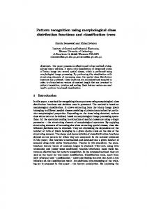
Fig. 1. The max-tree structure. Left: a 1-D signal; center: peak components Phk of the signal; right: its corresponding max-tree.

kernel) and fitted using bi-cubic splines. We use relations (4) to generate the knot sequence (t1 , t2 , . . . , tn ), and compute the curvature function κi (t) at each interpolated point, using spline derivatives. Finally, a curvature function κ0i (t) invariant with respect to rotations, translations and scaling transforms is computed using relation (3). C. From curvature to scale-space features In this section we present the morphological curvature scale spaces, and demonstrate causality of the extrema in the scale spaces. We also briefly describe the features extracted from the scale spaces, and study the behaviour of the scale-space representations under noise conditions. 1) Morphological curvature scale spaces: We begin with the definition of the hat-transform scale spaces [30], but unlike in [30], here we shall formulate the hat scale spaces in terms of the max-tree data structure [37]. The curvature scale spaces are particular 1-D versions of the hat-transform scale spaces, when the underlying 1-D signal is the curvature function. Let E be an arbitrary nonempty set of vertices, and denote by P(E) the collection of subsets of E. Also, let G = (E, Γ) be an undirected graph, where Γ is a mapping from E to P(E) which associates to each point x ∈ E the set Γ(x) of points adjacent to x. It is common in signal processing to assume that E is a regular grid, i.e. E ⊆ Zn (n = 1, 2), and Γ corresponds to 2-adjacency when n = 1, or to 4-adjacency or 8-adjacency when n = 2. In what follows we assume E ⊆ Zn , n = 1, 2. A path π in a graph G = (E, Γ) from point x0 to point xn is a sequence (x0 , x1 , ..., xn ) of points of E such that (xi , xi+1 ) are adjacent for all i ∈ [0, n). Let X ⊆ E be a subset of E. A set X is connected when for each pair (x0 , xn ) of points in X there exists a path of points in X that joins x0 and xn . A connected component of X is a connected subset C(X) of X which is maximal. A flat zone Lh at level h of a grey-scale signal f is a connected component C(Xh (f )) of the level set Xh (f ) = {p ∈ E|f (p) = h}. A regional maximum Mh at level h is a flat zone which has only strictly lower neighbours. A peak component Ph at level h is a connected component of the threshold set Th (f ) = {p ∈ E|f (p) ≥ h}. A connected opening Γx (X) extracts the connected component of X to which x belongs, if x ∈ X, and equals ∅ otherwise. Given a set A (the mask), the geodesic distance dA (p, q) between two pixels p and q is the length of the shortest path joining p and q which is included in A. The geodesic distance between a point p ∈ A and a set D ⊆ A is defined as dA (p, D) = mind∈D dA (p, d). A max-tree is a rooted tree, in which each of the nodes Chk at grey-level h corresponds to a peak component Phk . However,

IEEE TRANSACTIONS ON IMAGE PROCESSING, 2005, IN PRESS.

4

0 C 06 1 C 05

0 C 16

max(3,4) C 04

0 C 04

0 C 02

2 C 03

2 C 03

0 C 03

max(9,2) C 01

2 C 01

2 C 01

0 C 01

1 C 00

1 C 00

1 C 00

1 C 00

Fig. 2. Pruning a max-tree with the criterion Q(Phk ) using the max filtering rule. First row: Max-trees at iterations s = 0, 1, 2, 3; attributes A(Phk ) are shown in the left-hand side of each node Chk (the nodes for which the criterion T holds are marked; in every root path, Q holds for all nodes below a node for which T holds); second row: reconstructed signals fs .

Chk contains only those pixels in Phk which have grey level h. In other words, it is the union of all flat zones Ljh ⊆ Phk . An example of a 1-D signal, its peak components and its max-tree are shown in Fig. 1. Inspired by the work of Leymarie and Levine [28], we wish to split the curvature profile at points where the width of a feature suddenly changes. This can be formalized in terms of maximal distances of pixels of a max-tree node from its nearest child pixel. If this distance is larger than some threshold λ we consider this an abrupt change. Let f be a grey-scale image with an associated max-tree as in Fig. 1. Let Phk be a peak component at level h which has Nc peak components Phi + ⊆ Phk at level h+ , which is the smallest grey level larger than h, with i from some index set Ihk . The associated max-tree nodes are of course Chk and Chi + , respectively. Consider the attribute A(Phk ) defined as    max max (d(x, P i + )) h A(Phk ) = i∈Ihk x∈Phk  0

if Nc > 0

(5)

otherwise,

where d(x, Phi + ) denotes a distance measure from a pixel x to set Phi + . This distance might be the Euclidean or geodesic distance within Phk from x to the nearest member of Phi + . The filter criterion T which preserves nodes in the path from leaf to root where abrupt changes take place is T (Phk ) = (A(Phk ) > λ).

(6)

It is easy to see that this criterion is not increasing, so any max-tree filter γλT using it is an attribute thinning rather than an opening. The max filter rule for attribute thinnings proposed by Breen and Jones [19] will now allow us to remove branches of the max-tree at those points where the width suddenly changes. The max rule works by descending from each leaf of the max-tree, removing nodes until a node is found for which the criterion T is true. Any node between this node and the root is unaffected. A problem with the formulation of this filtering rule is that it is cast in terms of an algorithm. More formally, we can define a new criterion Q which takes

the max-rule into account Q(Phk ) =(A(Phk ) > λ) ∨ (∃x ∈ Phk , ∃h0 > h : A(Γx (Th0 (f ))) > λ).

(7)

Note that Γx (Th0 (f )) extracts a peak component Phi 0 ⊆ Phk . In other words, peak component Phk is preserved if it meets criterion T or if any peak component Phi 0 ⊆ Phk with h0 > h meets T . An example of filtering a max tree, using criterium Q according to the max rule is given in Fig. 2. Attribute thinning γλQ can now be defined as γλQ (f )(x) = max{h : Q(Γx (Th (f )))}.

(8)

Unlike most attribute thinnings, γλQ is not idempotent. It can be seen from (5) that all regional maxima will be removed for any positive λ, because A is zero for these peak components. However, any component for which Q is true in image f will have at least one nested peak component at h+ . Let Phk be such a component. There are two situations: (i) Q(Phi + ) is false for all i ∈ Ihk , or (ii) Q(Phi + ) is true for at least one i ∈ Ihk . In the first case, node Phk in the filtered image γλQ (f ) will be a regional maximum, and therefore be removed by a second application of γλQ . In the second case, it can easily be verified that there must exist a Phj0 ⊆ Phk , h0 > h, for which Q is true and for which the first case holds, because all regional maxima have A(Pji ) = 0. Therefore, unless there are no nodes in the max-tree of f for which Q is true, γλQ (γλQ (f )) 6= γλQ (f ). Then, letting d in (5) be the geodesic distance within Phk (i.e. d(x, Phi + ) = dPhk (x, Phi + )), and setting λ = 1 in (7), the top-hat scale space [30] of a grey-scale image f is given by the sequence (τ0 , τ1 , . . . , τS ) defined by the iteration fs+1 = γλQ (fs ) τs = fs − fs+1 ,

(9)

with f0 = f and s ≥ 0. Eq. (9) is iterated until fS = fmin for all pixels, where fmin is the minimum value of f . Using the grey-scale inversion f ↔ −f , a bottom-hat scale space can be formulated. Note that this formulation differs from that in [30]; however, it can be shown to be equivalent.

IEEE TRANSACTIONS ON IMAGE PROCESSING, 2005, IN PRESS.

f

0

f ,τ s

s

5

f0

0

fs, τs

1

1 2

Iteration (s)

2

Iteration (s)

0

3 4

3 4

5

5

6

6 7

7

0

50

100

Position along contour

150

0

50

100

Position along contour

150

Fig. 3. Building curvature spaces. Top: a binary image representing a complex object; left: curvature function (i.e. f0 ), residuals τs (in bold) and signals fs , s = 1, . . . , 7 represented in the top-hat scale space; right: curvature function, residuals τs and signals fs , s = 1, . . . , 7 represented in the bottom-hat scale space.

The curvature scale spaces are obtained by iterating relations (9) on the curvature function (i.e. f = κ0 ) and on its grey-scale inversion κ0 ↔ −κ0 . An example is shown in Fig. 3. Then, each extracted residual (i.e. peak of the curvature, represented in the top-hat scale space, and valley represented in the bottom-hat scale space) is described by its extremal curvature, mean curvature, extent and location. The scale spaces can be visualized by “reconstructing” the original signal in the following manner. We start with a constant signal f = 0. Then, we stack the boxes corresponding to the nested features (peaks) on top of one another, i.e. we accumulate their maximum (or average) values in f , at appropriate positions (given by the extents of the peaks) along the x axis; this has been done in Fig. 4. The current method is sensitive to differences in the relative locations of the curvature features. This means that, for example, an elongated rectangle and a square are distinguishable, because the widths of the major valleys in the curvature correspond to the distances between major peaks, so it is possible to discriminate between these. 2) Causality and monotonicity of the extrema in the hattransform scale spaces: An important characteristic of scalespace theory, in contrast to other multi-scale approaches, is the property that a signal feature present at some scale must be present all the way through scale-space to zero-scale (i.e. original signal) [18]. This is often called the causality principle and ensures that no new spurious features are created due to the filter. The stronger property of monotonicity requires that the number of features must decrease with increasing scale. There are several morphological scale-space representations which have been shown to obey the causality principle. Jackway and Deriche [18] proved that their dilation-erosion scale spaces have monotonic properties in two and higher dimensions, and do not cause features to be shifted by the smoothing. Extensive analysis of scale-space properties satisfied by n-dimensional sieves is given in [38]. It can be shown that the top-hat scale spaces (9) constitute a

special case of levelings [27], [39], a general nonlinear scalespace representation which satisfies the causality principle. However, since no complete proof was given in [27], [39], we will briefly analyze the behaviour of the extrema in the hat-transform scale space and prove that our scale-space representations fulfill these principles. Let Ps be the set of all peak components, and Ms the set of all regional maxima of fs , as defined in (9). Furthermore the set Rs is defined as Rs = {Phk ∈ Ps | ¬Q(Phk )}.

(10)

Obviously Ms ⊆ Rs , and Ps+1 = Ps \Rs . Finally, we define a set Qs as Qs = {Phk ∈ Ps \ Rs |∀i ∈ Ihk : Phi + ∈ Rs }.

(11)

In other words, Qs is the set of peak components Phk for which Q holds, but which have no Phi + ⊆ Phk for which Q holds. It can be seen that Qs = Ms+1 .

(12)

Each feature extracted from fs by γ1Q consists of precisely one member of Ms , and possibly a set of members of Rs \ Ms . For example, in the leftmost max-tree in Fig. 2 the maximum associated with C60 also contains non-maximum node C50 . Unless Ps \ Rs = ∅, a feature associated with regional maximum M ∈ Ms is associated with exactly one component Phk ∈ Ps \ Rs , which is the peak component at the highest grey level for which M ⊂ Phk and Q(Phk ) holds. Multiple maxima may be associated with any Phk , and Phk need not be a member of Qs . In Fig. 2, C40 is associated with two maxima: C60 and C61 . Furthermore, the peak component P10 represented by C10 in Fig. 2 is associated with maximum C20 , but P10 6∈ Q0 . Should Phk 6∈ Qs then there exists a component at a coarser scale than s which is nested within it. For these reasons, #(Qs ) = #(Ms+1 ) ≤ #(Ms ), with # denoting cardinality. Furthermore, if Ps 6= ∅ there must be at least one

IEEE TRANSACTIONS ON IMAGE PROCESSING, 2005, IN PRESS.

6

3

curvature reconstruction

1

Curvature

2

1

Curvature

noisy original

2

3

0

0

−1

−1

−2

−2

−3

−3

−4 0

50

100

150

Position along contour −4 0

50

100

150

Position along contour

3

noisy original

2 1 0

Curvature

Fig. 4. Left: original contour and sample points; right: curvature function (solid) superimposed on the reconstructed signal (bold) using top-hat scalespace information. Top and bottom scale spaces represented as curves, showing scale-space features as blocks of the correct width and maximum height.

−1 −2 −3

regional maximum, so #(Ps+1 ) < #(Ps ). If #(Ps ) > 1 we have #(Ms ) ≤ #(Ps − 1). This means that because the total number of peak components decreases strictly, the number of maxima must decrease for sufficiently large s, proving monotonicity. Furthermore any new maximum M ∈ Ms+1 of fs+1 is identical to a peak component P ∈ Qs of fs . Therefore, no new maxima are introduced, the number of maxima decreases, and there is an explicit nesting relationship between features at small and large scales in the scale space. Thus, the localization of the contours is preserved, and the causality principle is verified: coarser scales can only be caused by what happened at finer scales. Hence, the reduction of connected components for descending grey levels, by filtering the initial signal according to relations (9) ensures causality. This means that the location and shape of regional maxima and flat zones are preserved all the way through scale-space to zero-scale. By duality, a similar result can be formulated, regarding local minima in the bottom-hat scale space. 3) Coping with noise: We carried out an experiment to test the stability of the curvature scale spaces under noise conditions. Fig. 4 shows the initial contour, its curvature function, and the reconstructed curvature using information extracted from the top scale space (maximum heights). The computations were made using n = 150 sampled points (marked with ’x’ in the contour graph), and Gaussian smoothing of the sampled contour with σ = 3.0. Fig. 5 shows the same contour affected by significant amounts of uniform, random noise, added to it. The noisy contours were obtained by randomly translating the coordinates of each point in the intervals [−5; 5], and [−20; 20], respectively. As expected, the scale-space signals show differences in detail, cf. Fig. 5. However, remarkable similarities of the structures present in these graphs can be observed. The same behaviour is exhibited by the features extracted from the bottom-hat scale spaces (results not shown). This experiment shows that the curvature scale spaces are reliable and stable even when large amounts of noise corrupt the shape of the original curve. III. S CALE - SPACE DESCRIPTORS This section is devoted to the extraction of pattern vectors, based on the information stored in the scale spaces, and to the

−4 −5 0

50

100

150

Position along contour

Fig. 5. Left: contours affected by noise; right: reconstructed noisy curvature signals (bold) superimposed on the reconstruction of the original curvature (solid).

computation of a dissimilarity measure between two shapes, useful for shape matching. A. Extraction of pattern vectors In principle, knowledge of the curvature function is sufficient to determine a planar curve, up to a rigid transform. However, if a curve underwent non-rigid transforms and/or is affected by a large degree of noise, its curvature function would be affected accordingly. Although the very purpose of a scale-space representation is to gain robustness with respect to such factors, special care must be taken to address these problems. Since for regularization purposes, the input curves are smoothed with Gaussian kernels, selecting a suitable width σ for each curve is by no means trivial. To tackle this problem, a simple yet not very efficient solution is to smooth each curve successively by Gaussian kernels of increasing widths (i.e. σ1 < σ2 < · · · < σI ), and to build hat scale spaces at each iteration i = 1, 2, . . . , I. The final pattern vector is then constructed by concatenating the pattern vectors obtained at each iteration, from top and bottom scale spaces. Since the curvature function becomes smoother when the width of the Gaussian kernel increases, decreasing lengths of the pattern vectors extracted from the scale spaces are used. Let Nt (σi ) be the length of the pattern vector extracted at scale σi from the top scale space, and Nb (σi ) be the length of the pattern vector extracted from the bottom scale space. In order to further shorten the final pattern vector, we choose Nt and Nb such that Nt (σi ) ≥ Nb (σi ), i = 1, 2, . . . , I. Since curvature is a local attribute, additional global shape parameters are also computed at each iteration; we included two global curvature-related descriptors and two global shape descriptors. The first global curvature descriptor is the bending energy, defined as the sum of the squared curvatures along the contour. The second global curvature descriptor is defined as the number of scale space entries from both top and bottom

IEEE TRANSACTIONS ON IMAGE PROCESSING, 2005, IN PRESS.

7

scale spaces having average curvatures above a threshold tκ . This descriptor is similar to the curvature scalar descriptor, which is defined as the number of contour points where the boundary changes significantly, divided by the total length of the contour. The two global shape descriptors are eccentricity and elongation [40]. Note that similar global descriptors were also used in [9], [41] and in the MPEG-7 standard [42] to supplement the Curvature Scale Space (CSS) descriptors. Finally, the pattern vector extracted at iteration i, i = 1, 2, . . . , I is given by Vi = (ht,i,1 , ht,i,2 , . . . , ht,i,Nt (σi ) , hb,i,1 , hb,i,2 , . . . , hb,i,Nb (σi ) , p ecci , elgi , bei , csdi ),

(13)

where ecci , elgi , bei , csdi , are eccentricity, elongation, bending energy, and curvature scalar descriptor, respectively. The values ht,i,j , j = 1, . . . , Nt (σi ), represent the Nt (σi ) features with the largest maximum curvature extracted from the top scale space, at iteration i. Similarly, hb,i,j , j = 1, . . . , Nb (σi ), represent the Nb (σi ) features with the largest maximum curvature extracted from the bottom scale space, at iteration i. B. A measure of dissimilarity between shapes Let V be the final pattern vector representing the reference shape S, and V 0 be the final pattern vector corresponding to a test shape S 0 , obtained by concatenating the corresponding vectors Vi and Vj0 , i, j = 1, 2, . . . , I, as defined in (13); here s is the maximum scale index, as defined in subsection III-A. As is common in content-based retrieval literature, we define a measure of dissimilarity dSS 0 between shapes S and S 0 as the following weighted L1 distance   Nb Nt X X htj − h0tj + dSS 0 = w1  |hbk − h0bk | j=1

+ w2 + w3

s X

k=1

(|eccl − ecc0l | + |elgl − elgl0 |)

l=1 s X

(|bem − be0m | + |csdm − csd0m |) , (14)

m=1

Ps

Ps where Nt = i=1 Nt (σi ), Nb = i=1 Nb (σi ), and w1 , w2 , w3 are weights. The “prime” symbol indicates features corresponding to the test shape S 0 . IV. C ASE STUDIES To test the reliability of the proposed method for shapebased object recognition, we used three data sets, and for each of them we performed two types of recognition experiments: shape retrieval and shape identification. A content-based (or query by example) retrieval system contains a database of objects (e.g. images, shapes), and responds to a query object presented by the user with ranked similar objects. Usually these systems do not use a training stage and compute similarity between objects based on some distance measure. Contrary to content-based retrieval, in supervised shape identification a

Fig. 6.

Examples of contours extracted from the diatoms image set.

classification function is learned from, or fitted to, training data, and then the classifier is tested on unseen (test) data. For shape retrieval, the performance was measured using the so-called “bulls-eye test”, in which each shape contour is used as query and one counts the number of correct hits in the top 2 × K matches, where K is the number of prototypes per class. In our shape identification experiments we have used the C4.5 algorithm [43] for constructing decision trees, with bagging [44] as a method of improving the accuracy of the classifier. The performance was evaluated using the holdout [45] method. We compare the results obtained using our method with those obtained using Fourier descriptors (FD) [46], wavelet descriptors (WD) [14], and the CSS descriptors developed for the MPEG-7 standard (CSSD) [42]. In cases for which there are published results, other than those obtained with the above methods, we will also refer to them.

A. Pre-processing and settings of parameters For each technique, parameter values have to be determined that would give the best results for each data set. This involves an iterative process of initially guessing suitable parameter values, evaluating the results, and then refining the values. Since this is a time-consuming procedure, two points should be made: (i) the values used are not the result of an exhaustive search of the parameter space, because such a search would be impractical, requiring a very long time, and (ii) the parameter values were adjusted in an attempt to give best average performance, across all data sets. Although the values may not be optimal (as a consequence of the first observation), they produced the best classification performances in our experiments. The parameters of the morphological scale spaces were set as follows. Each input curve is sampled at an equal number of points, such that the resulting curve has n = 150 points. This curve is regularized by smoothing with Gaussian kernels of increasing width. We selected I = 4 values for the smoothing parameter σi : 3.0, 6.0, 10.0, 16.0, in an attempt to cover a large interval of smoothing degrees. The numbers of features extracted from both the top scale space and the bottom hat scale space were set to Nt (σi ) : 10, 10, 5, 5, and Nb (σi ) : 5, 5, 5, 5, respectively. Finally, the weights were set to w1 = 2.0, w2 = 0.5 and w3 = 3.0, and the threshold parameter was tk = 0.1. The parameters of the other methods were set according to [41], [42] for the CSS method, [14] for the WD, and [47] for the FD.

IEEE TRANSACTIONS ON IMAGE PROCESSING, 2005, IN PRESS.

TABLE I I DENTIFICATION PERFORMANCES FOR THE DIATOMS DATA SET (D IATOMS ), MPEG-7 SILHOUETTE DATABASE (MPEG-7) AND COIL-20 (COIL) DATABASE , USING THE C4.5 DECISION TREE CLASSIFIER WITH BAGGING . Data set

Descriptors

x ¯

σ

min

max

performance (%)

Diatoms

MCSSD CSSD FD WD

17.9 45.8 37.6 38.7

1.3 2.4 1.8 2.6

11 30 31 28

26 58 43 47

91.3 ± 5.0 75.4 ± 9.3 79.6 ± 7.0 79.0 ± 10.1

MPEG-7

MCSSD CSSD FD WD

31.5 76.4 114.9 98.6

1.6 1.4 1.6 1.8

22 51 108 83

41 91 122 115

91.9 ± 11.2 85.2 ± 9.8 67.2 ± 11.2 71.8 ± 12.6

COIL

MCSSD CSSD FD WD

3.4 10.9 16.6 12.3

0.5 0.4 0.8 0.9

1 8 10 7

8 15 22 18

98.0 ± 3.6 89.1 ± 2.8 83.4 ± 5.7 87.7 ± 6.4

B. Recognition of diatoms In the first experiment we measured identification and shape retrieval results on a large set of diatom images, which consists of 37 different taxa, comprising a total of 781 images. Each class (taxon) has at least 20 representatives. Diatoms are microscopic, single-celled algae, which show highly ornate silica shells or frustules. Some examples of diatom images are shown in Fig. 6. Each image represents a single shell of a diatom, and each diatom image is accompanied by the outline of its view (see Fig. 6). For additional details on diatoms, segmentation of diatom images, or other identification results than those presented here, we refer to [47], which contains the results of the Automatic Diatom Identification and Classification (ADIAC) project, aimed at automating the process of diatom identification by digital image analysis. With the experimental setup given in section IV-A and the identification technique briefly described at the beginning of section IV, the identification performances obtained by all methods for each data set are given in Table I. Similarly, retrieval performances obtained using the so-called “bullseye test” are given in Table II. Table I shows identification performances using the C4.5 decision tree classifier with bagging. The column ‘¯ x’ contains the average number of errors; the column ‘σ’ contains the standard deviation of the number of errors; the columns ‘min’ and ‘max’ contain the minimum and maximum number of errors, respectively; the column ‘performance’ contains the percentage (average with standard deviation) of samples identified correctly. In both tables, MCSSD stands for the morphological curvature scale space descriptor from section III-A, CSSD represents the curvature scale space descriptor, Fourier descriptors are denoted by FD, and the wavelet descriptors are denoted by WD. The performances obtained using MCSSD were at least 8 % larger than the others, while the identification performance for this data set is the best result obtained during the ADIAC

8

project [47]. Fourier and wavelet descriptors performed well, resulting in identification performances close to 80 %, and retrieval performances of almost 75 %. The poor performances obtained using the CSSD (based on inflection points) can be explained by the fact that most diatoms in this data set exhibit convex shapes and there are no inflection points on the contour of a convex object. Since the MCSS method extracts information about both convexities and concavities, our method is not upset by convex shapes. TABLE II S HAPE RETRIEVAL PERFORMANCES (%) FOR THE DIATOMS DATA SET (D IATOMS ), MPEG-7 SILHOUETTE DATABASE (MPEG-7) AND COIL-20 (COIL) DATABASE . Data set Diatoms MPEG-7 COIL

MCSSD 82.2 78.8 81.5

CSSD 66.0 73.4 71.4

FD 73.7 55.2 62.7

WD 74.2 58.5 64.3

C. Recognition using silhouettes. The MPEG-7 database Our next experiment was performed using the MPEG-7 shape silhouette data set, a database of 1400 objects used in the MPEG-7 Core Experiment CE-Shape-1 part B [48]. This database consists of 70 shape categories, with 20 objects per category. Using the same setup as in the first experiment, identification performances for this data set are shown in Table I, and retrieval performances are given in Table II. For this data set both methods based on curvature information performed much better than Fourier and wavelet descriptors. However, the MCSS method outperformed the CSS technique, yielding performances which are 5 % larger than those of the latter. Other published retrieval results for this data set, using the same methodology, do exist and range from 75.44 % to 78.38 % [41], [48–51]. A possible reason for achieving improved results is that our descriptor is invariant with respect to reflections, whereas shape contexts [51] and CSS descriptors [41] are not. This reflection invariance also holds for the method in [49], which has a performance of 78.38 %, but this method requires substantially more computation time than ours. Also, as shown in [48] there are cases in which shapes perceived as conceptually different have the same positions of the maxima of the CSS image, and hence the CSS method fails. D. 3-D object recognition based on 2-D views This experiment involved recognition of objects based on their 2-D appearances. We used the COIL-20 database [52]. Each of the 20 objects from this database is represented by 72 2-D views, corresponding to successive rotations of the object over an angle of 5◦ . Closed, outside contours were extracted using the Canny edge detector, followed by a contour-tracing algorithm [40]. Otherwise, we have used the same experimental setup as with the other experiments. For this data set, the number of prototypes can be reduced because some of the views of the objects have approximately

IEEE TRANSACTIONS ON IMAGE PROCESSING, 2005, IN PRESS.

the same appearance. Belongie et al. [51] report 2.4 % error rate using only four 2-D views for each object (i.e. 80 prototypes). They used a modified k-means clustering algorithm for adaptively selecting (and therefore reducing) prototypes, and a nearest-neighbour classifier. Instead of using more advanced clustering algorithms in order to further reduce the number of prototypes, we use the same experimental setup as in our previous experiments, and report the identification and retrieval performances shown in Tables I and II, respectively. Once again the performances obtained using MCSSD were at least 8 % larger then the others. For this data set, the CSS method outperformed the Fourier and wavelet methods.

V. C ONCLUSIONS We have proposed a multi-scale method for object recognition, based on contour information. The method is based on two morphological scale-space representations, the hattransform scale spaces, which showed successful applicability for shape-based recognition. These representations of the curvature signal result in a novel representation, the morphological curvature scale spaces. We demonstrated causality of the extrema in the scale spaces, an essential characteristic to any scale-space formulation. Besides this theoretical result, we have shown the relevance of these representations to object recognition and illustrated their usage for identification and shape retrieval. We evaluated the performance of the method in three recognition experiments: recognition of diatoms based on natural images of diatom shells, recognition using silhouettes from the MPEG-7 database, and 3-D object recognition based on 2-D views. Our method outperforms all shape comparison methods previously reported in the literature, in both identification and retrieval performances. The shape descriptor uses only maximum heights of the extrema of the curvature function and some global shape descriptors, and no information regarding the positions of the extrema along the contour. The advantage of this approach is that matching two shapes means simply computing a distance between the two descriptors, without any alignment (i.e. shifting) of the maxima as is required in the CSS method. Also, the method can be used for scale-invariant shape analysis, e.g. when a non-uniformly scaled square and a rectangle are assigned to the same class. However, if this is not desired, the descriptor can be augmented with the relative sizes of the extracted features to discriminate between such cases. The shape descriptor incorporates both convexities and concavities of shapes, and hence it is possible to discriminate between convex shapes. Furthermore, the method is robust to local shape deformations and copes well with large amounts of noise. Finally, the method is fast, and the computational complexity of constructing the scale spaces is linear in the number of points of the input contour. For example, the CPU time spent to compute and collect the shape descriptors for all 1400 contours of the MPEG-7 dataset is under two minutes on a Pentium III machine at 670 MHz.

9

R EFERENCES [1] A. P. Witkin, “Scale-space filtering,” in Proc. Int. Joint Conf. Artificial Intell., Palo Alto, CA, August 1983, pp. 1019–1022. [2] C. Fermuller and W. Kropatsch, “Multi-resolution shape description by corners,” in CVPR92, 1992, pp. 271–276. [3] E. Saund, “Adding scale to the primal sketch,” in CVPR89, 1989, pp. 70–78. [4] D. G. Lowe, Perceptual organization and visual recognition. Boston: Kluwer Academic Publishers, 1985. [5] R. Bajcsy and S. Kovacic, “Multiresolution elastic matching,” CVGIP, vol. 46, pp. 1–21, 1989. [6] F. Attneave, “Some informational aspects of visual perception,” Psychol. Rev., vol. 61, pp. 183–193, 1954. [7] J. R. Pomerantz, L. C. Sager, and R. J. Stoever, “Perception of wholes and their component parts: some configural superiority effects,” J. Exp. Psychol., vol. 3, pp. 422–435, 1977. [8] T. Pavlidis, “Algorithms for shape analysis of contours and waveforms,” IEEE Trans. Pattern Anal. Machine Intell., vol. 2, pp. 301–312, 1980. [9] F. Mokhtarian and A. K. Mackworth, “Scale-based description and recognition of planar curves and two-dimensional shapes,” IEEE Trans. Pattern Anal. Machine Intell., vol. 8, pp. 34–43, 1986. [10] ——, “A theory of multiscale, curvature-based shape representation for planar curves,” IEEE Trans. Pattern Anal. Machine Intell., vol. 14, pp. 789–805, 1992. [11] G. Dudek and J. K. Tsotsos, “Shape representation and recognition from multiscale curvature,” Comput. Vision Image Understand., vol. 68, pp. 170–189, 1997. [12] S. L. Yu-Ping Wang and K. T. Lee, “Multiscale curvature based shape representation using b-spline wavelets,” IEEE Trans. Image Processing, vol. 8, no. 11, pp. 1586–1592, 1999. [13] H. Asada and M. Brady, “The curvature primal sketch,” IEEE Trans. Pattern Anal. Machine Intell., vol. 8, pp. 2–14, 1986. [14] G. C.-H. Chuang and C.-C. J. Kuo, “Wavelet descriptor of planar curves: Theory and applications,” IEEE Trans. Image Processing, vol. 5, pp. 56– 70, 1996. [15] J. J. Koenderink, “The structure of images,” Biological Cybernetics, vol. 50, pp. 363–370, 1984. [16] A. L. Yuille and T. A. Poggio, “Scaling theorems for zero crossings,” IEEE Trans. Pattern Anal. Machine Intell., vol. 8, pp. 15–25, 1986. [17] L. M. Lifshitz and S. M. Pizer, “A multiresolution hierarchical approach to image segmentation based on intensity extrema,” IEEE Trans. Pattern Anal. Machine Intell., vol. 12, pp. 529–541, 1990. [18] P. T. Jackway and M. Deriche, “Scale-space properties of the multiscale morphological dilation-erosion,” IEEE Trans. Pattern Anal. Machine Intell., vol. 18, pp. 38–51, 1996. [19] E. J. Breen and R. Jones, “Attribute openings, thinnings and granulometries,” Computer Vision and Image Understanding, vol. 64, no. 3, pp. 377–389, 1996. [20] P. F. M. Nacken, “Chamfer metrics in mathematical morphology,” Journal of Mathematical Imaging and Vision, vol. 4, pp. 233–253, 1994. [21] J. A. Bangham, P. Chardaire, C. J. Pye, and P. D. Ling, “Multiscale nonlinear decomposition: the sieve decomposition theorem,” IEEE Trans. Pattern Anal. Machine Intell., vol. 18, pp. 529–538, 1996. [22] J. A. Bangham, P. D. Ling, and R. Harvey, “Scale-space from nonlinear filters,” IEEE Trans. Pattern Anal. Machine Intell., vol. 18, pp. 520–528, 1996. [23] B. B. Kimia and K. Siddiqi, “Geometric heat equation and nonlinear diffusion of shapes and images,” Comput. Vision Image Understand., vol. 64, pp. 305–322, 1996. [24] B. K. Jang and R. T. Chin, “Morphological scale space for 2d shape smoothing,” Comput. Vision Image Understand., vol. 70, pp. 121–141, 1998. [25] M. H. Chen and P. F. Yan, “A multiscale approach based on morphological filtering,” IEEE Trans. Pattern Anal. Machine Intell., vol. 11, pp. 694–700, 1989. [26] K.-R. Park and C.-N. Lee, “Scale-space using mathematical morphology,” IEEE Trans. Pattern Anal. Machine Intell., vol. 18, pp. 1121–1126, 1996. [27] F. Meyer and P. Maragos, “Morphological scale-space representation with levelings,” in Scale-Space’99, ser. Lecture Notes in Computer Science, M. Nielsen, P. Johansen, O. F. Olsen, and J. Weickert, Eds. Springer-Verlag Berlin Heidelberg, 1999, vol. 1682, pp. 187–198. [28] F. Leymarie and M. D. Levine, “Shape features using curvature morphology,” in Proceedings SPIE, ser. Visual Communications and Image Processing IV, vol. 1199, 1989, pp. 390–401.

IEEE TRANSACTIONS ON IMAGE PROCESSING, 2005, IN PRESS.

[29] P. Salembier and J. Serra, “Flat zones filtering, connected operators, and filters by reconstruction,” IEEE Trans. Image Processing, vol. 4, pp. 1153–1160, 1995. [30] A. C. Jalba, M. H. F. Wilkinson, and J. B. T. M. Roerdink, “Morphological hat-transform scale spaces and their use in pattern classification,” Pattern Recognition, vol. 37, pp. 901–915, 2004. [31] G. Farin, Curves and Surfaces for Computer-Aided Geometric Design: A Practical Guide. San Diego: Academic Press, 1997. [32] L. Davis, “Understanding shape : angles and sides,” IEEE Trans. Comput., vol. 26, pp. 236–242, 1977. [33] G. Medioni and Y. Yasumoto, “Corner detection and curve representation using cubic b-splines,” CVGIP, vol. 39, pp. 267–278, 1987. [34] C. de Boor, A practical guide to splines. New York: Springer-Verlag, 1978. [35] P. J. van Otterloo, A Contour-Oriented Approach to Shape Analysis. Hemel Hampstead: Prentice Hall, 1992. [36] E. T. Y. Lee, “Choosing nodes in parametric curve interpolation,” Computer-Aided Design, vol. 21, pp. 363–370, 1989. [37] P. Salembier, A. Oliveras, and L. Garrido, “Anti-extensive connected operators for image and sequence processing,” IEEE Trans. Image Processing, vol. 7, pp. 555–570, 1998. [38] J. A. Bangham, R. Harvey, P. D. Ling, and R. V. Aldridge, “Morphological scale-space preserving transforms in many dimensions,” Journal of Electronic Imaging, vol. 5, pp. 283–299, 1996. [39] F. Meyer, “From connected operators to levelings,” in Mathematical Morphology and its Applications to Image and Signal Processing, H. Heijmans and J. Roerdink, Eds. Kluwer, 1998, pp. 191–199. [40] A. K. Jain, Fundamentals of digital image processing. Prentice Hall, 1989. [41] F. Mokhtarian, S. Abbasi, and J. Kittler, “Efficient and robust retrieval by shape content through curvature scale space,” in Image DataBases and Multi-Media Search, A. W. M. Smeulders and R. Jain, Eds. World Scientific Publishing, 1997, pp. 51–58. [42] M. Bober, “MPEG-7 visual shape descriptors,” IEEE Trans. on Circ. Syst. Vid. Tech., vol. 11, pp. 716–719, 2001. [43] J. R. Quinlan, C4. 5: Programs for Machine Learning. Morgan Kaufmann Publishers, 1993. [44] L. Breiman, “Bagging predictors,” Machine Learning, vol. 24(2), pp. 123–140, 1996. [45] R. Kohavi, “A study of cross-validation and bootstrap for accuracy estimation and model selection,” in International Joint Conference on Artificial Intelligence, 1995, pp. 1137–1145. [46] C. T. Zahn and R. Z. Roskies, “Fourier descriptors for plane closed curves,” IEEE Trans. Comput., vol. 21, pp. 269–281, 1972. [47] H. du Buf and M. M. Bayer, Eds., Automatic Diatom Identification. Singapore: World Scientific Publishing, 2002. [48] L. J. Latecki, R. Lakimper, and U. Eckhardt, “Shape descriptors for nonrigid shapes with a single closed contour,” in Proc. IEEE CVPR, 2000, pp. 1424–1429. [49] C. Grigorescu and N. Petkov, “Distance sets for shape filters and shape recognition,” IEEE Trans. Image Processing, vol. 12, pp. 1274–1286, 2003. [50] T. B. Sebastian, P. N. Klein, and B. B. Kimia, “On aligning curves,” IEEE Trans. Pattern Anal. Machine Intell., vol. 25, no. 1, pp. 116–124, 2003. [51] S. Belongie, J. Malik, and J. Puzicha, “Shape matching and object recognition using shape contexts,” IEEE Trans. Pattern Anal. Machine Intell., vol. 24, no. 4, pp. 509–522, 2002. [52] H. Murase and S. Nayar, “Visual learning and recognition of 3-d objects from appearence,” Int. J. Comp. Vis., vol. 14, no. 1, pp. 5–24, 1995.

10

Andrei C. Jalba received his B.Sc. (1998) and M.Sc. (1999) in Applied Electronics and Information Engineering from “Politehnica” University of Bucharest, Romania. He recently obtained a Ph.D. degree at the Institute for Mathematics and Computing Science of the University of Groningen, where he now is a postdoctoral researcher. His research interests include computer graphics and vision, image processing, and parallel computing.

Michael Wilkinson obtained an M.Sc. in astronomy from the Kapteyn Laboratory, University of Groningen (RuG) in 1993, after which he worked on image analysis of intestinal bacteria at the Department of Medical Microbiology, RuG. This work formed the basis of his Ph.D. at the Institute of Mathematics and Computing Science (IWI), RuG, in 1995. He was appointed as researcher at the Centre for High Performance Computing (also RuG) working on simulating the intestinal microbial ecosystem on parallel computers. During that time he edited the book “Digital Image Analysis of Microbes” (John Wiley, UK, 1998) together with Frits Schut. After this he worked as a researcher at the IWI on image analysis of diatoms. He is currently assistant professor at the IWI.

Jos B. T. M. Roerdink received his M.Sc. (1979) in theoretical physics from the University of Nijmegen, the Netherlands. Following his Ph.D. (1983) from the University of Utrecht and a two-year position (1983-1985) as a Postdoctoral Fellow at the University of California, San Diego, both in the area of stochastic processes, he joined the Centre for Mathematics and Computer Science in Amsterdam. There he worked from 1986-1992 on image processing and tomographic reconstruction. He was appointed associate professor (1992) and full professor (2003), respectively, at the Institute for Mathematics and Computing Science of the University of Groningen, where he currently holds a chair in Scientific visualization and Computer Graphics. His current research interests include biomedical visualization, neuroimaging and bioinformatics.