Nov 9, 2015 - faced by data collectors and analysts, consider the famous study by ... meet the goal of sharing social network data, in the form of synthetic ...
arXiv:1511.02930v1 [stat.CO] 9 Nov 2015
Sharing Social Network Data: Differentially Private Estimation of Exponential-Family Random Graph Models Vishesh Karwa and Pavel N. Krivitsky and Aleksandra B. Slavkovi´ c Abstract: Motivated by a real-life problem of sharing social network data that contain sensitive personal information, we propose a novel approach to release and analyze synthetic graphs in order to protect privacy of individual relationships captured by the social network while maintaining the validity of statistical results. Two case studies demonstrate the application and usefulness of the proposed techniques in solving the challenging problem of maintaining privacy and supporting open access to network data to ensure reproducibility of existing studies and discovering new scientific insights that can be obtained by analyzing such data. We use a simple yet effective randomized response mechanism to generate synthetic networks under �-edge differential privacy. We combine ideas and methods from both the statistics and the computer sciences, by utilizing likelihood based inference for missing data and Markov chain Monte Carlo (MCMC) techniques to fit exponential-family random graph models (ERGMs) to the generated synthetic networks.
1. Introduction Networks are a natural way to summarize relationship information among entities (such as individuals or organizations)—they allow one to model not only the attributes of entities but also the relations between them. Such relational data have become a prominent source of scientific inquiry for researchers in economics, epidemiology, sociology and many other disciplines. However, network data very often contain sensitive relational information (e.g., sexual relationships, or email exchanges). While the social benefits of analyzing such data are significant, any privacy breach of the relational information can cause public shame and even economic harm to the privacy of individuals and organizations involved. With the increase in the quantity of data being collected and stored, such privacy risks are bound to increase. In contrast to these privacy issues is the need to allow open access to data to ensure reproducibility of existing studies and to discover new scientific insights that can be obtained by analyzing such data. As a typical example of the tension faced by data collectors and analysts, consider the famous study by Bearman, Moody and Stovel (2004), where researchers analyzed a rich dataset of social network of high school students to study their romantic relationships, and more broadly to understand the structure of human sexual networks. However, access 1
V. Karwa and A. Slavkovi´ c and P. Krivitsky/Sharing Social Network Data]
2
to such network data is typically limited due to obvious privacy concerns, and examples abound. In two case studies in this paper, we consider the above mentioned problem of limiting disclosure risk of relational information while allowing for statistical utility in the context of two network datasets—A teenage friendship and substance use network formed from the data collected in the Teenage Friends and Lifestyle Study (Michell and Amos, 1997; Pearson and Michell, 2000) for a cohort of students in a school in Scotland, and a network formed from the collaborative working relations between n = 36 partners in a New England law firm (Lazega, 2001). We consider varying privacy risks for relations (represented by dyads) that depend on the nature of node attributes. Limiting the disclosure risk while allowing for the data to remain useful has been the subject of many studies in statistics and data mining, and numerous techniques have been developed in the fields of statistical disclosure limitation (SDL) and privacy-preserving data mining, albeit with a limited focus on network data; for more on SDL methods which focus on statistical methodology to address this inherent trade-off, see for example, (Fienberg and Slavkovi´c, 2010; Hundepool et al., 2012). A drawback of these techniques is that in most cases they do not offer any formal privacy guarantees—whether or not a disclosure technique makes the data “safe” to release is left to the subjective decision of data curator and the risk is highly dependent on the assumed knowledge of what additional information the potential intruder may have. Due to this, “naive” privacy-preserving methods such as anonymization (e.g., by removing the basic identifiers such as name, social security number, etc.), have been shown to fail and can lead to disclosure of individual relationships or characteristics associated with the released network (for more specific examples, see Narayanan and Shmatikov (2009) and Backstrom, Dwork and Kleinberg (2007)). To overcome such issues, one needs a principled and formal way to reason about how to measure and limit the privacy risks of data release mechanisms over multiple data releases. We use the framework of differential privacy (DP) (Dwork et al., 2006a) to meet the goal of sharing social network data, in the form of synthetic networks, while protecting the privacy of individual relationships. DP has emerged, from the theoretical computer science community, as a principled way to provably limit a worst case disclosure risk across multiple data releases in presence of any arbitrary external information1 Any data release mechanism (method) that satisfies differential privacy comes with strong worst case privacy guarantees. A significant amount work on DP has been done in the theoretical computer science, and some in statistics. However, a common criticism of DP is that it may be too strong of a guarantee for statistical applications and more importantly, the primary focus of DP-based techniques is on releasing summary statistics of the data, as opposed to performing statistical inference (e.g. parameter inference). To address the latter issue, we adopt ideas and techniques from missing 1 We want to point out that Differential privacy (DP) is not the first framework to quantify disclosure risk, which has been a subject of research in the SDL area. However, the DP risk measure is the first one that composes, i.e., the degradation of disclosure risk can be controlled over multiple data releases. Hence it allows for a modular design of data release mechanisms.
V. Karwa and A. Slavkovi´ c and P. Krivitsky/Sharing Social Network Data]
3
data methods to ensure that one can perform valid statistical inference on differentially private synthetic networks. The work in this paper, builds on the initial ideas and examples presented in Karwa, Slavkovi´c and Krivitsky (2014), which was the first to develop techniques for actually fitting and estimating a wide class of Exponential-Family Random Graph Models (ERGMs) in a differentially private manner. We focus on ERGMs since they have become the workhorse for analyzing social network data (Goodreau, Kitts and Morris, 2009; Robins et al., 2007; Goldenberg et al., 2010). Previous studies in privacy of network data have focused on releasing noisy summary statistics that correspond to sufficient statistics of ERGMs. For example, Karwa et al. (2011) use the smooth sensitivity framework of Dwork et al. (2006a) to add noise and release subgraph counts such as number of ktriangles and k-stars, sufficient statistics for a wide class of ERGMs (Hunter, Goodreau and Handcock, 2008) and Hay et al. (2009) propose an algorithm for releasing the degree partition of a graph using the co-called Laplace mechanism along with post-processing techniques to reduces the L2 error between the true and the released degree distribution. These studies, however, fall short of demonstrating how to perform valid statistical inference using the noisy statistics, which is a non-trivial task, as discussed and demonstrated in the context of a class of ERGMs known as β model by Karwa and Slavkovi´c (2015); Karwa and Slavkovic (2012); for related issues of non-existence of maximum likelihood estimators (MLEs) for log-linear models of contingency tables, see Fienberg, Rinaldo and Yang (2010). Ignoring the noise addition process, which is often done in the case of private release of summary statistics or synthetic data, can lead to inconsistent and biased estimates – as already well established in the statistics literature, e.g., see Carroll et al. (2012). Motivated by the literature on the measurement error models, Karwa and Slavkovi´c (2015) take the noise addition process into consideration and construct a differentially private asymptotically normal and consistent estimator of the β model to achieve valid inference. But the main technique that relies on projecting the noisy sufficient statistics onto the lattice points of the marginal polytope corresponding to the β model does not scale well to more general ERGMs. To broaden the scope of private sharing of social network data, Karwa, Slavkovi´c and Krivitsky (2014) took a principled approach, rooted in likelihood theory, to perform inference from data released by privacy preserving mechanisms. The key idea is to release network data using a differentially private mechanism and estimate the parameters of ERGMs by taking into account the privacy mechanism. Thus, let X = x be the data that requires protection and let Pθ (X = x) be a model one is interested in fitting. Privacy preserving mechanisms can be modeled as Pγ (Y = y|X = x), i.e., the released data y is a sample from Pγ (Y = y|X = x) whose parameters γ of the privacy mechanism are publicly known. Most of the current work advocates on using Pθ (Y = y) for inference, ignoring the privacy mechanism. Declaring the original data x as missing, they develop methods that take Pthe privacy mechanism into account. They use the likelihood Pθ,γ (Y = y) = x Pγ (Y = y|X = x)Pθ (X = x) for in-
V. Karwa and A. Slavkovi´ c and P. Krivitsky/Sharing Social Network Data]
4
ference. This approach offers both the improved accuracy in estimation of θ and meaningful estimates of standard errors. In a related approach, Lu and Miklau (2014) propose to release the perturbed sufficient statistics of the model of interest, and describe a Bayesian exchange algorithm for recovering the parameters based on the perturbed statistics. In this paper, we improve on methods and results from Karwa, Slavkovi´c and Krivitsky (2014). We combine ideas and methods from both the statistics and the computer sciences, by utilizing likelihood based inference and Markov chain Monte Carlo (MCMC) techniques to fit ERGMs to produce synthetic networks in a differentially private manner, and thus simultaneously offer rigorous privacy guarantees and analytic validity. More specifically, in Section 2 we use the randomized response mechanism to release networks under �-edge differential privacy. The risk of privacy is measured by �, a parameter that controls the multiplicative odds of disclosure risk of any edge. The new algorithm allows for different levels of privacy risk for different types of dyads depending on the potential sensitivity of the connections, based on the nodal attributes. In Section 3, we present an improved MCMC algorithm for evaluating the utility in the framework of fitting ERGMs with private synthetic networks. In Section 4, two aforementioned case studies demonstrate the application and usefulness of the proposed techniques in solving the challenging problem of maintaining privacy and supporting open access to network data to ensure reproducibility of existing studies and discovering new scientific insights that can be obtained by analyzing such data. In Section 5 we discuss overall ramifications of sharing and some future directions. 2. Differential privacy for networks and Randomized response 2.1. Edge Differential Privacy We use the edge differential privacy (EDP) framework to measure the worst case risk of identifying any relationship when data is released in the form of a synthetic network. We focus on simple undirected networks for simplicity, but the results are straightforward to extend to directed networks. Simple networks are networks with no directed edges, and with no self loops and multiple edges. Let X be an undirected simple graph on n nodes with m edges. Let X denote the set of all simple graphs on n nodes. The distance between two graphs X and X 0 , is defined as the number of edges on which the graphs differ and is denoted by ∆(X, X 0 ). Each node can have a set of p attributes associated with it. These attributes can be collected in the form of a n × p matrix of covariates Z. We will assume that the matrix Z is known and public or has been released using an independent data release mechanism. Thus, we are interested in protecting the relationship information in the network X. Edge differential privacy is defined to measure the worst case disclosure risk of identifying any relationship (represented by edges) between entities (represented by nodes). To introduce the risk measure, note that any privacy preserving
V. Karwa and A. Slavkovi´ c and P. Krivitsky/Sharing Social Network Data]
5
mechanism can be modeled as a family of conditional probability distributions, denoted by Pγ (Y = y|X = x). Here x is the network that requires privacy protection and Y denotes the random synthetic network. Thus, the synthetic networks are samples from Pγ (Y = y|X = x). Let x and x0 be any two networks that differ by one edge. EDP bounds the worst case ratio of the likelihoods of Y conditional on x and x0 . More precisely, we say that the mechanism Pγ (Y = y|X = x) is � edge-differentially private iff max
x,x0 :∆(x,x0 )=1
log
Pγ (Y = y|X = x) ≤� Pγ (Y = y|X = x0 )
Edge differential privacy (EDP) requires that the distribution of data release mechanism on two neighboring networks (i.e., they differ by one edge) should be close to each other. The parameter � controls the amount of information leakage and measures the disclosure risk. Smaller values of � lead to lower information leakage and hence provide stronger privacy protection. One can show that even if an adversary knows all but one edge in the network, differential privacy ensures that the adversary cannot accurately test the existence of the unknown edge. Wasserman and Zhou (2010) formalize this property using the notion of a hypothesis test and show that there exist no hypothesis test that has any power to detect the presence (or absence) of any unknown edge, even if the adversary knows all the other edges. Another key property of differential privacy is that any function of the differentially private algorithm is also differentially private, without any loss in the disclosure risk, as measured by �, as the following lemma illustrates. Lemma 1 (Post-processing Dwork et al. (2006b); Nissim, Raskhodnikova and Smith (2007)). Let f be an output of an � differentially private algorithm applied to a graph X and g be any function whose domain is range of f . Then g(f (X)) is also � differentially private. Such strong guarantees make the framework of differential privacy very attractive to use for sharing data. However, the framework of Differential privacy is designed with an eye towards interactive data access mechanism and a focus on releasing summary statistics of the data, as opposed to sharing synthetic data for statistical inference. Indeed, most differentially private mechanisms are designed to release summary statistics of the data by adding noise to the output of a function f applied to a dataset, we call such data release mechanisms output perturbation mechanisms. A basic output perturbation mechanism for releasing any summary statistic f (x) called Laplace mechanism uses Laplace noise addition (e.g., see Dwork et al. (2006a)) to release differentially private noisy summary statistics. More specifically, the Laplace mechanism adds Laplace noise to f (x) proportional to its global sensitivity, which is the maximum change in f over neighboring networks. As an example, let f (x) ne the number of edges in the network. The global sensitivity of f (x) is 1, since adding or removing a single edge changes the edge count by 1. As a non-trivial example, let f (x) count the number of triangles. The global sensitivity in this case is O(n2 ) and hence
V. Karwa and A. Slavkovi´ c and P. Krivitsky/Sharing Social Network Data]
6
very large. One can also add noise proportional to the so called smooth version of local sensitivity, see Karwa et al. (2011). However, such output perturbation mechanisms that release noisy summary statistics are not suitable for releasing synthetic graphs for estimating a large class of ERGMs. This is because in order to use the Laplace Mechanism, we need to fix a set of models apriori and release the corresponding sufficient statistics. This limits the number of possible models one can fit. Moreover, the noisy summary statistics are not usable for estimating model parameters and performing statistical inference, see Fienberg, Rinaldo and Yang (2010), Karwa and Slavkovic (2012). A related issue is that estimating the sensitivity of many summary statistics is NP hard, see Karwa et al. (2011) for details. An alternative way is to perturb the network directly. We call such algorithms input perturbation algorithms. Randomized response is the simplest example of an input perturbation algorithm where random variables are perturbed by a known probability mechanism. Such designs have been extensively used and studied in the context of surveys when eliciting answers to sensitive questions, e.g., see the monograph by Chaudhuri (1987). It has also been used for statistical disclosure control when releasing data in the form of contingency tables, e.g., see Hout and Heijden (2002). We will use a randomized response mechanism to release dyads of a network, that is subgraphs of size 2, and generate a synthetic graph. 2.2. Randomized Response for networks Let X be a random graph with n nodes, represented by its adjacency matrix. The adjacency matrix is a binary n × n matrix with zeros on its diagonal, such that xij = 1 if there an edge from node i to node j, 0 if there is no edge, or non-edge between nodes i and j. Every node is labeled and there can be a set of variables associated with each node, that are assumed to be public. Considering the graph as a collection of labeled nodes and dyads that represent the ties between each nodes, we will apply randomized response to each dyad of the adjacency matrix of X. More specifically, for each dyad (i, j) let pij be the probability that the mechanism retains an edge if present, and qij be the probability that the mechanism retains a non-edge. Algorithm 1 shows how to release a random graph Y from X that is �-edge differentially private. Note that binary dyads. for an undirected graph, we need to release n(n−1) 2 Proposition 1. Let the privacy risk of each dyad i, j be � � qij 1 − pij 1 − qij pij �ij = log , , , 1 − pij qij pij 1 − qij Algorithm 1 is �-edge differentially private with � = maxij eij . Proposition 1 shows that Algorithm 1 is � differentially private The worst case privacy risk of Algorithm 1 as measured by � is determined by the most “revealing” dyad (i, j), i.e., any dyad (i∗ , j ∗ ) that achieves the maximum in
V. Karwa and A. Slavkovi´ c and P. Krivitsky/Sharing Social Network Data]
7
Algorithm 1 Dyadwise randomized response. 1: Let x = {xij } be the vector representation of the adjacency matrix of X 2: for each dyad xij do 3: if xij = 1 then ( 1 with probability pij 4: Let yij = 0 otherwise 5: else ( 1 with probability 1 − qij 6: Let yij = 0 otherwise 7: end if 8: Let Yi,j = {yij }. 9: end for 10: return Y
Proposition 1. This is because in the EDP framework, risk of any data release mechanism is measured by it’s worst case disclosure risk. For any dyad (i, j), if pij or qij is equal to 1 or 0 we get � = ∞, which in the EDP model represents infinite risk or no privacy. Hence to obtain finite privacy risks, no dyad can be left unperturbed—under EDP, every dyad has a positive probability of being perturbed. On the other hand if for all dyads, pij = qij = 0.5, then � = 0. This setting of parameters has 0 risk and provides the maximum possible privacy protection, but it also has 0 utility, as all the information in the original network is lost and there is no identifiability. We get a range of � from 0 to ∞ for intermediate values of pij and qij . We will assume that the parameters of Algorithm 1 are public, i.e., the matrix of values of pij and qij ’s are known, otherwise the parameters of any model to be estimated from the released network will not be identifiable. This does not increase the privacy risks as the privacy protection comes from the randomness inherent in the mechanism and not in the secrecy of the parameters of the mechanism. The worst case privacy risk is determined by the dyad that is most “revealing” or has the highest �ij in Proposition 1. On the other hand, if we deem the disclosure of one set of dyads to be more harming than other, we can define a different risk measure for groups of dyads by specifying a different value of � for different groups of dyads. In particular, consider partitioning the nodes into K groups of nodes, where the groups are labeled by k = 1, . . . , K. We can limit the privacy risk of dyads between nodes of Group k1 and Group k2 by specifying a K ×K matrix of � values. The (ki , kj ) entry of this matrix specifies the maximum tolerable privacy risk of dyads between nodes in group ki and ki . The worst case risk will still be determined by the maximum of all the �ki ,kj . However, in practice, it may be acceptable to increase the risk of some dyads while decreasing the risk of others, in order to obtain more utility. A very important point to note is that the choice of risk should depend only on publicly available information. For example, the choice of risk cannot depend on the existence of an edge in the network or the total number of edges between a group of nodes. In our framework, the risk choice can depend on the attributes of the nodes as this information is assumed to be public. As a concrete example that we further
V. Karwa and A. Slavkovi´ c and P. Krivitsky/Sharing Social Network Data]
8
illustrate in the case studies, one may deem that the re-identification of ties between nodes of same gender in a sexual network to be more devastating to the participants of the network when compared to ties between different gender. In such a case, we may assign a lower value of � (lower risk) for dyads between nodes of same sex, and a higher value of � for all other dyads. Note that the overall worst case risk is still determined by the largest �, but this setup allows one to take different risks into account. We use this strategy in the case studies in Section 4. Many different values of pij and qij amount to the same risk as measured by �ij for a single dyad. In particular, there are infinitely many values of pij and qij that give rise to the same �ij . The region of feasible values of pij and qij form a rhombus and are given in Lemma 2. Lemma 2. Let �ij be fixed, then the region of feasible values for pij and qij is given by a rhombus defined by LB(pij ) ≤ qij ≤ U B(pij ) with ( 1 − e�ij pij if 0 < pij < 1+e1�ij , LB(pij ) = −�ij e (1 − pij ) if 1+e1�ij < pij < 1 ( e�ij 1 − e−�ij pij if 0 < pij < 1+e � U B(p11 ) = . �ij e e�ij (1 − pij ) if 1+e �ij < pij < 1
A natural question to ask is given a fixed value of �ij , how can we choose the optimal values of pij and qij . The question of optimal values of pij and qij depends on how one measures utility and the risk. A simple criteria that we use is the following—for a given value of worst case risk, we want to ensure that the synthetic network is as close to the original network as possible, i.e. we want pij and qij to be as close to 1 as possible for a fixed value of � = maxij �ij . It is easy to see from Lemma 2 that for a fixed value of �ij , since the region of feasible values of pij and qij is a rhombus, the optimal occurs at one of the corners. This corner is when pij = qij . Thus, for each dyad (i, j), we choose πij e�ij pij = qij = πij = 1+e �ij . This gives us �ij = log 1−πij . Furthermore, if we want to limit the worst case risk by �, it is clear that it is optimal to choose each �ij = �. This is because �ij is an monotonic function of πij , and we want to maximize πij . Thus it is optimal to set �ij to its maximum possible value of �. A similar conclusion holds when considering privacy risks for groups of dyads. The above discussion shows that assuming that we want to limit the worst case risk for all dyads (or all dyads in a group) and maximize the probability of retaining the true state of a dyad, it is optimal to set pij = qij = π, where π is the probability of retaining a dyad in its original state. This is a special case of Algorithm 1, where we flip the state of each dyad with probability 1 − π. In this special case, the synthetic network has the following conditional distribution: Y Pπ (Y = y|X = x) = (1 − π)Iyij 6=xij (π)Iyij =xij , ij
where Iyij =xij takes value 1 if the same edge between i and j occurs in graphs x and y and zero otherwise. Note that as before, if π = 0.5, we cannot perform
V. Karwa and A. Slavkovi´ c and P. Krivitsky/Sharing Social Network Data]
9
any inference on a model for X as all information in the original data is lost. Moreover, if π < 0.5, the structure of graph “reverses”, i.e., edges become �nonedges and vice-versa. Hence to provide non-trivial utility, we set π ∈ 12 , 1 . In the next section we review exponential-family random graph models and present a method to estimate the parameters of any ERGM using the synthetic networks generated using Algorithm 1. 3. Likelihood based inference of ERGMs from randomized response Exponential-family random graph models (ERGMs) (Wasserman and Pattison, 1996, and others) express the probability of a network x ∈ X as an exponential family: exp{θ·g(x)} , x ∈ X, (1) Pθ (X = x) = c(θ, X ) with θ ∈ Θ ⊆ Rq a vector of parameters, g(x) a vector of sufficient statistics typically embodying the features of the social process that are of interest or are believed to be affecting the nextwork structure, and c(θ, X ) is the normalizing constant given by X c(θ, X ) = exp{θ·g(x)}. (2) x∈X
In absence of any privacy mechanism, x is a fully observed network from the model given by equation (1). One of the main challenges in finding the maximum likelihood estimate (MLE) of θ is that the normalizing constant c(θ, X ) given by (2) is intractable due to the sum over all possible graphs in X . A lot of work has been done in estimating the normalizing constant and maximizing the likelihood for estimating ERGMs. For example, Geyer and Thompson (1992) use a stochastic algorithm to compute the MLE for a large class of models that includes ERGMs (Hunter and Handcock, 2006). They approximate the normalizing constant using a Markov chain Monte Carlo (MCMC) algorithm, and compute the MLE by maximizing the stochastic approximation of the likelihood ˆ and let X1 , X2 , . . . , XM ratio. More precisely, let θ0 ∈ Θ be an initial guess for θ, ind ∼ Pθ0 (X = x), a random sample of M realizations from the model at θ0 , simulated using MCMC (Snijders, 2002; Handcock, 2003; Morris, Handcock and Hunter, 2008). Then, X exp{θ · g(x0 )} c(θ, X ) = c(θ0 , X ) c(θ0 , X ) 0 x ∈X
≈
M 1 X exp {(θ − θ0 )·g(Xi )}, M i=1
(3)
Maximizing this ratio with respect to θ to obtain the next guess θ1 , simulating ˆ from that, and repeating to convergence yields the MLE θ. The above algorithm used to approximate the likelihood can be extended to infer θ from a private sample y using a technique similar to that of Handcock et al. (2010) in the context of networks for which not all dyads are observed.
V. Karwa and A. Slavkovi´ c and P. Krivitsky/Sharing Social Network Data]
10
Recall that we wish to estimate θ using a private sample y obtained by drawing one realization from Pγ (Y = y|X = x). A naive approach is to ignore the privacy mechanism and estimate the parameters using the naive likelihood Pθ (X = y). The correct approach is to include the privacy mechanism in the model and use the full likelihood of Y . We can formulate this likelihood by treating the original data x as missing by design, and summing over all possible values of x that P could have, with the privacy mechamism, produced y: Ly,γ (θ) = P Pθ,γ (Y = y) = x∈X Pθ,γ (Y = y ∧ X = x) = x∈X Pγ (Y = y|X = x)Pθ (X = x). Thus, the maximum likelihood estimator of θ obtained from y X θˆMLE (y) = arg max Ly (θ) = arg max Pθ (X = x)Pγ (Y = y|X = x). (4) θ∈Θ
θ∈Θ
x∈X
In case of the randomized response mechanism of Algorithm 1, γ = π. Now, consider, as before, the likelihood ratio of θ with respect to some initial configuration θ0 : P exp{θ·g(x)} Pγ (Y = y|X = x) Ly,γ (θ) x∈X c(θ,X ) =P exp{θ ·g(x)} 0 Ly,γ (θ0 ) Pγ (Y = y|X = x) x∈X
c(θ0 ,X )
exp{θ0 ·g(x)}Pγ (Y = y|X = x) c(θ0 , X ) X exp{(θ − θ0 )·g(x)} P . = 0 0 c(θ, X ) 0 x ∈X exp{θ0 ·g(x )}Pγ (Y = y|X = x ) x∈X
In the above expression, the ratio of normalizing constants can be approximated as in (3), while the summation is a conditional expectation of exp{(θ − θ0 )·g(x)} with respect to an ERGM with parameter θ0 , given that y was observed. A Metropolis algorithm that samples symmetrically over X and accepts with probability � � � � exp{θ0 ·g(x? )}Pγ (Y = y|X = x? ) Pγ (Y = y|X = x? ) ? min 1, = min 1, exp[θ0 ·{g(x ) − g(x)}] , exp{θ0 ·g(x)}Pγ (Y = y|X = x) Pγ (Y = y|X = x) or a Metropolis–Hastings algorithm with an asymmetric proposal could be used 0 ind to obtain X10 , X20 , . . . , XM ∼ Pθ0 ,γ (X = x|Y = y), so that, given the two samples, undconditional and conditional, PM 1 exp {(θ − θ0 )·g(Xi0 )} Ly,γ (θ) M ≈ 1 Pi=1 . (5) M Ly,γ (θ0 ) i=1 exp {(θ − θ0 )·g(Xi )} M
The computing cost of fitting a given ERGM to a private sample y is therefore on the order of twice the cost of fitting the same ERGM to the fully observed network x. Another approach, taken by Karwa, Slavkovi´c and Krivitsky (2014), is to use only one sample by replacing the summand in the numerator of (5) by exp {(θ − θ0 )·g(Xi )} Pγ (Y = y|X = Xi ). In practice, the two-sample approach is likely to work much better, because the weights Pγ (Y = y|X = Xi ) are likely to be concentrated among the small number of Xi closest to y, requiring a huge M
V. Karwa and A. Slavkovi´ c and P. Krivitsky/Sharing Social Network Data]
11
for an adequate precision, compared to that required by the sample of Xi0 , whose realizations would, by construction, have relatively high Pγ (Y = y|X = Xi ). Simulating the Xi0 s requires it to be possible to compute probabilities Pγ (Y = y|X = x) (or at least their ratio Pγ (Y = y|X = x? )/Pγ (Y = y|X = x)) in a closed form, that the parameters of the privacy mechanism are known. A similar weighting based approach but with the EM algorithm was proposed by Woo and Slavkovi´c (2012) for estimating logistic regression from variables subject to another privacy mechanism known as the Post Randomization Method (PRAM). The standard errors and confidence interval of the parameters can be derived in the usual manner, by inverting the Hessian of the log-likelihood. We implemented this inference technique as an enhancement to the ergm package (Hunter et al., 2008; Handcock et al., 2015), which we intend to make available for public use. 4. Two case studies: Lazega Data and Teenage Friendship Data In this section we study the private release and analysis of two social networks – the Lazega Data and the Teenage friendship data described below – by applying the randomized response mechanism along with the likelihood based inference developed in Section 3. These two networks are publicly available and have been part of various studies. They serve as good candidates to perform a case study to evaluate the use of edge differential privacy (EDP) in sharing synthetic networks for replication of statistical analyses. The goal of these case studies is to demonstrate how one can share synthetic networks for statistical analyses. We synthesize and “release” the two networks in a privacy preserving manner by generating synthetic copies of the original network using the mechanism presented in Algorithm 1. Next, by assuming that the potential user would only have access to the released synthetic network and the knowledge of the privacy mechanism, we evaluate how well can a researcher replicate an analysis performed on the original data and obtain parameter estimates that are close to those obtained using the original network. The synthetic network can be analyzed by using two methods—the naive method where one ignores the privacy mechanism and analyzes the synthetic network as if it were the original network, and the Missing Data presented in Section 3 where one models the privacy preserving mechanism explicitly and parameter estimates are obtained by maximizing the missing data likelihood. Note that throughout the analyses, we assume that the attribute information associated with the nodes is publicly available. We evaluate the accuracy of the estimates by using Kullback-Leibler (KL) divergence, mean squared error (MSE) and the bias. KL divergence measures the distance between two distributions on networks—the first one implied by estimates obtained from the synthetic network and the second one implied by the estimates from the original network. A smaller value of KL divergence suggests that the estimated models are close. To get insight into the accuracy of individual parameter estimates themselves, we measure the bias and the mean
V. Karwa and A. Slavkovi´ c and P. Krivitsky/Sharing Social Network Data]
12
squared error of the parameter estimates. Let θˆx and θˆy be two parameter estimates obtained by using the original network x and the private network y, respectively. The bias is defined as E[θˆy ] − θˆx and the mean squared error is given by E[(θˆx − θˆy )2 ]. The KL divergence between the two distributions is given by the following equation: # " Pθˆx (X) ˆ ˆ KL(θx , θy ) = Eθˆx log Pθˆy (X) ! X Pθˆx (x) = log Pθˆx (x) Pθˆy (x) x∈X
= (θˆx − θˆy )g(x) + log
c(θˆy ) . c(θˆx )
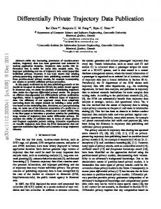
Note that the KL divergence is not available in closed form due to the unknown normalizing constant. Nevertheless, it can be easily computed using the MCMC techniques described in Section 3; see also Handcock et al. (2010) for more details. We use the ergm package (Hunter et al., 2008) in R (R Core Team, 2014) to perform all computations. 4.1. The Lazega Collaboration Network The Lazega dataset records the collaborative working relations between n = 36 partners in a New England firm (Lazega, 2001) and have been analyzed in Snijders et al. (2006) and Hunter and Handcock (2006). Following Handcock et al. (2010), we focus on the undirected network where an edge between two partners exist if they collaborate with each other. The network consists of n = 36 nodes and 115 edges. The network data is supplemented by four attributes: Seniority (the rank number of chronological entry into the firm), Practice (litigation =0 and corporate law = 1), Gender (3 out of the 36 lawyers are female), and Office (three different offices based in three different cities). Figure 1a shows the Lazega network. We consider fitting an ERGM to the Lazega Data with 6 parameters. We add two structural parameters GW ESP and Edges that capture the network structure, two parameters corresponding to the direct effects of Seniority and Practice and three parameters corresponding to the homophily effects of Practice, Gender and Office. The direct effects of seniority and practice are of the following form X xij Zi , i,j
where Zi is the seniority or the practice of partner i. The dyadic homophily effects are given by X xij I(Zi = Zj ) ij
V. Karwa and A. Slavkovi´ c and P. Krivitsky/Sharing Social Network Data]
13
where Zi is the attribute of node i. These terms capture the matches between the two partners on the given attribute and measure the strength of ties between nodes of the same attribute type. Finally, the number structural effect of the network is captured by including the number of edges (density) and a the geometrically weighted edgewise shared partner distributions or GWESP, a measure of transitivity structure in the network, see Snijders et al. (2006). The scale parameter for GWESP term is fixed at its optimal value (0.7781) as described in Hunter and Handcock (2006). This particular form of ERGM was used by Handcock et al. (2010) and an equivalent form was used in Hunter and Handcock (2006). Hunter and Handcock (2006) found that the model provides an adequate fit to the data and can be successfully used to describe the structure of the Lazega dataset, that is explain the observed patterns of collaborative ties as a function of nodal and relational attributes. While there are no obvious privacy concerns in this particular data as with our next study case, one can imagine a scenario where certain partnerships would be exclusive given the nodal information such as gender. Our goal here is to assess the effect of fitting the same model with privacy constraints and evaluate if one can replicate the findings, in particular the parameter estimates, using only synthetic networks released by Algorithm 1. To this end, we release B = 20 synthetic networks using Algorithm 1 and estimate the parameters of the ERGM using the synthetic networks. In Algorithm 1, we set pij = qij = π for all dyads, where π is the probability of retaining an edge (or non-edge). Figure 2 shows plots of 9 such randomly chosen networks for π = 0.98. For understanding the trade-off between risk and utility, we use a range of values of π in Algorithm 1. In particular, we let π, the probability of retaining an edge (in percentage) be 0.1, 0.2, 0.4, 0.5, 1.0, 2.0, 5.0, 10.0, which corresponds to � privacy parameter values of 6.91, 6.21, 5.52, 5.29, 4.60, 3.89, 2.94, 2.20. For estimating the parameters from the synthetic networks, we use two different methods—the naive method which ignores the privacy mechanism and analyzes the synthetic network as is, and our Missing data method that treats the original network as missing. Figure 1b shows the KL divergence between the estimates obtained using the synthetic networks and the estimates from the original network. The x axis denotes the privacy risk as measured by the probability of retaining an edge π. Note that larger values of π imply weaker privacy. The y axis denotes utility of the synthetic networks as measured by the KL divergence on log scale. Smaller values of KL divergence correspond to higher utility. As seen in Figure 1b, the utility of the synthetic networks depends on how they are analyzed. The plot shows that ignoring the privacy mechanism and analyzing the synthetic network leads to a much lower utility. On the other hand, using the missing data method leads to improved utility. Note that since the y axis is in the log scale, as we increase privacy (move from right to left on the x axis) the KL divergence of the naive estimates increases at a much faster rate when compared to the missing data estimates. This is true especially for smaller values of π. Thus for strong privacy protection, the missing data likelihood provides estimates that are closer to the non-private estimates when
V. Karwa and A. Slavkovi´ c and P. Krivitsky/Sharing Social Network Data]
45 43 53 47
43
36
52 38
53 46 41
49
48 46
44
64 59
50
33
49
62 50
34 55
33
56
57 59
38
37
43 39
45
63
67
53
(a) Lazega Dataset
KL Divergence from MLE − Log Scale
factor(Likelihood)
Missing Data
Naive
1e+02 ● ● ●
● ●
1e+00
●
● ●
●
1e−02
●
0.9
0.95
0.98
0.99 0.995 0.996 0.998 0.999
Probability of retaining an edge (b) KL divergence Likelihood
Edges
Missing Data
Naive
gwesp.fixed.0
nodecov.seniority 1e−04
1.00 1.00
0.10 1e−06 0.01 0.01
nodefactor.practice.2
nodematch.gender
nodematch.office
Mean Squared Error
1e−01 1e−02
1e−02
1e−03 1e−03 1e−04 1e−05 1e−04
nodematch.practice
1e−02
1e−04
14
V. Karwa and A. Slavkovi´ c and P. Krivitsky/Sharing Social Network Data]
15
Fig 2: 8 Synthetic copies of the Lazega Network using π = 0.98. The original network is shown in the top left corner in the box and the synthetic networks and original networks are plotted in the same coordinate system for ease of comparison. Notice the addition of fake ties and also removal of existing ties. compared to the naive estimates. Another key feature of the plot is that for any given value of the privacy parameter �, the KL divergence of the missing data estimates has larger variance when compared to the naive estimates, even though the KL divergence of the missing data estimator on an average is smaller than that of the naive estimator. This is actually a feature of the missing data method as it illustrates that the uncertainty should increase when using the
V. Karwa and A. Slavkovi´ c and P. Krivitsky/Sharing Social Network Data]
16
Fig 3: Table showing the parameter estimates based on the original data (MLE) and based on the synthetic networks (Missing and Naive) obtained for the Lazega Data for π = 0.98 Parameter Edges gwesp.fixed.0 nodecov.seniority nodefactor.practice.2 nodematch.gender nodematch.office nodematch.practice
MLE -7.33 1.48 0.04 0.75 0.93 1.41 0.84
Missing Data Estimate MSE -7.32 0.21 1.52 0.2 0.04 0 0.74 0 0.89 0.02 1.4 0.01 0.81 0.01
Bias 0.01 0.03 0 0 -0.04 0 -0.03
Estimate -6.33 0.89 0.03 0.72 0.86 1.32 0.75
Naive MSE 1.1 0.42 0 0 0.02 0.02 0.01
Bias 1 -0.6 0 -0.03 -0.07 -0.09 -0.09
synthetic networks due to the additional source of randomness inherent in the privacy preserving mechanism. The missing data method precisely captures this variation whereas the naive method ignores it. For a more detailed evaluation, let us consider the MSE and the bias (Figure 1c and 1d ) of the both the missing data and naive parameter estimates obtained by using the synthetic networks computed with respect to the estimate obtained from the original data. The plots have two common features. First, in general, as π (probability of retaining an edge) increases, the MSE and the bias are reduced and second, as expected, the estimates based on the missing data method are have smaller bias and MSE than the naive estimates. The MSE and the bias of the naive estimates of the structural parameters are higher when compared to the missing data estimates. The bias for the missing data estimates is always lower than for the naive estimates. However, when π is very close to 1, the MSE of the missing data estimates spikes and is larger than that of the naive estimates. This shows that the variance of the missing data estimates is much larger for values of π close to 1. When π is very close to 1, the synthetic network is not very different from the original network, hence the noise due to the MCMC estimation in missing data method increases the variance. Table 3 shows the parameter estimates, bias and the mean squared error of the estimates obtained by using synthetic networks generated by setting π = 0.98, which corresponds to an � = 3.89. The table shows that the missing data estimates have a very small empirical bias , i.e. they are close to the maximum likelihood estimates based on the original network. On the other hand, the bias and MSE of the naive estimates obtained by ignoring the privacy mechanism are larger. Note that the estimates of the structural parameters and the homophily effects are more biased when compared to the main effects of the nodes. The results of this case study show that we can replicate the analysis using synthetic networks, but we need to model the mechanism that generated the network explicitly and use the missing data likelihood. For extremely small values of perturbing an edge (e.g., 1 − π), it appears that the missing data estimates only increase the variance, as the estimates are already unbiased and close to the MLE.
V. Karwa and A. Slavkovi´ c and P. Krivitsky/Sharing Social Network Data]
17
4.2. Teenage friendship and substance use data For the second case study, we use the teenage friendship network which is a part of the data collected in the Teenage Friends and Lifestyle Study (Michell and Amos, 1997; Pearson and Michell, 2000). The study records a network of friendships and substance use for a cohort of students in a school in Scotland. We used an excerpt of 50 adolescent girls made available online in the Siena package (Siena, 2014). The network consists of 50 nodes and 39 edges. There are four covariates associated with each node: Drug usage (yes or no), Smoking status (yes or no), Alcohol usage, (regular or irregular) and Sport activity (regular or irregular). Figure 4a shows the friendship network along with the drug usage. As before, we assume that the attributes associated with each node are available publicly. Our goal is to protect the relationship information in the network and study how one can replicate the analysis on the original network by fitting an ERGM to differentially private synthetic networks. We fit an ERGM with 6 terms, as shown in equation 6 below. Pθ (X) ∝ exp{θ1 edges + θ2 gwesp + θ3 popularity + θ4 drug + θ5 sport + θ6 smoke}. (6) As explained in section 4.1, the first three terms in equation 6 capture the network structure of the graph, and the last three terms represent the homophily effect of covariates. The term edges measures the number of edges in the network. The term gwesp measures the transitive effects in the network, and the term popularity captures the degree distribution of the network. The remaining three terms measure the homophily effects of drug usage, involvement in sports and the smoking behavior. For this case study, we also consider two different methods for releasing synthetic networks. In particular, we allow different privacy risks for different types of edges. Such a strategy is useful when it is believed that revealing certain types of ties, given the nodal information, will have higher privacy risks associated with them. The choice of which ties are riskier if revealed of course depends on the application. In this case study, we deem ties involving nodes that use drugs riskier than other ties, and hence provide more privacy protection to such ties. In the first method, we assume that the privacy risk of a dyad depends on the node attributes and accordingly we let the probability of retaining an edge depend on the attributes of nodes. More concretely, we use two different values for the probability of retaining an edge: π1 = 0.62 and π2 = 0.88, corresponding to the privacy risk as measured by � equal to 0.5 and 2, respectively. We set pij = π1 if both nodes i and j use drugs, otherwise we set pij = π1 . The overall privacy risk for any dyad as measured by � is governed by π2 and is equal to 2 (high privacy risk). However, the privacy risk for dyads between nodes that use drugs is 0.5 (low privacy risk) and hence the privacy protection for dyads between nodes that use drugs is higher. We compare this network release strategy with two other strategies where all dyads are released either with π = π1 or with π = π2 . Figure 5 shows the utility (as measured by KL
V. Karwa and A. Slavkovi´ c and P. Krivitsky/Sharing Social Network Data]
18
(a) Teenage Friendship Data factor(Likelihood)
Missing Data
Naive
Likelihood
Missing Data
Naive
Edges
Gwesp
nodematch.drug.0
●
10.0
1.00
1.0
1.00
100
0.10
●
0.10 0.1
0.1 ●
0.01 0.01
●
nodematch.drug.1
nodematch.smoke.0
nodematch.smoke.1
0.100
●
nodematch.sport.0 0.100
Mean Squared Error
0.10 ●
●
0.10
0.010
0.010 0.01
0.01
1
0.001
0.001
● ●
● ●
nodematch.sport.1
nodematch.sport.alcohol 1.00
● ● ● ●
0.10 0.10 ● ●
0.9
0.95
0.98
0.01
0.99 0.995 0.996 0.998 0.999 0.01
0.900 0.925 0.950 0.975 1.000
0.900 0.925 0.950 0.975 1.000
Probability of retaining an edge (b) KL divergence
Degree Popularity
1000
● ●
●
● ●
●
● ●● ● ● ● ● ●
100
● ● ●
10
●
●
10
● ● ● nodematch.sport.1
10
● ● ● ●
●
● ● ● ●●
● ●
1000
● 100
● ● ● ● ● ● nodematch.sport.alcohol
● ● ● ● ● ● ● ● ● ● ● ●
nodematch.sport.0
● ●
100
1
100
nodematch.smoke.1
●
● ●
● ● ● ● ● ●● ● ● ●
10
1000
● ●
● ●● ● ● ● ●
●
●
1000
100
nodematch.drug.0
● 1000
●
1000
nodematch.smoke.0
● ●
Naive
●
●● ● ● ● ● ● ● ● ● ●
nodematch.drug.1
●
●
●
Gwesp
● 1000
●
10
Missing Data
Edges
●
100
● ●
Probability of retaining an edge
(c) Mean Squared Error
Likelihood
Percentage Absolute Bias
KL Divergence from MLE − Log Scale
Degree Popularity
● ●● ● ● ●
100
● ● ●
10
● ● ● ● ●
● ●● ● ● ● ●
10
● ● ●
KL Divergence from MLE
V. Karwa and A. Slavkovi´ c and P. Krivitsky/Sharing Social Network Data]
factor(Likelihood)
Missing Data
19
Naive
1000
100
0.62 and 0.88
0.62
0.88
Probability of retaining an edge Fig 5: Box plots of utility when privacy risks depend on the node attributes. divergence) for these three synthetic network strategies. We can see that the utility is lowest when we use probability of π = 0.62 which corresponds to the lowest privacy risk. However, if we increase the privacy risks for dyads between nodes that do not use drugs, we get an improved utility. Finally, if we increase the privacy risk for all dyads (π = 0.62), we get much higher utility, but at the expense of reduced privacy. In the second method, the privacy risk for every dyad is assumed to be the same and we set pij = qij = π for each dyad. Figure 6 shows 9 synthetic networks generated using π = 0.98. As before, to study the trade-offs between risk and utility, we let π vary (in percentage) in the set 0.1, 0.2, 0.4, 0.5, 1.0, 2.0, 5.0, 10.0 and use KL divergence, MSE and bias to evaluate the utility. Figures 4b, 4c and 4d show the results. In particular, Figure 4b shows that the KL divergence between the private estimate and the non-private estimate increases as π increases, thus stronger privacy leads to reduced utility. However, the KL divergence of the naive likelihood increases at a much faster rate when compared to the missing data likelihood. This is true especially for larger values of π. Thus for strong privacy protection, the missing data likelihood provides estimates that are closer to the non-private estimates when compared to the naive likelihood. Figures 4c and 4d show the mean squared error and the percentage absolute bias of the parameter estimates for the Teenage Dataset. The results are very similar to those obtained in the Lazega case study shown in Section 4.1. A few notable differences between the teenage dataset and the Lazega dataset is the computed MSE and bias in the structural parameters, GWESP, degree popularity and the number of edges. In the Teenage data, the improvement in bias and the MSE of the structural parameters by using the missing data likelihood method is not as high as the improvement obtained in the Lazega
V. Karwa and A. Slavkovi´ c and P. Krivitsky/Sharing Social Network Data]
20
Fig 6: 8 Synthetic copies of the Teenage Friendship Network using π = 0.98. The original network is shown in the top left corner in the box and the synthetic networks and original networks are plotted in the same coordinate system for ease of comparison. Notice the addition of fake ties and also removal of existing ties. data. This is due to the fact that the Teenage data are much sparser when compared to the Lazega dataset. Table 7 shows the parameter estimates for p = 0.98, along with the bias and the MSE. We can see that the bias of the missing data estimates is smaller than the bias of the naive estimates. However, the MSE of the missing data estimates in some cases is larger than the MSE of the naive estimates. This is expected as the missing data estimates take into account the additional uncertain in the privacy mechanism. 5. Conclusion Motivated by a growing availability of network data combined with growing concerns about privacy, we described a framework for sharing relational data that not only preserves the privacy of individual relationships in a quantifi-
V. Karwa and A. Slavkovi´ c and P. Krivitsky/Sharing Social Network Data]
21
Fig 7: Table showing the parameter estimates based on the original data (MLE) and based on the synthetic networks (Missing and Naive) obtained for the Teenage Friendship Data for π = 0.98 Parameter Degree Popularity Edges gwesp.fixed.0 nodematch.drug.0 nodematch.drug.1 nodematch.smoke.0 nodematch.smoke.1 nodematch.sport.0 nodematch.sport.1 nodematch.sport.alcohol
MLE -1.9 2.09 1.5 1.57 0.81 -0.4 0.95 0.53 -0.73 1.31
Missing Data estimate mse bias -1.5 0.36 0.4 1.09 4.35 -0.99 1.35 0.08 -0.15 1.74 0.28 0.17 0.86 0.2 0.05 -0.57 0.22 -0.16 0.84 0.26 -0.11 0.36 0.49 -0.17 -1.11 0.52 -0.38 1.42 0.17 0.1
Naive Data estimate mse -0.83 1.2 0.06 5.38 0.6 0.82 0.97 0.47 0.73 0.06 -0.11 0.19 0.56 0.26 0.47 0.2 -0.42 0.29 0.83 0.28
bias 1.07 -2.02 -0.9 -0.59 -0.08 0.3 -0.4 -0.06 0.3 -0.48
able manner, but also allows meaningful inferences by making efficient use of it in estimating the popular exponential-family random graph models. As is, the framework can be used for replication of statistical analyses, but for larger networks, the loss of precision due to the added noise is likely to become negligible as well. Randomized response scheme we propose is simple yet effective, and quantifiable via the Edge Differential Privacy framework that measures privacy risk in terms of a worst case disclosure. We performed two case studies to evaluate how well the proposed approach works at a variety of privacy levels, and demonstrate its usefulness in addressing the realistic challenge of simultaneously maintaining the privacy of sensitive relations in the network and sharing of the network data that would support valid statistical inference. Our analyses show that the proposed approach leads to estimates much closer to those obtained for a full network than those obtained by ignoring the privacy mechanism. We can replicate the original analyses using synthetic networks, but we need to model the mechanism that generated the network explicitly and use the missing data likelihood. Although we advocate the use of missing data and MCMC techniques by analysts who use data obtained from a differentially private mechanism, or more general privacy-preserving mechanisms, they can also be used by data curators to release synthetic graphs for performing preliminary analysis of other models. A key advantage of this method in relation to other proposed methods for private release of ERGMs is that the released private synthetic graphs preserve the actual relations and not just sufficient statistics, so our technique allows us to find MLE of any ERGM that could have been fitted to the original network, at a modest computational cost. In particular, an exchange algorithm requires an MCMC sample of network realizations for each MCMC draw of θ from the posterior—MCMC within MCMC—which vastly increases the computational cost, when our approach merely doubles it, with the two samples able to be run in parallel.
V. Karwa and A. Slavkovi´ c and P. Krivitsky/Sharing Social Network Data]
22
In addition, having estimated θˆy from the perturbed graph, we can simulate from the conditional distribution X|θˆy , y (∝ Pγ (Y = y|X = x)Pθ (X = x)): possible graphs x from which y could have plausibly come. For example, if x exhibited strong homophily on some actor attribute, y, which has had false ties added at random, would exhibit weaker homophily. The amount of homophily in x could be estimated by the ERGM using our technique, and graphs simulated from X|θˆy , y would retain most of the relations in y, but “clean” many of the false ties inconsistent with the model. We have used differential privacy as our measure of protection, but this approach, while it provides strong guarantees has substantive limitations. For example, we distinguished 1 − pij , the probability of hiding a tie, from 1 − qij , the probability of creating a false tie. Our inferential framework handles this seamlessly, and this distinction is important if the ties reflect socially or legally stigmatized relationships. In that case, one might want to set 1 − qij to a relatively high value in order to create deniability for actors with such relationships. But, setting 1 − pij > 0 would reduce utility to little gain to privacy in practice. Therefore, one might set pij = 1, but then Proposition 1 gives � = ∞. This suggests that this measure is too crude to assess disclosure risk when there is an assymmetry in the consequences of a tie as opposed to a non-tie being exposed. We assumed that the covariate information is available publicly, which may not always be the case. We are currently working on relaxing this assumption and releasing synthetic graphs that protect both nodal and structural information in a graph. Future investigations will also include evaluating the usefulness of this approach for different sizes and sparsity of networks and other ERGM specifications. Lastly, we assume that while the relationships are sensitive, the exogenous individual attributes such as gender are not: they can be released completely and without noise. This is a limitation inherent in ERGMs, which treat them as fixed and known covariates. The exponential-family random network models (ERNMs) introduced by (Fellows and Handcock, 2012) propose to model relations and actor attributes jointly in an exponential family framework. If actor attributes are perturbed as well with a known probability, our inferential approach should be directly applicable. Acknowledgments. This work was supported in part by NSF grant BCS-0941553 to the Department of Statistics, Pennsylvania State University and by the Singapore National Research Foundation under its International Research Centre @ Singapore Funding Initiative and administered by the IDM Programme Office, Media Development Authority (MDA). References Backstrom, L., Dwork, C. and Kleinberg, J. (2007). Wherefore art thou r3579x?: anonymized social networks, hidden patterns, and structural
V. Karwa and A. Slavkovi´ c and P. Krivitsky/Sharing Social Network Data]
23
steganography. In Proceedings of the 16th international conference on World Wide Web 181–190. ACM. Bearman, P. S., Moody, J. and Stovel, K. (2004). Chains of Affection: The Structure of Adolescent Romantic and Sexual Networks1. American Journal of Sociology 110 44–91. Carroll, R. J., Ruppert, D., Stefanski, L. A. and Crainiceanu, C. M. (2012). Measurement error in nonlinear models: a modern perspective. CRC press. Chaudhuri, A. (1987). Randomized Response: Theory and Techniques. Statistics: A Series of Textbooks and Monographs. CRC Press. Dwork, C., McSherry, F., Nissim, K. and Smith, A. (2006a). Calibrating noise to sensitivity in private data analysis. In TCC 265–284. Springer. Dwork, C., Kenthapadi, K., McSherry, F., Mironov, I. and Naor, M. (2006b). Our Data, Ourselves: Privacy Via Distributed Noise Generation. In EUROCRYPT. LNCS 486-503. Springer. Fellows, I. and Handcock, M. S. (2012). Exponential-family Random Network Models. arXiv preprint arXiv:1208.0121. Fienberg, S. E., Rinaldo, A. and Yang, X. (2010). Differential privacy and the risk-utility tradeoff for multi-dimensional contingency tables. In Proceedings of the 2010 international conference on Privacy in statistical databases. PSD’10 187–199. Springer-Verlag, Berlin, Heidelberg. ´, A. B. (2010). Data Privacy and ConfidenFienberg, S. E. and Slavkovic tiality. International Encyclopedia of Statistical Science 342-345. SpringerVerlag. Geyer, C. J. and Thompson, E. A. (1992). Constrained Monte Carlo maximum likelihood for dependent data (with discussion). Journal of the Royal Statistical Society. Series B. Methodological 54 657–699. Goldenberg, A., Zheng, A. X., Fienberg, S. E. and Airoldi, E. M. (2010). A survey of statistical network models. Foundations and Trends in Machine Learning 2 129–233. Goodreau, S. M., Kitts, J. A. and Morris, M. (2009). Birds of a feather, or friend of a friend? using exponential random graph models to investigate adolescent social networks. Demography 46 103–125. Handcock, M. S. (2003). Statistical models for social networks: Inference and degeneracy. Dynamic social network modeling and analysis 126 229–252. Handcock, M. S., Gile, K. J. et al. (2010). Modeling social networks from sampled data. The Annals of Applied Statistics 4 5–25. Handcock, M. S., Hunter, D. R., Butts, C. T., Goodreau, S. M., Krivitsky, P. N. and Morris, M. (2015). ergm: Fit, Simulate and Diagnose Exponential-Family Models for Networks The Statnet Project (http: //www.statnet.org) R package version 3.4. Hay, M., Li, C., Miklau, G. and Jensen, D. (2009). Accurate estimation of the degree distribution of private networks. In Data Mining, 2009. ICDM’09. Ninth IEEE International Conference on 169–178. IEEE. Hout, A. and Heijden, P. G. (2002). Randomized Response, Statistical Disclosure Control and Misclassificatio: a Review. International Statistical Re-
V. Karwa and A. Slavkovi´ c and P. Krivitsky/Sharing Social Network Data]
24
view 70 269–288. Hundepool, A., Domingo-Ferrer, J., Franconi, L., Giessing, S., Nordholt, E. S., Spicer, K. and De Wolf, P.-P. (2012). Statistical disclosure control. Wiley. com. Hunter, D. R., Goodreau, S. M. and Handcock, M. S. (2008). Goodness of Fit of Social Network Models. Journal of the American Statistical Association 103 248-258. Hunter, D. R. and Handcock, M. S. (2006). Inference in curved exponential family models for networks. Journal of Computational and Graphical Statistics 15. Hunter, D. R., Handcock, M. S., Butts, C. T., Goodreau, S. M. and Morris, M. (2008). ergm: A package to fit, simulate and diagnose exponential-family models for networks. Journal of Statistical Software 24 nihpa54860. Karwa, V. and Slavkovic, A. B. (2012). Differentially Private Graphical Degree Sequences and Synthetic Graphs. In Privacy in Statistical Databases, (J. Domingo-Ferrer and I. Tinnirello, eds.). Lecture Notes in Computer Science 7556 273-285. Springer Berlin Heidelberg. ´, A. B. and Krivitsky, P. (2014). Differentially Karwa, V., Slavkovic Private Exponential Random Graphs. In Privacy in Statistical Databases (J. Domingo-Ferrer, ed.). Lecture Notes in Computer Science 8744 143– 155. Springer International Publishing. ´, A. B. (2015). Inference using noisy degrees: DifKarwa, V. and Slavkovic ferentially Private β-model and synthetic graphs. The Annals of Statistics. Karwa, V., Raskhodnikova, S., Smith, A. and Yaroslavtsev, G. (2011). Private Analysis of Graph Structure. Proceedings of the VLDB Endowment 4. Lazega, E. (2001). The collegial phenomenon: The social mechanisms of cooperation among peers in a corporate law partnership. Oxford University Press. Lu, W. and Miklau, G. (2014). Exponential Random Graph Estimation Under Differential Privacy. In Proceedings of the 20th ACM SIGKDD International Conference on Knowledge Discovery and Data Mining. KDD ’14 921–930. ACM, New York, NY, USA. Michell, L. and Amos, A. (1997). Girls, pecking order and smoking. Social Science & Medicine 44 1861–1869. Morris, M., Handcock, M. S. and Hunter, D. R. (2008). Specification of exponential-family random graph models: terms and computational aspects. Journal of statistical software 24 1548. Narayanan, A. and Shmatikov, V. (2009). De-anonymizing social networks. In Security and Privacy, 2009 30th IEEE Symposium on 173–187. IEEE. Nissim, K., Raskhodnikova, S. and Smith, A. (2007). Smooth sensitivity and sampling in private data analysis. In STOC 75–84. ACM. Pearson, M. and Michell, L. (2000). Smoke rings: social network analysis of friendship groups, smoking and drug-taking. Drugs: Education, Prevention and Policy 7 21–37. Robins, G., Pattison, P., Kalish, Y. and Lusher, D. (2007). An introduc-
V. Karwa and A. Slavkovi´ c and P. Krivitsky/Sharing Social Network Data]
25
tion to exponential random graph models for social networks. Social networks 29 173–191. Siena (2014). Description excerpt of 50 girls from “Teenage Friends and Lifestyle Study” data. http://www.stats.ox.ac.uk/~snijders/siena/ s50_data.htm/. Snijders, T. A. (2002). Markov chain Monte Carlo estimation of exponential random graph models. Journal of Social Structure 3 1–40. Snijders, T. A., Pattison, P. E., Robins, G. L. and Handcock, M. S. (2006). New specifications for exponential random graph models. Sociological methodology 36 99–153. R Core Team (2014). R: A Language and Environment for Statistical Computing R Foundation for Statistical Computing, Vienna, Austria. Wasserman, S. S. and Pattison, P. (1996). Logit Models and Logistic Regressions for Social Networks: I. An Introduction to Markov Graphs and p∗ . Psychometrika 61 401–425. Wasserman, L. and Zhou, S. (2010). A statistical framework for differential privacy. J. Amer. Statist. Assoc. 105 375–389. MR2656057 (2011d:62015) ´, A. B. (2012). Logistic regression with Woo, Y. M. J. and Slavkovic variables subject to post randomization method. In Privacy in Statistical Databases 116–130. Springer.