Sharp-interface nematic-isotropic phase transitions without flow - Core

Sharp-interface nematic-isotropic phase transitions without flow Paolo Cermelli,∗ Eliot Fried† and Morton E. Gurtin‡ ∗

†

Dipartimento di Matematica Universit` a di Torino Via Carlo Alberto 10 10123 Torino, Italy

Department of Mechanical Engineering Washington University in St. Louis St. Louis, MO 63130-4899, USA

‡

Department of Mathematical Sciences Carnegie Mellon University Pittsburgh, PA 15213-3190, USA

Abstract We derive a supplemental evolution equation for an interface between the nematic and isotropic phases of a liquid crystal when flow is neglected. Our approach is based on the notion of configurational force. As an application, we study the behavior a spherical isotropic drop surrounded by a radially-oriented nematic phase: our supplemental evolution equation then reduces to a simple ordinary differential equation admitting a closed form solution. In addition to describing many features of isotropic-to-nematic phase transitions, this simplified model yields insight concerning the occurrence and stability of isotropic cores for hedgehog defects in liquid crystals.

1

Introduction

When quenched from a high-temperature isotropic phase to a low-temperature nematic phase, a liquid crystal undergoes a first-order phase transition (de Gennes 1971). Such transitions proceed via the nucleation, growth, and coalescence of droplets (Ostner, Chan & Kahlweit 1973). Experiments involving free- and directional-growth show that nematic-isotropic phase interfaces exhibit a host of interesting morphological instabilities, instabilities that are manifested by the formation of dendrites (Armitage & Price 1978) and periodic cellular patterns (Oswald, Bechoeffer & Libchaber 1987) resembling those occuring in crystal growth (Langer 1980). Here, we take a first step toward developing a sharp-interface theory for the description of such phenomena. Our goal is a generalization of the Ericksen–Leslie theory (Ericksen 1961; Leslie 1968) for uniaxial nematics which • allows for phase transitions, • models an nematic-isotropic interfaces as a sharp surface across which bulk fields may suffer discontinuities, • accounts for localized interactions between phases by endowing the interface with excess properties.

2

P. Cermelli, E. Fried & M. E. Gurtin

Our work is a first step because, for clarity, we neglect effects associated with flow and with heat and mass transport. Hence, what we present is in essence a generalization of the classical curvature elasticity theory (Oseen 1933; Z¨ocher 1933; Frank 1958). As we neglect flow and both thermal and compositional influences, the free-energy (density) of the isotropic phase is a constant that, without loss in generality, we set equal to zero. This allows us to restrict attention to the nematic phase and the nematicisotropic interface. Our discussion begins with a concise overview of the theory for the nematic phase. In addition to a director momentum balance, that theory is based an isothermal statement of the second law that is used to restrict constitutive equations. To deal with the nematic-isotropic interface, we rely on recent developments in the theory of configurational forces (Gurtin 1995, 2000; Gurtin & Struthers 1990). Although configurational forces are superfluous away from the interface, the interfacial limits of the bulk configurational stress and configurational momentum are of essential importance. Prior to considering the interface, we therefore reformulate the theory for the nematic phase in a manner that accounts for the role of configurational forces. Using control volumes that migrate within the nematic phase this yields representations for the configurational stress and momentum in bulk, representations obtained without recourse to constitutive assumptions and, hence, more broadly valid than would be counterparts derived on the basis of variational arguments (Maugin & Trimarco 1995). Our treatment of the interface is analogous to that taken in our reformulation of the bulk theory. Aside from the director momentum balance, we impose a configurational momentum balance and an isothermal version of the second law that accounts for power expended by both the director and configurational forces. As in the theory for the nematic phase, the interfacial dissipation inequality is used to obtain restrictions on constitutive equations. With those restrictions, we arrive at the general system of evolution equations for the interface. Those equations, which enforce the director momentum balance and the normal component of the configurational momentum balance, supplement the bulk director momentum balance arising from the standard theory. ˆ Precisely, denote by n the director, let G = grad n, and let Ψ(n, G) denote the bulk free energy. The evolution equation in the nematic phase in the absence of flow is classical:  ˆ  ˆ ˆ ∂Ψ ∂Ψ ∂Ψ ˙ 2 n) + γ n˙ = div σ(¨ n + |n| + G: n− , (1.1) ∂G ∂G ∂n with σ > 0 the director mass density and γ ≥ 0 a viscosity associated with changes in director-orientation. The conditions at a stationary nematic-isotropic interface are also classical, and involve an interfacial free energy (density) ψ to describe weak anchoring (Rapini & Papoular 1969) and a dissipative contribution (Derzhanski & Petrov 1979): denoting by m the unit interfacial normal directed away from the nematic phase and by ◦ n the normal-time derivative of n, our generalization of the Derzhanski–Petrov condition ˆ m) and takes the form to an evolving interface has ψ = ψ(n, ◦

β1 n + σV n˙ = −

ˆ ∂Ψ ∂ ψˆ , m− ∂G ∂n

(1.2)

with β1 ≥ 0 a dissipative coefficient. The configurational balance provides the evolution equation for the phase interface. Denoting by V the normal velocity of the interface, by K its total curvature (twice the mean curvature) and by divS the surface divergence, we obtain the evolution equation  ˆ ∂ψ ∂ ψˆ ◦ ◦ ˙ 2 ). (1.3) β1 Gm · n + divS (β2 m) + β3 V = ψK − divS − Gm · − (Ψ − 12 σ|n| ∂m ∂n

Sharp-interface nematic-isotropic phase transitions without flow

3

with β2 ≥ 0 and β3 ≥ 0 additional dissipative coefficients. To our knowledge this equation has never been proposed in the literature. However, our developments complement recent work (Poniewierski 2000; Rey 2000a, b, c, 2001; Cheong & Rey 2002) concerning the rheology of a material interface between a nematic liquid crystal and an isotropic fluid. We specialize (1.3) to two simple applications. In the first we develop approximate equations for a perturbed planar interface S0 such that m

= e + m1 + o(),

V = V0 + V1 + o(),

n = e + n1 + o(),

(1.4)

with e a fixed unit vector and  a small parameter. The simplest such equations arise for ˆ m) = ψ0 and Ψ = Ψ0 + Ψ1 + o(), with ψ0 , Ψ0 and Ψ1 given constants. Then, with ψ(n, β2 constant and inertia neglected, (1.3) is approximated, at the zeroth and first order in , by β3 V0 = −Ψ0 ,

◦

−β2 K 1 + β3 V1 = ψ0 K1 − Ψ1 ,

(1.5)

the second of which, for β2 = 0, is the classical curvature-flow equation (cf., e.g., Gurtin 2000). As a second application, we discuss the growth and equilibrium of a spherical isotropic drop in a nematic ocean in which the director is radially oriented. The evolution equation (1.3) then reduces to the ordinary differential equation κ 2σ β R˙ = Ψ0 − + 2 R R

(1.6)

for the radius R of the isotropic drop. The moduli σ > 0 and κ > 0 are related to surface energy and bulk elasticity, while Ψ0 is a measure of the bulk energy difference between the phases, and possibly depends on temperature. The solutions of (1.6) have different behavior according to the size and sign of the nematic-isotropic energy difference Ψ0 . When Ψ0 ≤ 0, so that the energy of the nematic phase is lower than that of the isotropic phase, (1.6) has a stable equilibrium R∗ . Hence, an isotropic drop in a nematic ocean is stable at the characteristic radius R∗ , a fact that might explain the presence of an isotropic core for hedgehog defects: our theory indeed allows for an estimate of the core radius. When 0 < Ψ0 < σ 2 /κ, so that the nematic phase has the higher energy, (1.6) still has a stable equilibrium R∗− , but also has an unstable equilibrium R∗+ > R∗− : in this regime the surface tension σ is sufficiently large compared to Ψ0 , so that small isotropic droplets persist in the nematic phase. However, if the radius of the drop is large enough, the drop grows and the nematic phase eventually becomes isotropic. This result is consistent with observations showing that, for the phase transformation proceed beyond a certain stage, isotropic nuclei must coalesce. Finally, when Ψ0 ≥ σ 2 /κ, so that the energy difference between the nematic and isotropic phase is sufficiently large, (1.6) has no equilibrium points and the isotropic phase grows at the expense of the nematic phase.

2

Theory for the nematic phase

Throughout this section P denotes an arbitrary (fixed) region lying within the nematic phase. Our developments can be viewed as a specialization of the Ericksen–Leslie theory (Ericksen 1961; Leslie 1968) that neglects flow and thermal transport.

4

2.1

P. Cermelli, E. Fried & M. E. Gurtin

Kinematics

We write n(x, t) for the director field, assumed consistent with the constraint |n| = 1.

(2.1)

Using grad to denote the gradient operator, we write G = grad n

(2.2)

for the director gradient; then, by (2.1), Gn = 0.

(2.3)

We use a superposed dot to denote time-differentiation, so that, ˙ = 0. n·n

2.2

(2.4)

Balance of director momentum

We write σ for the (constant) director mass density (i.e., the peculiar mass density of the mesogens), r = σ n˙

(2.5)

for the director momentum (density), S for the director stress, and g for the director body force (density). Balance of director momentum requires that, for any P,  ˙   r dv = Sm∂P da + g dv, P

(2.6)

P

∂P

or, equivalently, that the field equation r˙ = div S + g

(2.7)

hold throughout the nematic phase. A direct calculation allows us to decompose (2.7) into components, ˙ = div (S − n⊗Sn) + GSn + (G : S)n + g − (g·n)n, r˙ − (r· n)n r˙ ·n = div (Sn) − G : S + g·n,

 (2.8)

perpendicular and parallel to the director.

2.3

Energy imbalance

We restrict attention to isothermal processes, in which case the first and second laws of thermodynamics reduce to an imbalance of energy asserting that, for any P, the net (free plus kinetic) energy of P change at a rate that is not greater than the power expended on P. Writing Ψ for the free-energy (density), so that Ψ + 12 r·n˙ represents the net energy per unit volume, and noting that ∂P Sm∂P · n˙ da represents the power expended on P by material exterior to P, the energy imbalance requires that .   ˙ dv ≤ (Ψ + 12 r· n) P

Sm∂P · n˙ da. ∂P

(2.9)

Sharp-interface nematic-isotropic phase transitions without flow

5

Using the balance of director momentum, (2.7), we may write (2.9) equivalently as  ˙ + g· n) ˙ − S: G ˙ dv ≤ 0. (Ψ

(2.10)

P

The requirement that (2.10) hold for all P is therefore equivalent to the requirement that the dissipation inequality ˙ + g· n˙ ≤ 0 ˙ − S: G Ψ

(2.11)

hold throughout the nematic phase.

2.4

Constitutive equations

We take Ψ to be given constitutively as a function ˆ Ψ = Ψ(n, G).

(2.12)

 ˆ   ˆ  ∂ Ψ(n, G) ∂ Ψ(n, G) ˙ − S :G + + g · n˙ ≤ 0. ∂G ∂n

(2.13)

Then (2.11) takes the form

Constitutive equations for S and g that ensure satisfaction of the dissipation inequality (2.11) are given by  ˆ  ∂ Ψ(n, G)   S = n⊗α + ,  ∂G  ˆ  ∂ Ψ(n, G)  ˙  g = λn − Gα − − γ(n, G)n, ∂n

(2.14)

with γ ≥ 0 and with α and λ constitutively indeterminate fields that arise in response to the constraint (2.1),1 where differentiation is performed on the manifold defined by  ˆ ˆ (2.1), so that (∂ Ψ/∂G) n = 0 and (∂ Ψ/∂n)·n = 0.

2.5

Basic partial differential equation in the nematic phase

If we combine the balance (2.8)1 and the constitutive equations (2.14), we arrive at the partial differential equation that governs the evolution of the director in the nematic phase:

 ¨ − |n| ˙ 2 n + γ n˙ = div σ n

 ˆ  ˆ ˆ ∂Ψ ∂Ψ ∂Ψ + G: n− . ∂G ∂G ∂n

(2.15)

We refer to (2.15) as the (constitutively augemented) director momentum balance in bulk. 1 We avoid a detailed discussion of constraints and associated multiplier fields. A modern geometrical treatment of constraints in a material with nematic microstructure is given by Anderson, Carlson & Fried (1999).

6

3

P. Cermelli, E. Fried & M. E. Gurtin

Configurational forces and configurational momentum in the nematic phase

The goal of this study is a complete theory of nematic-isotropic transitions in which the interface is allowed to move relative to the material. In variational treatments of related equilibrium problems, independent kinematical quantities may be independently varied, and each such variation yields a corresponding Euler–Lagrange balance. In dynamics with general forms of dissipation there is no encompassing variational principle, but experience has demonstrated the need for an additional balance associated with the kinematics of the interface. Here, guided by variational treatments in which such a balance is a consequence of the assumption of equilibrium, we follow Gurtin & Struthers (1990) and Gurtin (1995, 2000) and introduce, as primitive objects, configurational forces and momentum together with an independent balance of configurational momentum. Roughly speaking, configurational forces are related to the integrity of the material structure and expend power in the transfer of material and in the evolution of the interface. In this part we discuss configurational forces in bulk. Within that context such forces are extraneous to the solution of actual boundary-value problems. But in general situations knowledge of the structure of configurational forces in bulk away from the interface is central to the understanding of their localized behavior at the interface.

3.1

Balance of configurational momentum

We consider a configurational momentum balance involving three fields: a configurational momentum (density) q, a configurational stress C, and a configurational body force (density) f . Balance of configurational momentum then requires that, for any P,  ˙   q dv = Cm∂P da + f dv, P

∂P

(3.1)

P

or, equivalently, that the field equation q˙ = div C + f

(3.2)

hold throughout the liquid.

3.2

Migrating control volumes. Observed and relative velocities

To characterize the manner in which configurational forces perform work, a means of capturing the kinematics associated with the transfer of material is needed. Following Gurtin (1995, 2000), we accomplish this with the aid of control volumes R(t) that migrate relative to the liquid and thereby result in the transfer of material to — and the removal of material from — R(t) at ∂R(t). Here it is essential that fixed regions P not be confused with control volumes R(t) that migrate relative to the material. The use of migrating control volumes allows us to determine representations for the configurational stresses and momenta in bulk. Let R = R(t) be a migrating control volume with V∂R (x, t) the (scalar) normal velocity of ∂R(t) in the direction of the outward unit normal m∂R (x, t). To describe power expenditures associated with the migration of R(t), we introduce a field v∂R (x, t) defined over ∂R(t) for all t. Compatibility then requires that v∂R have V∂R as its normal component, v∂R ·m∂R = V∂R ,

(3.3)

Sharp-interface nematic-isotropic phase transitions without flow

7

but v∂R is otherwise arbitrary. We refer to any such field v∂R as a velocity field for ∂R. Nonnormal velocity fields, while not intrinsic, are important. For example, given an ˆ (ξ1 , ξ2 , t) of ∂R, the field defined by arbitrary time-dependent parametrization x = x ˆ /∂t (holding (ξ1 , ξ2 ) fixed) generally represents a nonnormal velocity field for v∂R = ∂ x ∂R. But while it is important that we allow for the use of non-normal velocity fields, it is essential that the theory itself not depend on the particular velocity field used to describe a given migrating control volume. As we shall see, this observation has important consequences. We refer to the normal velocity V∂R and any choice of the velocity field v∂R for ∂R as migrational velocities for ∂R. Given a migrating control volume R, the field n˙ + Gv∂R

(3.4)

represents the rate of change of the director following the migration of ∂R. Useful in what follows is the following transport identity: given a smooth field Φ(x, t) and a migrating control volume R = R(t),  ˙   ˙ Φ dv = Φ dv + ΦV∂R da. R

3.3 3.3.1

R

(3.5)

∂R

Expended power Power expended by tractions

The conventional form for the power expended by material exterior to a fixed region P is Sm∂P ·n˙ da. Consider, instead, a migrating control volume R = R(t). The migration ∂P of R involves a transfer of material across ∂R and we expect that this transfer should be accompanied by a power expenditure over and above the conventional expenditure. Configurational forces are introduced to account for power expenditures associated with material transfer. Specifically, we view the configurational traction Cm∂R distributed over ∂R as a force, per unit area, associated with the transfer of material across ∂R. Since any velocity field v∂R for ∂R represents the velocity with which material is transferred across ∂R, we take v∂R to be an appropriate power-conjugate velocity for Cm∂R , and hence assume that the migration of R is accompanied by the power expenditure Cm∂R ·v∂R da. ∂R We assume that the velocity power-conjugate to the director traction Sm∂R is not ˙ but rather by n˙ + Gv∂R , the given by n,  rate of change of the director following the migration of ∂R (cf. (3.4)); granted this, ∂R Sm∂R ·(n˙ + Gv∂R ) da represents the power expended on ∂R by the director traction. Material is added to R only along its boundary ∂R; there is no transfer of material to the interior of R. For that reason, the configurational body force f expends no power. The total power expended on R by tractions over ∂R is therefore given by  W (R) = ∂R

 Sm∂R ·(n˙ + Gv∂R ) + Cm∂R ·v∂R da.

(3.6)

8

P. Cermelli, E. Fried & M. E. Gurtin

3.3.2

Momentum forces and their associated power expenditures

The momentum balance (3.1), written for a migrating control volume R, takes the form   ˙      r dv = Sm∂R da + g dv + rV∂R da,      R R ∂R ∂R (3.7)  ˙        q dv = Cm∂R da + f dv + qV∂R da.   R

R

∂R

∂R

To verify, say, the first of these expressions, we simply integrate (2.7) over R and use the transport identity (3.5). In the balances (3.7), the vector fields k = V∂R r

and

j = V∂R q

(3.8)

represent flows of director and configurational momentum, respectively, across ∂R induced by its migration. When there is no migration, so that V∂R = 0, these momentum flows vanish. We may view k and j as tractions, for then each of the momentum balances in (3.7) asserts that    d momentum of R(t) = net force on R(t) . (3.9) dt This view is essential to a discussion of configurational forces, as k and j represent tractions associated with the transfer of material across ∂R.2 Considering the momentum flows as tractions allows us to associate with each such flow a power expenditure. Let R be a migrating control volume. The traction j is configurational, as it corresponds to the configurational momentum q, and, as with the traction Cm∂R , we take v∂R as the velocity power-conjugate to j. On the other hand, k is a traction associated with director momentum and, as with Sm∂R , we take n˙ + Gv∂R as the respective power-conjugates of j and k. The power expended by the momentum flows therefore has the form 

 M (R) = k·(n˙ + Gv∂R ) + j·v∂R da. (3.10) ∂R

3.3.3

Invariance of the total power under changes in velocity field

Given a migrating control volume R,  ∂R

W (R)











Sm∂R ·(n˙ + Gv∂R ) + Cm∂R ·v∂R da +

M (R)









k·(n˙ + Gv∂R ) + j·v∂R da

(3.11)

∂R

represents the total power expended on R. We require that, given any migrating control volume R, (3.11) be independent of the observed velocity field v∂R chosen to characterize the migration of R. More precisely, we require that (3.11) be invariant under all transformations of the form v∂R → v∂R + t,

(3.12)

2 This treatment of momentum within the context of configurational forces is based on but differs conceptually from the treatment of Cermelli & Fried (2002).

Sharp-interface nematic-isotropic phase transitions without flow

9

with t·m = 0. A necessary and sufficient under all    condition that (3.11) be invariant transformations (3.12) is then that ∂R (GS+C)m∂R +V∂R (Gr+q) ·t da = 0, where we have used (3.8). Thus, since R and t (tangential to ∂R) may be arbitrarily chosen, it follows that    (G S + C)m + V (Gr + q) ·t = 0 (3.13) for any scalar V , any unit vector m, and any vector t orthogonal to m. Since V is arbitrary, we may use (2.5) to obtain the relation, ˙ q = −Gr = −σGn.

(3.14)

Hence, the configurational momentum is completely determined by the director momentum. Next, by (3.13),

 t· GS + C m = 0    A for all t and m with t orthogonal to m. Hence, for each m, Am must lie in the direction of m, which is possible if and only if A has the form A = Φ1, with Φ a scalar field. Invariance therefore yields the pre-Eshelby relation C = Φ1 − GS

(3.15)

for the configurational stress. Next, in view of (3.8), (3.14), and (3.15), if we take the velocity v∂R in its intrinsic form V∂R m∂R , then the total power expended on R becomes 

 ˙ ∂R da. W (R) + M (R) = Sm∂R · n˙ + (Φ + r· n)V (3.16) ∂R

3.4

Energy imbalance

We now generalize the energy imbalance (2.9) to account for power expenditures associated with the addition of material. Specifically, we consider an imbalance that, for migrating control volumes R, has the form    d total energy of R(t) ≤ total power expended on R(t) dt

(3.17)

and, thus, accounts for power expended by configurational and momentum forces, but not explicitly for flows (relative to the material) of free and kinetic energy into R across ∂R. Precisely, this imbalance takes the form 

.

 Ψ + 12 r· n˙ dv ≤ W (R) + M (R).

R

By (3.5),  R

. Ψ+



1 ˙ 2 r· n

 dv = R

. Ψ+



1 ˙ 2 r· n

 dv + ∂R

 Ψ + 12 r· n˙ V∂R da

(3.18)

10

P. Cermelli, E. Fried & M. E. Gurtin

and therefore, by (3.16), the energy imbalance (3.17) for R becomes    .

  1 Ψ + 2 r· n˙ dv ≤ Φ − Ψ + 12 r· n˙ V∂R da. Sm∂R · n˙ da + R

∂R

(3.19)

∂R

In view of (a) of the Variation Lemma given in the Appendix, this inequality can hold ˙ for all migrating control volumes R only if the coefficient of V∂R vanishes: Φ = Ψ − 12 r·n. Thus, by (3.15), we have the Eshelby relation ˙ − GS. C = (Ψ − 12 r· n)1

(3.20)

We emphasize that our derivation of (3.20) is independent of constitutive assumptions. Hence, the validity of that representation goes beyond that of comparable expressions derived on the basis of particular constitutive theories. Finally, by (2.3), (2.5), and (2.14), (3.20) becomes (Eshelby 1980; Maugin & Trimarco 1995) ˆ

 ∂Ψ ˙ 2 1 − G C = Ψ − 12 σ|n| . ∂G

(3.21)

In view of (3.20), the ultimate term in (3.19) vanishes. In addition, if R = P is fixed then (3.19) reduces to the more conventional imbalance (2.9).

4 4.1

Theory for the interface Kinematics

We suppose that the isotropic and nematic phases are separated by a surface S = S(t) oriented by a unit normal field m(x, t) directed from the region occupied by the nematic phase into the region occupied by the isotropic phase. We write V (x, t) for the (scalar) normal velocity of S. To describe power expenditures associated with the motion of S, we introduce a field v(x, t) defined over S(t) for all t. Compatibility then requires that v have V as its normal component, v·m

= V,

(4.1)

but v is otherwise arbitrary. We refer to any such field v as a velocity field for S. We require that the theory be independent of the choice of velocity field v for S. At some point we shall specialize our results to a velocity field v that is normal, v

= V m,

(4.2)

but for now v need only satisfy (4.1). 4.1.1

Superficial fields

We refer to scalar and vector fields defined on S for all time as superficial fields. A superficial vector field f(x, t) is tangential if f· m = 0. We refer to a tensor field F(x, t) defined on S for all time as superficial if Fm = 0; such a field F is fully tangential if Fm = 0. An example of a fully tangential tensor field is the projection P = 1 − m ⊗ m.

(4.3)

Sharp-interface nematic-isotropic phase transitions without flow

Each superficial tensor field F admits a decomposition of the form  Ftan = PFP, F = Ftan + m ⊗f, f = Fm,

11

(4.4)

with Ftan fully tangential and f tangential. Thus, for F fully tangential, F = Ftan . The superfical gradient gradS is defined by the chain rule; that is, for ϕ(x, t) a superficial scalar field, f(x, t) a superficial vector field, and z(λ) an arbitrary curve on S,   d ϕ(z(λ), t) = gradS ϕ(z(λ), t) · z (λ), dλ   d f(z(λ), t) = gradS f(z(λ), t) z (λ). dλ Since dz/dλ is tangent to S, this defines gradS ϕ and gradS f only on vectors tangent to S, but in accord with the requirement that Fm = 0 for any superficial tensor field F, we extend gradS ϕ and gradS f by requiring that (gradS ϕ) · m = 0 and (gradS f)m = 0. Thus gradS ϕ is a tangential vector field, while gradS f is a superficial tensor field. The superficial divergence of f is then defined by divS f = tr (gradS f),

(4.5)

while the surface divergence divS F of a superficial tensor field F is the superficial vector field defined through the identity c·divS F = divS (Fc)

(4.6)

K = −gradS m

(4.7)

K = tr K = −divS m

(4.8)

for all constant vectors c. We write

for the curvature tensor and

for the total curvature (i.e., twice the mean curvature). As is well known, K is fully tangential and symmetric. An important identity based on (4.3) and these definitions is divS P = K m.

(4.9)

Let A denote an arbitrary subsurface of S, and let m∂A denote the outward unit normal to the boundary curve ∂A of A, so that m∂A is tangent to the surface S and normal to the curve ∂A. The superficial divergence theorem, for f a tangential vector field and F a superficial tensor field, can then be stated as follows:     f· m∂A ds = divS f da, Fm∂A ds = divS F da. (4.10) ∂A

4.1.2

A

∂A

A

Migrating pillboxes. Superficial time differentiation

We assume throughout that all fields defined in the nematic phase are smooth up to the interface. Consider an arbitrary migrating subsurface A = A(t) of S = S(t). The superficial pillbox determined by A is a control volume of infinitesimal thickness consisting of (Fig. 1):

12

P. Cermelli, E. Fried & M. E. Gurtin m

A+

∂A

A

S

m∂A

A− −m

Figure 1: Schematic of a migrating subsurface A of the interface S showing an enlarged view of the associated superficial pillbox.

• a surface A+ , with unit normal m, that lies in the isotropic phase; • a surface A− , with unit normal −m, that lies in the nematic phase; • a lateral bounding surface ∂A with outward unit normal m∂A . Intrinsic velocities for the evolution of ∂A(t) are its scalar velocity V∂A (x, t) in the direction of m∂A (x, t) and the normal migration velocity V (x, t). To describe power expenditures associated with the migration of A(x, t), we introduce a field v∂A (x, t) defined over ∂A(t) for all t. Compatibility then requires that v∂A · m

=V

and

v∂A · m∂A

= V∂A .

(4.11)

Otherwise, however, v∂A is arbitrary. We refer to any such field v∂A and to V∂A as migrational velocities for ∂A. ◦ Let v be a velocity field for S. For ϕ a superficial field, the time-derivative ϕ of ϕ following the motion of S as described by v is defined as follows: given any time t0 and any point x0 on S(t0 ), let z(t) denote the unique solution of dz(t) = v(z(t), t), dt then ◦

ϕ(x0 , t0 ) =

z(t0 )

= x0 ;

 dϕ(z(t), t)  .  dt t=t0

(4.12)

(4.13)

For a parametrization of S with v normal, so that v

= V m,

(4.14)

◦

ϕ is the time derivative of ϕ following the normal trajectories of S. With a slight abuse of notation, we shall use the same notation for the normal time derivative and the time derivative involving an arbitrary velocity field v, the meaning being clear from the context. ◦ The normal time-rate m of the interfacial orientation m and the surface-gradient of the normal migrational velocity V are related by the classical identity ◦

gradS V = −m.

(4.15)

Important to what follows is the superficial transport theorem (cf. Gurtin, Struthers ◦ & Williams 1989): for ϕ(x, t) a smooth superficial scalar field and ϕ its normal timederivative,  ˙   

◦ ϕ da = ϕ − ϕKV da + ϕV∂A ds. (4.16) A

A

∂A

Sharp-interface nematic-isotropic phase transitions without flow

4.2

13

Balance of director momentum

In addition to the stress S and the body force g associated with the director in bulk, we account for a superficial body force associated with the director through a field g. The director forces on a migrating superficial pillbox A then consist of the internal force g da and the force − A Sm da exerted on A by the bulk material in the nematic phase. A  Also acting on A from the nematic phase is the director momentum flow − A rV da. We neglect superficial distributions of director momentum. The balance of director momentum then requires that, for any migrating superficial pillbox A,  (g − Sm − rV ) da = 0 (4.17) A

or, equivalently, that the field equation g = Sm + V r

(4.18)

hold on the interface S. In view of (2.5), the interfacial director momentum balance decomposes into components (1 − n⊗n)(g − Sm) = V r

and

g·n = (Sn)· m

(4.19)

perpendicular and parallel to the director.  ˆ By (2.14)2 and the requirement that (∂ Ψ/∂G) n = 0, (4.19)2 yields g·n = α· m,

(4.20)

so that the component of g parallel to n is determined by the multiplier field α and the orientation m of S. Further, by (2.5) and (2.14)1 , (4.19)1 can be written as ˆ ∂Ψ ˙ m + σV n. (4.21) ∂G The result (4.21) makes it clear that only the component of g perpendicular to n can be given constitutively, while (4.20) shows that the component of g parallel to n is determined in terms of α. (1 − n⊗n)g =

4.3

Balance of configurational momentum

In addition to the stress tensor C and the internal body force f that characterize the configurational forces in bulk, we account for configurational forces on the interface through a superficial tensor field C, the stress, and a superficial vector field f, the internal force. The configurational forces on a migrating superficial pillbox A then consist of the   traction ∂A Cm∂A ds exerted by the portion of S exterior to A, the internal force f da, A  and the force − A Cm da exerted on A by the bulk material in the nematic phase. Also acting on A are the configurational momentum flow from the nematic phase, as given by  − A qV da. We neglect superficial distributions of configurational momentum. Thus the balance of configurational momentum requires that, for any migrating superficial pillbox A,   

Cm∂A ds + (4.22) f − Cm − V q da = 0 ∂A

A

or, equivalently, that the configurational momentum balance divS C + f = Cm + V q hold on the interface S.

(4.23)

14

4.4 4.4.1

P. Cermelli, E. Fried & M. E. Gurtin

Power Power expended by tractions

To express the power expended by the tractions, we proceed as in §3.3.1 and mimick the reasoning leading to the expression (3.6) for the power expenditure on a control volume migrating through the nematic phase. The configurational traction Cm∂A is distributed over the “lateral” boundary ∂A of the pillbox. As in our discussion of the bulk phases, we take the migrational velocity v∂A of ∂A to be the appropriate power-conjugate velocity for Cm∂A . In addition, we view the configurational traction −Cm exerted on A by the nematic phase as forces, per unit area, associated with the transfer of material across S that occurs as one phase grows with respect to the other. We therefore take the velocity v of S to be an appropriate power-conjugate velocity for Cm. Similarly, consistent with our treatment of the power expendend by the director traction on a migrating control ◦ volume, we use as a power-conjugate velocity for −Sm the velocity n following the motion of S as described by v. The (net) external power expended on A therefore has the form  

 ◦ w(A) = Sm · n + Cm · v da. (4.24) Cm∂A · v∂A ds − A

∂A

4.4.2

Momentum forces and their associated power expenditure

Proceeding as in §3, we view the flows k = rV and j = qV of director and configurational momentum as tractions and associate with each of these a power expenditure. As ◦ appropriate power-conjugates for k and j, we choose n, and v, respectively. Thus the net power expended on A by the momentum flows is 

◦  m(A) = − k· n + j· v da. (4.25) A

4.4.3

Invariance of the total power under changes in velocity field

Given a migrating pillbox A, the sum  

 ◦ w(A) + m(A) = Cm∂A · v∂A ds − (Sm + k)· n + (Cm + j)· v da

(4.26)

A

∂A

represents the total power expended on A. As in our treatment of the power acting on a migrating control volume (cf. §3), we require that (4.26) be invariant under all transformations of the form v∂A

→ v∂A + t,

t·m

= t · m∂A = 0.

(4.27)

Thus a necessary and sufficient condition that (4.26) be invariant under all transforma tions of the form (4.27) is that A Cm∂A · t ds = 0. Since A and t (tangential to ∂A) may be arbitrarily chosen, it follows that t2 ·Ct1 = 0 for all t1 and t2 orthogonal to m, with t2 orthogonal to t1 . Thus Ct1 must lie in the direction of t1 for each t1 orthogonal to m, which is possible if and only if the tangential component Ctan of C has the form Ctan = ϕP, with ϕ a superficial scalar field. Invariance therefore implies that the fully tangential component Ctan of interfacial configurational stress C must be of the form Ctan = ϕP.

(4.28)

Sharp-interface nematic-isotropic phase transitions without flow

15

Equivalently, bearing in mind (4.4), C = ϕP + m ⊗ c,

c

= Cm,

(4.29)

with c the configurational shear a tangential vector field. In view of the configurational momentum-balance (4.23) and the expression (4.29) — which we view as a superficial pre-Eshelby relation — it follows, using (4.9), that   ϕK + divS c + f − m ·(Cm + qV ) m + gradS ϕ − Kc + P(f − Cm − qV ) = 0, (4.30) where we have introduced the normal configurational force f = f· m.

(4.31)

Since gradS ϕ, Kc, and P(f − Cm − qV ) are tangential vector fields on S, it follows that the configurational balance (4.23) decomposes into a normal component ϕK + divS c + f = m ·(Cm + qV )

(4.32)

and a tangential component gradS ϕ − Kc + Pf = P(Cm + qV ). We restrict attention from now on to velocity fields v and v∂A in intrinsic form v

= V m,

v∂A

= V m + V∂A m∂A ,

(4.33)

so that a superposed circle denotes the normal time derivative. This restriction, together with (4.29), allows to write the total power (4.26) expended on A as      ◦ w(A) + m(A) = ϕV∂A ds + V c · m∂A ds − (Sm + k)· n + (Cm + j)· v da. ∂A

A

∂A

(4.34) Using the superficial balances (4.18) and (4.32) of director and configurational momentum, the surface divergence theorem and relations (4.29) and (4.15), (4.34) becomes  

◦ ◦ w(A) + m(A) = ϕKV + c · m + f V + g· n da. ϕV∂A ds − (4.35) A

∂A

4.5

Imbalance of free energy

Since we neglect superficial distributions of momentum, the first and second laws for the interface reduce to an imbalance of free energy. Writing ψ for the superficial free energy  (density), measured per unit area, so that A ψ da represents the net free energy of A, the imbalance of free energy requires that, for any migrating interfacial pillbox A,  ˙ ψ da ≤ w(A) + m(A),

(4.36)

A

with the power w(A) and m(A) as given by (4.24) and (4.25). Thus, by the superficial transport theorem (4.16) and the intrinsic expression (4.35) for w(A) + m(A),   

◦

◦ ◦ ψ − (ψ − ϕ)KV ) da + (ψ − ϕ)V∂A ds ≤ − c · m + f V + g· n) da. (4.37) A

∂A

A

16

P. Cermelli, E. Fried & M. E. Gurtin

This inequality can hold for all migrating pillboxes A only if the coefficient of V∂A in the integral over ∂A vanishes (cf. (b) of the Variation Lemma given in the Appendix). Thus, by (4.29), we have the superficial Eshelby relation C = ψP + m ⊗ c.

(4.38)

Consider now the configurational momentum balance (4.23). By (4.32) and (4.38), (4.23) has normal component ψK + divS c + f = m ·(Cm + qV ).

(4.39)

We refer to (4.39) as the normal configurational force balance. As opposed to (4.39), the (nonintrinsic) tangential component, gradS ψ − Kc + Pf = P(Cm + qV ), of (4.23) is inconsequential to the theory. Note, for future use, that, by (3.14) and (3.21), we may write the normal configurational force balance in the form  ˆ  ∂Ψ 2 1 ˙ − Gm · ˙ ψK + divS c + f = Ψ − 2 σ|n| m + σ nV . (4.40) ∂G As another consequence of (4.38) the free-energy imbalance (4.37) reduces to 

◦ ◦ ◦ ψ + g· n + c · m + f V ) da ≤ 0, (4.41) A

or, equivalently, to the dissipation inequality ◦

◦

◦

ψ + g· n + c · m + f V ≤ 0.

4.6

(4.42)

Constitutive equations

We take ψ to be given constitutively as a function ˆ m). ψ = ψ(n,

(4.43)

◦

◦ ◦ ˆ m)/∂n}·n ˆ m)/m}·m Then ψ = {ψ(n, + {ψ(n, and the dissipation inequality (4.42) takes the form  ˆ    ˆ ∂ ψ(n, m) ∂ ψ(n, m) ◦ ◦ + g ·n + + c · m + f V ≤ 0. (4.44) ∂n ∂m

Bear in mind that c is orthogonal to m, and that n and m are unit vectors, so that ˆ ˆ m are orthogonal to n and m, respectively. Then a sufficient condition ∂ ψ/∂n and ∂ ψ/∂ that (4.44) hold identically is that g, c, and f have the forms  ˆ m) ∂ ψ(n, ◦   g = αn − − β1 (n, m) n,    ∂n   ˆ (4.45) ∂ ψ(n, m) ◦  c=− − β2 (n, m) m,   ∂m     f = −β3 (n, m) V, where α is a constitutively indeterminate interfacial field that arises because g need not be orthogonal to n and β1 , β2 , and β3 are generalized viscosities consistent with

Sharp-interface nematic-isotropic phase transitions without flow

17

βi (n, m) ≥ 0, i = 1, 2, 3. The field α is not independent of the bulk response. Indeed, by (4.20), α = g·n = α· m; α is thus determined by the interfacial normal component of the interfacial limit of the bulk multiplier α. Further, by (2.14) and (4.19)2 , α = ˆ m}·n. {(∂ Ψ/∂G) Finally, we assume that the function ψˆ is isotropic and hence consistent with ˆ m) = ψ(Qn, ˆ ψ(n, Qm)

(4.46)

for every rotation Q; hence there is a function ψ¯ such that ˆ m) = ψ(ξ), ¯ ψ = ψ(n,

ξ = n· m.

(4.47)

Furthermore, the viscosities β1 , β2 , and β3 may depend on (n, m) at most via ξ: βi (n, m) = βi (ξ),

4.7

i = 1, 2, 3.

(4.48)

Basic partial differential equations for the interface

The final governing equations for the interface are ◦

β1 n + σV n˙ = −

ˆ ∂Ψ dψ¯ m, − (m − ξn) ∂G dξ

which expresses director momentum balance, and  ˆ ∂ψ ∂ ψˆ ◦ ◦ ˙ 2 ), β1 Gm · n + divS (β2 m) + β3 V = ψK − divS − Gm · − (Ψ − 12 σ|n| ∂m ∂n

(4.49)

(4.50)

which expresses normal configurational momentum balance (simplified by taking into account the director momentum balance (4.49)). Of these, (4.49) follows immediately on using (4.45)1 and the identity ∂ ψˆ dψ¯ = (m − ξn), ∂n dξ

(4.51)

which is a consequence of (4.47), in (4.21). Each term of (4.49) is orthogonal to n. Next, the normal configurational momentum balance (4.40) and the constitutive equations (4.45) yield . ◦ divS (β2 m) + (β3 − σGm · n)V = ψK − divS

 ˆ   ∂ψ ∂ ψˆ ˙ 2 − Gm · − Ψ − 12 σ|n| m , ∂m ∂G (4.52)

which, when combined with the director momentum balance (4.49), yields (4.50). A potentially useful alternative to (4.50) is ◦ dβ2  ◦ ◦ β1 Gm · n + (β2 |K|2 + β3 )V − β2 K + (G m − Kn)· m dξ   dψ¯ d2 ψ¯ dψ¯ d2 ψ¯ ˙ 2 . (4.53) = ψ−ξ K + 2 n·Kn + ξ 2 m ·Gm − tr G − Ψ + 12 σ|n| dξ dξ dξ dξ

To obtain this, we first note that, by gradS ξ = (gradS m)n + (gradS n)m = −Kn + PGm

(4.54)

18

P. Cermelli, E. Fried & M. E. Gurtin

and (Gurtin and Jabbour 2002, eqt. (2.19)2 )

◦ ◦ divS m = −K + |K|2 V,

(4.55)

it follows that ◦

◦

divS (β2 m) = −β2 K + β2 |K|2 V +

dβ2  ◦ (G m − Kn)· m. dξ

Further, by (4.51)2 and (4.54)  ˆ dψ¯ ∂ψ d2 ψ¯ divS = − 2 (n·Kn + ξ m ·Gm) + (tr G − m ·Gm + ξK). ∂m dξ dξ

(4.56)

(4.57)

Thus, using (4.56) and (4.57) in (4.50), we obtain (4.50). A similar alternative exists for (4.52).

5

Approximate equations for a perturbed planar interface

The balances (4.49) and, especially, (4.53) are complicated. A somewhat simpler system ensues when the interface is nearly planar and the interfacial energy is of the form (Rapini & Papoular 1969) ˆ m) = ψ0 − c(n· m)2 , ψ(n,

(5.1)

¯ with c > 0 and ψ0 a given constant, so that ψ(ξ) = ψ0 − cξ 2 . Precisely, given an orthonormal basis {e1 , e2 , e}, let S0 denote the family of moving planes with parametric representation r = r(x, y, t) = xe1 + ye2 + F0 (t)e, and let S be a perturbation of S0 given parametrically by r = r(x, y, t) = xe1 + ye2 + (F0 (t) + F1 (x, y, t))e.

(5.2)

On denoting by gradS0 the gradient in the plane perpendicular to e, it follows that  m = m0 + m1 + o() = e − gradS0 F1 + o(),       ˙ ˙ V = V0 + V1 + o() = F0 + F1 + o(),     K = K1 + o() = −gradS0 m1 + o() = gradS0 gradS0 F1 + o(), (5.3)     K = K1 + o() = ∆S0 F1 + o(),      ◦  ˙ ˙ K = K1 + o() = ∆S0 F1 + o(), with ∆S0 the Laplacian in the plane perpendicular to e. Also, for z ≥ F0 (t) + F1 (t), we assume that n = e + n1 (x, y, z, t), so that

(5.4)

      G = G1 + o() = grad n1 + o(), 

n|S = e + n1 (x, y, F0 (t)) + o(), ◦

n = (n˙ 1 + V0 G1 e) + o(), ξ = 1 + o().

     

(5.5)

Sharp-interface nematic-isotropic phase transitions without flow

19

−m

R

Nematic ocean n radial

Isotropic droplet n undefined

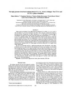
Figure 2: Schematic of an isotropic drop of radius R in an nematic ocean with radial director field. The interfacial unit normal m is directed outward from the nematic phase toward the origin.

Finally, we assume that Ψ = Ψ0 + Ψ1 + o()

(5.6)

with Ψ0 and Ψ1 given constants. Then, assuming that β2 is constant and neglecting inertia, (4.53) yields at zeroth and first order in ,  β3 V0 = −Ψ0 , (5.7) ◦ β3 V1 − β2 K 1 = (ψ0 + c)K1 + 2c divS0 n1 − Ψ1 . When the interfacial free energy is constant (i.e., c = 0) this relation takes the form ◦

−β2 K 1 + β3 V1 = ψ0 K1 − Ψ1 ,

(5.8)

which, for β2 = 0, is the classical curvature-flow equation (Gurtin 2000).

6

Radial symmetry. Isotropic drop in a nematic ocean

6.1

Kinematics

Consider an isotropic spherical drop of time-dependent radius R(t) surrounded by a nematic ocean with purely radial director field (Figure 2) n(x) =

x . |x|

(6.1)

Then, for |x| > R(t), G(x) =

1 (1 − n(x)⊗n(x)), |x|

˙ n(x) = 0,

¨ (x) = 0 n

and

(6.2)

Moreover, for the phase interface |x| = R(t), m(x, t)

=−

x , R(t)

˙ V (x, t) = −R(t),

K(x, t) = ◦

1 P(x, t), R(t)

m(x, t)

= 0,

◦

K(x, t) =

K(x, t) = −

2 , R(t)

˙ 2R(t) , 2 R (t)

      

(6.3)

20

P. Cermelli, E. Fried & M. E. Gurtin

with P = 1 − m ⊗ m. Also, on |x| = R(t), n(x) = −m(x, t),

G(x) =

1 P(x, t), R(t)

◦

˙ n(x) = n(x) = 0,

ξ = −1,

(6.4)

the last of which is a consequence of (6.4)1 .

6.2

Bulk results

We take the relative free-energy density of the nematic phase to have the standard form ˆ Ψ(n, grad n) = Ψ0 + 12 k1 (div n)2 + 12 k2 (n·curl n)2 + 12 k3 |n×curl n|2 + 12 (k2 + k4 )(|grad n|2 − (div n)2 ),

(6.5)

due to Oseen (1933), Z¨ ocher (1933), and Frank (1958). Here, following Ericksen (1966), we assume that the splay, twist, bend, and saddle-splay moduli k1 , k2 , k3 , and k4 obey k1 ≥ 0, k2 ≥ |k4 |, k3 ≥ 0, and 2k1 ≥ k2 +k4 . The term Ψ0 contains information about the free-energy density of the nematic phase relative to that of the isotropic phase. For fixed compositions and in the absence of external electromagnetic fields, we might expect Ψ0 to be negative at sufficiently low temperatures, positive at sufficiently high temperatures, and zero at some intermediate temperature. Similar remarks can be made about what to expect when the temperature is fixed, external fields are absent, but compositional fluctuations are allowed, etc. We refer to Ψ0 as the ambient free-energy difference. In view of (6.1) and (6.2), the free-energy density (6.5) specializes to κ ˆ Ψ(n(x), G(x)) = Ψ0 + , |x|2

(6.6)

κ = 2k1 − (k2 + k4 ) ≥ 0.

(6.7)

where we have introduced

Further, direct calculations show that ˆ ∂ Ψ(n(x), G(x)) κ = (1 − n(x)⊗n(x)), ∂G |x|

ˆ ∂ Ψ(n(x), G(x)) = 0. ∂n

(6.8)

Satisfaction of the bulk director momentum balance (2.15) on |x| > R(t) then follows from (6.2) and (6.8).

6.3

Interfacial results

By (6.4) and (6.8), a direct calculation shows that the interfacial director momentum balance (4.49) is satisfied on |x| = R(t). Further, by (6.3), (6.4), (6.6), and (6.8), the normal configurational force balance (4.53) simplifies to an ordinary differential equation κ 2σ β R˙ = Ψ0 − + 2 R R

(6.9)

for the position R of the phase interface. Here, we have introduced β = β3

and

¯ σ = ψ(−1).

(6.10)

Sharp-interface nematic-isotropic phase transitions without flow

21

Table 1: Equilibria for the ordinary differential equation (6.9).  Ψ0 < 0

R∗ =

1+

R∗ =

Ψ0 = 0

0 < Ψ0


σ2 κ

 R∗± =

R∗ =

κ 2σ

 1±

1−

σ κ = Ψ0 σ

κΨ0 σ2



σ Ψ0

(unstable)

R∗ → ∞

We assume the interfacial free-energy density is defined so that σ > 0.

(6.11)

The equilibria of the ordinary differential equation (6.9) are synopsized in Table 1 and the qualitative behavior of the solutions is depicted in Figure 3. Suppose that the isotropic drop initially occupies a sphere of radius R0 : R(0) = R0

(6.12)

To discuss the initial-value problem formed by (6.9) and (6.12), we consider separetly three regimes: Ψ0 < 0, Ψ0 = 0, and Ψ0 > 0. For Ψ0 < 0, (6.9) has a single equilibrium point   κ|Ψ0 | σ R∗ = . 1+ −1 σ2 |Ψ0 |

(6.13)

Thus, when the ambient energy of the nematic phase is less than that of the isotropic phase, the competition between nematic curvature elasticity and interfacial tension allows for the existence of a unique two-phase equilibrium state with an isotropic spherical drop in a nematic ocean. In a dynamical process, the radius R of the drop grows or shrinks from its initial value R0 until it reaches R∗ as given by (6.14) depending on whether 0 < R0 < R∗ or R∗ < R0 < ∞, respectively. For Ψ0 = 0, (6.9) still has a single stable equilibrium point R∗ =

κ , 2σ

(6.14)

and the qualitative behavior is the same as above. For Ψ0 > 0, we consider three subregimes: Ψ0


σ2 . κ

22

P. Cermelli, E. Fried & M. E. Gurtin R(t)

R(t)

R(t) R∗+ R∗−

R∗

t

t Ψ0 < 0

0 < Ψ0 < σ 2 /κ

t σ 2 /κ < Ψ0

Figure 3: Plots of the time-dependence of the radius of an isotropic drop in a radial nematic ocean, at different values of the ambient energy.

First, for Ψ0 < σ 2 /2κ, (6.9) has two equilibrium points    σ κΨ0 ± R∗ = 1 ± 1 − 2 , σ Ψ0

(6.15)

and R∗− is stable while R∗+ is unstable. In this regime the ambient energy of the nematic phase exceeds that of the isotropic phase, but the competition between nematic curvature elasticity and interfacial tension allows for the presence of stable isotropic spherical drops in a nematic ocean. For 0 < R0 < R∗+ , the radius R of the drop grows or shrinks from its initial value R0 until it reaches R∗− as given by (6.15), depending on whether 0 < R0 < R∗− or R∗− < R0 , respectively. For R∗+ < R0 < ∞, the region occupied by the isotropic phase grows at the expense of the nematic phase. Hence R∗+ is a critical radius for the phase transition: the drop must be sufficiently large to initiate a complete transformation to the isotropic phase. The fact that a nematic to isotropic transition that initiated with the nucleation of isotropic droplets requires that the drops coalesce to proceed further is consistent with observations. Next, for Ψ0 = σ 2 /κ, (6.9) has a single saddle equilibrium point σ κ R∗ = = . (6.16) Ψ0 σ Thus, in a dynamical process, the radius of the drop will always grow. Finally, for Ψ0 > σ 2 /κ, the isotropic phase grows without bound. Thus, when the ambient energy of the nematic phase exceeds that of the isotropic phase to the extent that it is greater than σ 2 /κ, the nematic phase is unstable.

Remarks (i) Reasonable orders of magnitude for the parameters κ and σ are (Stephen & Straley 1974) κ ∼ 10−7 erg/cm Thus, when the ambient energy difference vanishes, (6.14) gives R∗ ∼ 10−1 µm. Assuming that |Ψ0 |  σ 2 /κ and expanding (6.13) accordingly, we find that this value for R∗ ∼ σ/κ ∼ 10−1 µm as well. Further, for Ψ0  σ 2 /κ, (6.15) gives R∗− ∼ κ/σ ∼ 10−1 µm and R∗+ ∼ 2σ/Ψ0  R∗− . In each of these cases, the theory therefore yields drop radii on the order of 10−1 µm. Thus, since the characteristic dimension of a mesogen is 1 nm, R∗ as predicted by our theory is on the order of 102 molecular lengths. (ii) For Ψ0 > σ 2 /κ, i.e., when the isotropic to nematic transition is favored, different time scales characterize nucleation and growth. In fact, when R is sufficiently small, (6.9) should be well-approximated by κ β R˙ ∼ 2 , R

Sharp-interface nematic-isotropic phase transitions without flow

23

which implies that the, in the initial stage of growth immediately after nucleation, the drop radius evolves according to  R(t) ∼ 3 R0 + 3κt. Subsequently, there is a cross-over time where both terms −2σ/R and κ/R2 become important. √ Thereafter, the term Ψ0 − 2σ/R will dominate and the growth is diffusive (∼ t). Finally, once the radius is large enough, the constant term will dominate, and the growth is linear in time. Hence, the initial growth after nucleation is much faster than the steady growth of sufficiently large inclusions (cf. Figure 3). (iii) If we considered instead a radially-aligned nematic drop is an isotropic ocean, the foregoing results would be unchanged. (To achieve it all we would need to do is alter a few words and signs (m would be outward).) The analog of the foregoing result concerning a initial stage of rapid growth would then be consistent with the experiments of Ostner, Chan & Kahlweit (1973). (iv) Small isotropic spherical drops in a nematic radially oriented phase for Ψ0 ≤ 0, may be used to model the cores of hedgehog defects. Indeed, we may explicitly calculate ¯ > R∗ containing as the net (bulk plus surface) free-energy in a sphere of radius R isotropic drop to yield



 ¯ + 4π σR2 − 1 Ψ0 R∗ − κR∗ . ¯ 3 + κR 4π 13 Ψ0 R (6.17) ∗ 3 Of the two terms in (6.17) the first is the bulk energy of a hedgehog defect while the second is the correction due to the isotropic core; a straightforward calculation shows that, for Ψ0 ≤ 0 and R∗ given by (6.13) or (6.14), this correction is negative, so that the presence of the core decreases the free energy stored in the hedgehog.

Appendix Variation Lemma: (a) Let Φ = Φ(x, t) and Θ = Θ(x, t) be scalar bulk fields, and h = h(x, t) a bulk vector field. If    Φ dv + h·m∂R da ≤ ΘV∂R da, (6.18) R

∂R

∂R

for all migrating control volumes R, then Θ = 0. (b) Let u = u(x, t) and w = w(x, t) be superficial fields: if   u da ≤ wV∂A ds, A

(6.19)

(6.20)

∂A

for all migrating pillboxes A ⊂ S, then w = 0.

(6.21)

24

P. Cermelli, E. Fried & M. E. Gurtin

Proof: (a) Fix t = t0 , and choose arbitrarily a fixed region R0 . Letting r0 (ξ), ξ = (ξ1 , ξ2 ), be a parametrization of ∂R0 , define a migrating control volume R(t) so that r(ξ, t) = r0 (ξ) + c(t − t0 )φ(ξ)m∂R (ξ), is a parametrization of ∂R(t), where c is an arbitrary constant, φ is an arbitrary smooth function and m∂R is the outward unit normal to ∂R0 . Clearly, R(t0 ) = R0 and V∂R (ξ, t0 ) = cφ(ξ). Hence, letting    A := Φ dv + h·m∂R da, B := Θφ da, R0

∂R0

∂R0

(6.18) becomes A ≤ cB for any constant c. Now, if B = 0, choosing c < A/B when B  > 0 and c > A/B when B < 0, we obtain A < A, which is impossible. Hence, Θφ da = 0 for arbitrary φ and R0 , and this implies (6.19). ∂R0 (b) Now let r(ξ, t) be a parametrization of S(t), fix t0 and A0 ⊂ S(t0 ). If r(ξ 0 (s), t0 ) is a parametrization of the curve ∂A0 , define ξ(s, t) = ξ 0 (s) + c(t − t0 )φ(s)m(s), where m(s) is the 2-dimensional vector such that   ∂r (ξ 0 (s), t0 ) m(s) = m∂A (ξ 0 (s), t0 ), ∂ξ c is an arbitrary constant, and φ(s) and arbitrary real function. Then r(ξ(s, t), t) is the parametrization of the boundary ∂A(t) ⊂ S(t) of a migrating pillbox such that A(t0 ) = A0 . Moreover, at t = t0 , v∂A

= v + cφm∂A ,

V∂A = v · m∂A + cφ,

with v = ∂r/∂t. Hence, letting   α := u da − wv · m∂A ds, A0

∂A0

 β :=

wφ ds, ∂A0

(6.20) becomes α ≤ cβ for any c. Proceeding as in (a) we obtain (6.21).

Appendix P.C. was supported by the Italian M.I.U.R. project “Modelli matematici per la scienza dei materiali” during the completion of this work. E.F. and M.E.G. were supported by the National Science Foundation and the Department of Energy.

References Armitage, D. Price, F. P., 1978. Supercooling and nucleation in liquid crystals, Molecular Crystals and Liquid Crystals 44, 33–44. Anderson, D. R., Carlson, D. E., Fried, E., 1999. A continuum-mechanical theory for nematic elastomers, Journal of Elasticity 56, 33–58.

Sharp-interface nematic-isotropic phase transitions without flow

25

Cermelli, P., Fried, E., 2002. The evolution equation for a disclination in a nematic liquid crystal, Proceedings of the Royal Society of London A 458, 1–20. Cheong, A-G., Rey, A.D., 2002. Cahn–Hoffman capillarity vector thermodynamics for curved liquid crystal interfaces with application to fiber instabilities, Journal of Chemical Physics 117, 5062–5071. Derzhanski, A. I., Petrov, A. G., 1979. Flexoelectricity in nematic liquid crystals, Acta Physica Polonica A 55, 747–767. de Gennes, P. G., 1971. Short range order effects in the isotropic phase of nematics and cholesterics, Molecular Crystals and Liquid Crystals 12, 193–214. Ericksen, J. L., 1961. Conservation laws for liquid crystals, Transactions of the Society of Rheology 5, 23–34. Ericksen, J. L., 1966. Inequalities in liquid crystal theory, Physics of Fluids 9, 1205–1207. Eshelby, J. D., 1980. The force on a disclination in a liquid crystal, Philosphical Magazine A 42, 359–367. Frank, F. C., 1958. On the theory of liquid crystals, Discussions of the Faraday Society 25, 19–28. Gurtin, M. E., 1995. The nature of configurational forces, Archive for Rational Mechanics and Analysis 131, 67–100. Gurtin, M. E., 2000. Configurational Forces as Basic Concepts of Continuum Physics. New York: Springer. Gurtin, M. E., Jabbour, M. E., 2002. Interface evolution in three dimensions with curvaturedependent energy and surface diffusion: Interface-controlled evolution, phase transitions, epitaxial growth of elastic films, Archive for Rational Mechanics and Analyis 163, 171–208. Gurtin, M. E., Struthers, A., 1990. Multiphase thermomechanics with interfacial structure 3. Evolving phase boundaries in the presence of bulk deformation, Archive for Rational Mechanics and Analysis 112, 97–160. Gurtin, M. E., Struthers, A., Williams, W. O., 1989 A transport theorem for moving interfaces, Quarterly of Applied Mathematics 47, 773–777. Langer, J. S., 1980. Instabilities and pattern formation in cyrstal growth, Reviews of Modern Physics 52, 1–28. Leslie, F. M., 1968. Some constitutive equations for liquid crystals, Archive for Rational Mechanics and Analysis 28, 265–283. Maugin, G. A., Trimarco, C., 1995. On material and physical forces in liquid crystals, International Journal of Engineering Science 33, 1163–1678. Oseen, W. C., 1933. The theory of liquid crystals, Transactions of the Faraday Society 29, 883–899. Ostner, W., Chan, S.-K., Kahlweit, M., 1973. On the transformation of a liquid crystal (pAzoxydianisole) from its isotropic to its nematic state, Berichte der Bunsen-Gesellschaft f¨ ur physicalische Chemie 77, 1122–1126. Oswald, P., Bechhoefer, J., Libchaber, A., 1987. Instabilities of a moving nematic-isotropic interface, Physical Review Letters 58, 2318–2321. Poniewierski, A., 2000. Shape of the nematic-isotropic interface in conditions of partial wetting. Liquid Crystals 27, 1369–1380. Rapini, A., Papoular, M., 1969. Distorsion d’une lamelle n´ematique sous champ magn´etique. Conditions d’ancrage aux parois, Journal de Physique (Paris) Colloque C4 30, 54–56. Rey, A. D., 2000a. Young–Laplace equation for liquid crystal interfaces. Journal of Chemical Physics 113 (2000), 10820–10822. Rey, A. D., 2000b. Viscoelastic theory for nematic interfaces. Physical Review E 61, 1540–1549. Rey, A. D., 2000c. Theory of interfacial dynamics of nematic polymers. Rheologica Acta 39, 13–19. Rey, A. D., 2001. Mechanical theory for nematic thin films. Langmuir 17, 1922–1927. Stephen, M. J., Straley, J. P., 1974. Physics of liquid crystals, Reviews of Modern Physics 46, 617–704. Z¨ ocher, H., 1933. The effect of a magnetic field on the nematic state, Transactions of the Faraday Society 29, 945–957.

List of Recent TAM Reports No.

Authors

955 Fried, E.

Title

An elementary molecular-statistical basis for the Mooney and Rivlin–Saunders theories of rubber-elasticity—Journal of the Mechanics and Physics of Solids 50, 571–582 (2002) 956 Phillips, W. R. C. On an instability to Langmuir circulations and the role of Prandtl and Richardson numbers—Journal of Fluid Mechanics 442, 335–358 (2001) 957 Chaïeb, S., and J. Sutin Growth of myelin figures made of water soluble surfactant— Proceedings of the 1st Annual International IEEE–EMBS Conference on Microtechnologies in Medicine and Biology (October 2000, Lyon, France), 345–348 958 Christensen, K. T., and Statistical evidence of hairpin vortex packets in wall turbulence— R. J. Adrian Journal of Fluid Mechanics 431, 433–443 (2001) 959 Kuznetsov, I. R., and Modeling the thermal expansion boundary layer during the D. S. Stewart combustion of energetic materials—Combustion and Flame, in press (2001) 960 Zhang, S., K. J. Hsia, Potential flow model of cavitation-induced interfacial fracture in a and A. J. Pearlstein confined ductile layer—Journal of the Mechanics and Physics of Solids, 50, 549–569 (2002) 961 Sharp, K. V., Liquid flows in microchannels—Chapter 6 of CRC Handbook of R. J. Adrian, MEMS (M. Gad-el-Hak, ed.) (2001) J. G. Santiago, and J. I. Molho 962 Harris, J. G. Rayleigh wave propagation in curved waveguides—Wave Motion 36, 425–441 (2002) 963 Dong, F., A. T. Hsui, A stability analysis and some numerical computations for thermal and D. N. Riahi convection with a variable buoyancy factor—Journal of Theoretical and Applied Mechanics 2, 19–46 (2002) 964 Phillips, W. R. C. Langmuir circulations beneath growing or decaying surface waves—Journal of Fluid Mechanics (submitted) 965 Bdzil, J. B., Program burn algorithms based on detonation shock dynamics— D. S. Stewart, and Journal of Computational Physics (submitted) T. L. Jackson 966 Bagchi, P., and Linearly varying ambient flow past a sphere at finite Reynolds S. Balachandar number: Part 2—Equation of motion—Journal of Fluid Mechanics 481, 105–148 (2003) (with change in title) 967 Cermelli, P., and The evolution equation for a disclination in a nematic fluid— E. Fried Proceedings of the Royal Society A 458, 1–20 (2002) 968 Riahi, D. N. Effects of rotation on convection in a porous layer during alloy solidification—Chapter 12 in Transport Phenomena in Porous Media (D. B. Ingham and I. Pop, eds.), 316–340 (2002) 969 Damljanovic, V., and Elastic waves in cylindrical waveguides of arbitrary cross section— R. L. Weaver Journal of Sound and Vibration (submitted) 970 Gioia, G., and Two-phase densification of cohesive granular aggregates—Physical A. M. Cuitiño Review Letters 88, 204302 (2002) (in extended form and with added co-authors S. Zheng and T. Uribe) 971 Subramanian, S. J., and Calculation of a constitutive potential for isostatic powder P. Sofronis compaction—International Journal of Mechanical Sciences (submitted) 972 Sofronis, P., and Atomistic scale experimental observations and micromechanical/ I. M. Robertson continuum models for the effect of hydrogen on the mechanical behavior of metals—Philosophical Magazine (submitted) 973 Pushkin, D. O., and Self-similarity theory of stationary coagulation—Physics of Fluids 14, H. Aref 694–703 (2002) 974 Lian, L., and Stress effects in ferroelectric thin films—Journal of the Mechanics and N. R. Sottos Physics of Solids (submitted) 975 Fried, E., and Prediction of disclinations in nematic elastomers—Proceedings of the R. E. Todres National Academy of Sciences 98, 14773–14777 (2001)

Date Sept. 2000 Sept. 2000 Oct. 2000

Oct. 2000 Oct. 2000 Nov. 2000 Nov. 2000

Jan. 2001 Jan. 2001 Jan. 2001 Jan. 2001 Feb. 2001 Apr. 2001 Apr. 2001 May 2001 May 2001 June 2001 June 2001 July 2001 Aug. 2001 Aug. 2001

List of Recent TAM Reports (cont’d) No.

Authors

976 Fried, E., and V. A. Korchagin 977 Riahi, D. N.

Title

Striping of nematic elastomers—International Journal of Solids and Structures 39, 3451–3467 (2002) On nonlinear convection in mushy layers: Part I. Oscillatory modes of convection—Journal of Fluid Mechanics 467, 331–359 (2002) 978 Sofronis, P., Recent advances in the study of hydrogen embrittlement at the I. M. Robertson, University of Illinois—Invited paper, Hydrogen–Corrosion Y. Liang, D. F. Teter, Deformation Interactions (Sept. 16–21, 2001, Jackson Lake Lodge, and N. Aravas Wyo.) 979 Fried, E., M. E. Gurtin, A void-based description of compaction and segregation in flowing and K. Hutter granular materials—Continuum Mechanics and Thermodynamics, in press (2003) 980 Adrian, R. J., Spanwise growth of vortex structure in wall turbulence—Korean S. Balachandar, and Society of Mechanical Engineers International Journal 15, 1741–1749 Z.-C. Liu (2001) 981 Adrian, R. J. Information and the study of turbulence and complex flow— Japanese Society of Mechanical Engineers Journal B, in press (2002) 982 Adrian, R. J., and Observation of vortex packets in direct numerical simulation of Z.-C. Liu fully turbulent channel flow—Journal of Visualization, in press (2002) 983 Fried, E., and Disclinated states in nematic elastomers—Journal of the Mechanics R. E. Todres and Physics of Solids 50, 2691–2716 (2002) 984 Stewart, D. S. Towards the miniaturization of explosive technology—Proceedings of the 23rd International Conference on Shock Waves (2001) 985 Kasimov, A. R., and Spinning instability of gaseous detonations—Journal of Fluid Stewart, D. S. Mechanics (submitted) 986 Brown, E. N., Fracture testing of a self-healing polymer composite—Experimental N. R. Sottos, and Mechanics (submitted) S. R. White 987 Phillips, W. R. C. Langmuir circulations—Surface Waves (J. C. R. Hunt and S. Sajjadi, eds.), in press (2002) 988 Gioia, G., and Scaling and similarity in rough channel flows—Physical Review F. A. Bombardelli Letters 88, 014501 (2002) 989 Riahi, D. N. On stationary and oscillatory modes of flow instabilities in a rotating porous layer during alloy solidification—Journal of Porous Media 6, 1–11 (2003) 990 Okhuysen, B. S., and Effect of Coriolis force on instabilities of liquid and mushy regions D. N. Riahi during alloy solidification—Physics of Fluids (submitted) 991 Christensen, K. T., and Measurement of instantaneous Eulerian acceleration fields by R. J. Adrian particle-image accelerometry: Method and accuracy—Experimental Fluids (submitted) 992 Liu, M., and K. J. Hsia Interfacial cracks between piezoelectric and elastic materials under in-plane electric loading—Journal of the Mechanics and Physics of Solids 51, 921–944 (2003) 993 Panat, R. P., S. Zhang, Bond coat surface rumpling in thermal barrier coatings—Acta and K. J. Hsia Materialia 51, 239–249 (2003) 994 Aref, H. A transformation of the point vortex equations—Physics of Fluids 14, 2395–2401 (2002) 995 Saif, M. T. A, S. Zhang, Effect of native Al2O3 on the elastic response of nanoscale aluminum A. Haque, and films—Acta Materialia 50, 2779–2786 (2002) K. J. Hsia 996 Fried, E., and A nonequilibrium theory of epitaxial growth that accounts for M. E. Gurtin surface stress and surface diffusion—Journal of the Mechanics and Physics of Solids 51, 487–517 (2003) 997 Aref, H. The development of chaotic advection—Physics of Fluids 14, 1315– 1325 (2002); see also Virtual Journal of Nanoscale Science and Technology, 11 March 2002

Date Aug. 2001 Sept. 2001 Sept. 2001

Sept. 2001 Sept. 2001 Oct. 2001 Oct. 2001 Oct. 2001 Oct. 2001 Oct. 2001 Nov. 2001 Nov. 2001 Nov. 2001 Nov. 2001 Dec. 2001 Dec. 2001 Dec. 2001 Jan. 2002 Jan. 2002 Jan. 2002 Jan. 2002 Jan. 2002

List of Recent TAM Reports (cont’d) No.

Authors

Title

998 Christensen, K. T., and The velocity and acceleration signatures of small-scale vortices in R. J. Adrian turbulent channel flow—Journal of Turbulence, in press (2002) 999 Riahi, D. N. Flow instabilities in a horizontal dendrite layer rotating about an inclined axis—Journal of Porous Media, in press (2003) 1000 Kessler, M. R., and Cure kinetics of ring-opening metathesis polymerization of S. R. White dicyclopentadiene—Journal of Polymer Science A 40, 2373–2383 (2002) 1001 Dolbow, J. E., E. Fried, Point defects in nematic gels: The case for hedgehogs—Proceedings and A. Q. Shen of the National Academy of Sciences (submitted) 1002 Riahi, D. N. Nonlinear steady convection in rotating mushy layers—Journal of Fluid Mechanics 485, 279–306 (2003) 1003 Carlson, D. E., E. Fried, The totality of soft-states in a neo-classical nematic elastomer— and S. Sellers Journal of Elasticity 69, 169–180 (2003) with revised title 1004 Fried, E., and Normal-stress differences and the detection of disclinations in R. E. Todres nematic elastomers—Journal of Polymer Science B: Polymer Physics 40, 2098–2106 (2002) 1005 Fried, E., and B. C. Roy Gravity-induced segregation of cohesionless granular mixtures— Lecture Notes in Mechanics, in press (2002) 1006 Tomkins, C. D., and Spanwise structure and scale growth in turbulent boundary R. J. Adrian layers—Journal of Fluid Mechanics (submitted) 1007 Riahi, D. N. On nonlinear convection in mushy layers: Part 2. Mixed oscillatory and stationary modes of convection—Journal of Fluid Mechanics (submitted) 1008 Aref, H., P. K. Newton, Vortex crystals—Advances in Applied Mathematics 39, in press (2002) M. A. Stremler, T. Tokieda, and D. L. Vainchtein 1009 Bagchi, P., and Effect of turbulence on the drag and lift of a particle—Physics of S. Balachandar Fluids, in press (2003) 1010 Zhang, S., R. Panat, Influence of surface morphology on the adhesive strength of and K. J. Hsia aluminum/epoxy interfaces—Journal of Adhesion Science and Technology 17, 1685–1711 (2003) 1011 Carlson, D. E., E. Fried, On internal constraints in continuum mechanics—Journal of and D. A. Tortorelli Elasticity 70, 101–109 (2003) 1012 Boyland, P. L., Topological fluid mechanics of point vortex motions—Physica D M. A. Stremler, and 175, 69–95 (2002) H. Aref 1013 Bhattacharjee, P., and Computational studies of the effect of rotation on convection D. N. Riahi during protein crystallization—Journal of Crystal Growth (submitted) 1014 Brown, E. N., In situ poly(urea-formaldehyde) microencapsulation of M. R. Kessler, dicyclopentadiene—Journal of Microencapsulation (submitted) N. R. Sottos, and S. R. White 1015 Brown, E. N., Microcapsule induced toughening in a self-healing polymer S. R. White, and composite—Journal of Materials Science (submitted) N. R. Sottos 1016 Kuznetsov, I. R., and Burning rate of energetic materials with thermal expansion— D. S. Stewart Combustion and Flame (submitted) 1017 Dolbow, J., E. Fried, Chemically induced swelling of hydrogels—Journal of the Mechanics and H. Ji and Physics of Solids, in press (2003) 1018 Costello, G. A. Mechanics of wire rope—Mordica Lecture, Interwire 2003, Wire Association International, Atlanta, Georgia, May 12, 2003 1019 Wang, J., N. R. Sottos, Thin film adhesion measurement by laser induced stress waves— and R. L. Weaver Journal of the Mechanics and Physics of Solids (submitted) 1020 Bhattacharjee, P., and Effect of rotation on surface tension driven flow during protein D. N. Riahi crystallization—Microgravity Science and Technology, in press (2003)

Date Jan. 2002 Feb. 2002 Feb. 2002 Feb. 2002 Mar. 2002 Mar. 2002 June 2002 July 2002 Aug. 2002 Sept. 2002 Oct. 2002

Oct. 2002 Oct. 2002 Oct. 2002 Oct. 2002 Feb. 2003 Feb. 2003

Feb. 2003 Mar. 2003 Mar. 2003 Mar. 2003 Apr. 2003 Apr. 2003

List of Recent TAM Reports (cont’d) No.

Authors

Title

Date

1021 Fried, E.

Apr. 2003

1022

May 2003

1023 1024 1025 1026 1027 1028 1029 1030 1031

1032

1033 1034 1035 1036 1037 1038 1039

The configurational and standard force balances are not always statements of a single law—Proceedings of the Royal Society (submitted) Panat, R. P., and Experimental investigation of the bond coat rumpling instability K. J. Hsia under isothermal and cyclic thermal histories in thermal barrier systems—Proceedings of the Royal Society of London A, in press (2003) Fried, E., and A unified treatment of evolving interfaces accounting for small M. E. Gurtin deformations and atomic transport: grain-boundaries, phase transitions, epitaxy—Advances in Applied Mechanics, in press (2003) Dong, F., D. N. Riahi, On similarity waves in compacting media—Horizons in Physics, in and A. T. Hsui press (2003) Liu, M., and K. J. Hsia Locking of electric field induced non-180° domain switching and phase transition in ferroelectric materials upon cyclic electric fatigue—Applied Physics Letters, in press (2003) Liu, M., K. J. Hsia, and In situ X-ray diffraction study of electric field induced domain M. Sardela Jr. switching and phase transition in PZT-5H—Journal of the American Ceramics Society (submitted) Riahi, D. N. On flow of binary alloys during crystal growth—Recent Research Development in Crystal Growth, in press (2003) Riahi, D. N. On fluid dynamics during crystallization—Recent Research Development in Fluid Dynamics, in press (2003) Fried, E., V. Korchagin, Biaxial disclinated states in nematic elastomers—Journal of Chemical and R. E. Todres Physics 119, 13170–13179 (2003) Sharp, K. V., and Transition from laminar to turbulent flow in liquid filled R. J. Adrian microtubes—Physics of Fluids (submitted) Yoon, H. S., D. F. Hill, Reynolds number scaling of flow in a Rushton turbine stirred tank: S. Balachandar, Part I—Mean flow, circular jet and tip vortex scaling—Chemical R. J. Adrian, and Engineering Science (submitted) M. Y. Ha Raju, R., Reynolds number scaling of flow in a Rushton turbine stirred tank: S. Balachandar, Part II—Eigen-decomposition of fluctuation—Chemical Engineering D. F. Hill, and Science (submitted) R. J. Adrian Hill, K. M., G. Gioia, Structure and kinematics in dense free-surface granular flow— and V. V. Tota Physical Review Letters, in press (2003) Fried, E., and S. Sellers Free-energy density functions for nematic elastomers—Journal of the Mechanics and Physics of Solids, in press (2003) Kasimov, A. R., and On the dynamics of self-sustained one-dimensional detonations: D. S. Stewart A numerical study in the shock-attached frame—Physics of Fluids (submitted) Fried, E., and B. C. Roy Disclinations in a homogeneously deformed nematic elastomer— Nature Materials (submitted) Fried, E., and The unifying nature of the configurational force balance—Mechanics M. E. Gurtin of Material Forces (P. Steinmann and G. A. Maugin, eds.), in press (2003) Panat, R., K. J. Hsia, Rumpling instability in thermal barrier systems under isothermal and J. W. Oldham conditions in vacuum—Philosophical Magazine (submitted) Cermelli, P., E. Fried, Sharp-interface nematic–isotropic phase transitions without flow— and M. E. Gurtin Archive for Rational Mechanics and Analysis (submitted)

May 2003 May 2003 May 2003 May 2003 May 2003 July 2003 July 2003 July 2003 Aug. 2003

Aug. 2003

Aug. 2003 Sept. 2003 Nov. 2003 Nov. 2003 Dec. 2003 Dec. 2003 Dec. 2003