Short-range wireless sensor networks for high ... - Semantic Scholar

Short-range wireless sensor networks for high density seismic monitoring 1

S. Savazzi1,2 , L. Goratti3 , U. Spagnolini2 , M. Latva-aho3 Wireless Systems for Geophysics (WiSyGEO), Milano (Italy); 2 D.E.I., Politecnico di Milano, Italy 3 Centre for Wireless Communications (CWC), University of Oulu, Finland e-mail: (savazzi, spagnoli)@elet.polimi.it, (matti.latvaaho,goratti)@ee.oulu.fi

Abstract— Acquisition systems for sub-surface diagnostic (for small earthquake monitoring) and exploration (for new oil and gas reservior) require a large number of sensors (geophones or accelerometers) to be deployed in outdoor over large areas to measure backscattered wave fields. A storage/processing unit (sink node) collects the measurements from all the geophones to obtain an image of the sub-surface for real-time analysis of seismic activity. In-depth imaging quality depends on the number of sensors deployed and on the position accuracy for each sensing device. Current connectivity is cable based and in some cases requires hundreds of kilometers of cabling while synchronous acquisition is obtained thorugh GPS causing large power consumption and degradation in accuracy. Replacing cables with wireless connectivity to create a wireless geophone network (WGN) is now becoming attractive to improve the monitoring quality and enable synchronous monitoring (and self-localization) with minimal use of GPS. This paper serves as a tutorial to introduce the basic principles of seismic monitoring systems from a wireless communication perspective. Specifications for the network architecture and the MAC layer are proposed to replace the actual cabled systems.

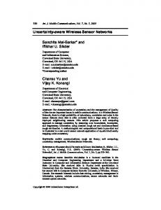
Active seismic monitoring Source

Receivers

Gas/Oil/Water

Gas/Oil/Water

Shooting phase

Data Delivery phase Delivery

Shot

time

time

Passive seismic monitoring Receivers

Dip-slip fau lt

Dip -slip fault

Index Terms— Seismic monitoring, Ultra-Wide Band, Mesh networking, Cooperative Localization Fig. 1. Example of seismic monitoring settings: active and passive monitoring

I. I NTRODUCTION Wireless Sensor Networks (WSNs) represent well-known paradigm that collects a set of emerging technologies that will have profound effects across a range of industrial, scientific and governmental applications [1]. Recent developments in wireless technologies and semiconductor fabrication of battery-powered miniature sensors are making WSNs more cost-effective for a growing number of pervasive applications. New radio technologies such as Ultra-Wide Band (UWB) and Multi-Band OFDM (MB-OFDM) [2] are expected to provide tiny and low power sensors with the capability of supporting raw data rates within very short range distances. Although a wide number of applications have been proposed for WSN [1], their market penetration and volumes do not currently seem to offer the expected opportunity to fully explore the potential of the latest cutting-edge technologies. Wireless community could therefore look at the new cable replacing applications that can guarantee WSN systems to move towards larger business volumes. Acquisition systems for seismic monitoring can be classified into active and passive systems. Passive monitoring systems This work is partially supported by Ministero dell’Istruzione dell’Universita’ e della Ricerca MIUR-FIRB Integrated System for Emergency (InSyEme) project under the grant RBIP063BPH.

(PSM) are designed to acquire and analyzie, in real-time, the acoustic signals to identify small earthquakes (microseism) and to perform sub-surface diagnostic. Active monitoring systems (ASM) collect the seismic data from all the sensors to acquire a picture of the sub-surface to identify new oil and gas reservoir. The envisioned production peak of current oil and gas reservoirs is pushing the oil companies to increase the investments in seismic exploration of new oil reservoirs and in new technologies to improve the quality of depth imaging [3]. Seismic monitoring systems require a large number of sensors (geophones or accelerometers) to be deployed over wide areas to form large arrays that measure (and digitalize) back-scattered wave fields. A storage/processing unit (sink node) collects all the measurements from all the geophones. Typical cable-based surveys require hundreds of kilometers of cabling, moreover they impose stringent constraints on the survey design as the cables impact on the grid size and the particular acquisition geometry. Replacing cables with wireless connectivity is now becoming attractive to reduce the logistic and weight costs and improve the monitoring quality. The wireless geophone network (WGN) [4] is made up of battery-powered geophones that are self-localizing and monitoring synchronously without the need of land-surveyors.

2

Moving from wired to wireless has several advantages: first of all, WGN can reduce the high cabling, installation and maintenance cost (active seismic monitoring requires up to 10.000 man-hours/sqkm) of traditional wired data-acquisition systems. Furthermore, tiny wireless devices are easily deployable to make the acquisition structure more flexible and dense (say 1000 − 2000 devices/sqkm) with improved monitoring quality (sub-surface imaging). Technical limitations of well-consolidated WiFi/Bluetooth technologies (in terms of data-rate efficiency, interference, battery-use, propagation-loss, etc. . . ) force the current proposals for WGN architectures to choose a mix of wireless and cables [4]. Recent advances in WSN technology have led the wireless community to become now mature to meet the rigid constraints imposed by seismic acquisition systems. The goal of this paper is twofold: at first, it is provided a tutorial to introduce the basic principles of seismic acquisition systems by underlying the basic features and requirements from a wireless communication perspective. In particular, we focus on the more stringent network requirements that are mandatory for seismic exploration (Active Seismic Monitoring). Second, the specifications for the MAC/PHY layer are developed to enable self-localization WGN, synchronous monitoring and real-time data delivery. The paper is organized as follows: after a brief tutorial on land seismic acquisition system (Sect.II), in Sect.III it is proposed a mixed architecture that can fit with the constraints of WGN. Once defined the architecture, the main PHY and MAC layer specifics are outlined in Sect.III-A. II. L AND SEISMIC ACQUISITION SYSTEMS In this section we provide an outline of the basic principles of seismic prospecting (the reader might refer to the wide literature for more in-depth discussion, see e.g., [3]). On the surface, one (or more) energy source(s) (e.g., dynamite or a controlled-source as a vibrated plate) referred to as source point generates elastic waves that propagate over the subsurface. These elastic waves are reflected and refracted by any media discontinuity with different elastic properties. Sensors (geophones or MEMS based accelerometers) are activating a number of seismic channels to measure the back-scattered wavefield that convey reflected elastic energy. Digital signals are sent to a storage/processing unit (sink node). Acquisition system consists of two distinct phases that are repeated periodically: 1) the shooting phase where one (or more) source(s) placed in a predefined position(s) is generating the elastic wave 2) the data delivery phase where the digital seismic data is measured and forwarded by the geophones to the storage unit. As shown in figure 1, shooting and data delivery are repeated periodically by moving the impulse source(s) over a grid of (typically) 20 ÷ 30m of spacing (shot interval, see 2D network geometry in figure 2). The storage/processing unit estimates the elastic discontinuities of the sub-surface by combining the data received from all the geophones. The goal is to create a picture of the sub-surface that might be indicative of new oil/gas reservoir. The quality of depth imaging scales

with the number of geophones (e.g., the receiver density) and on the field extension. In what follows we focus on the data delivery phase by focusing on the basic network requirements (in terms of sensor density and throughput), details on network topology are also summarized in figure 2. The reader might refer to [3]-[4] for further details on the seismic exploration. Network geometry and size. High density land seismic acquisition systems will provide up to N = 30.000 − 50.000 seismic channels (sensors simultaneously active) [3] with typical densities of 2000 sensors/sqkm. The field extension for one survey can be extremely large (up to 30 km2 , although larger field size is expected in the future). Sensors are deployed on the surface to form a number of receiver lines or arrays with an application-specific deployment as outlined in figure 2. A receiver line might consist of up 2000 geophones: each line is made of multiple micro-lines with sensors ideally placed over rectangular (or rhombic) lattice with horizontal (in-line) and vertical (cross-line) spacing of ∆x = 10 ÷ 30m and ∆y = 5 ÷ 10m, respectively. Natural and man-made obstructions make the network deployment far from being regular in practice. A similar topology is designed for the sources deployment. Network throughput. Sensor activity consists in sampling back-scattered wave-field with minimum sampling time Ts = 0.5ms, samples are digitalized using b = 24 bits resulting in an overall per-node data rate of R = b/Ts ' 50kbps. Typical three component (3C) seismic accelerometers combines the data received from (up to) three different channels so that the overall data rate can be three times larger as R ' 150kbps. Since one survey might require up to 30.000 sensors, the aggregated throughput for one survey, where all sensors are transferring real-time all data to storage unit, can be as high as N × R ' 4.5Gbps1 . Energy Consumption and Delay constraints. Advanced acquisition systems2 requires sensors to be designed for working (recording and transmitting) continuously for days (3 ÷ 7 days up to one month) so that seismic instrumentation might be left unattended for a long period. Land surveyors that are monitoring the status of the recording process must be capable of controlling the quality of the received data in real time. Synchronous acquisition and remote control. The storage unit provides with the necessary functions of i) starting and ending acquisition; ii) uplink/downlink monitoring of each sensor; iii) synchronizing the acquisition with maximum timing skew that is a fraction of the sampling time Ts , say below 10μs. Localization. Seismic acquisitions require land surveyors to collect the effective position and elevation information for each receiver. A complication in measuring the true receiver position is that natural and man-made obstructions can make the actual acquisition deployment to be largely different from nominal geometry. Accurate positioning after geophone 1 Typical aggregated throughput can vary depending on the type sensor (number of components) and field extension. Aggregated throughput of one receiver line can be in the order of 300Mbps 2 For vibroseis land acquisition cascaded sweep methos [5] eliminate the reset time in between two shootings, allowing for contiuous data recording from the sensors.

3

Shot line interval: 200-300m

R y = 20 − 40m

Storage Unit

Receiver line Shot point

Δ x= 10 − 30m Receiver Group interval

Δ y = 5 − 10 m

Micro-line

Seismic acquisition: 2D network topology.

Wireless Sensor Gateway (WSG)

WiFi

Storage Unit

s 5-60Mbp

UW (M B BOF DM )

50-150kbps Cluster

Sub-Network (SN)

300-400 nodes

Fig. 2.

Receiver line spacing: 200-300m

R=150kbps

Shot line

Shot line

30m

Receiver line

Wireless Sensor Cluster-head (WSC) Wireless Sensor (WS)

Fig. 3.

Wireless Geophone Network system architecture.

deployment (with error below 1m) is mandatory to avoid degradation of depth imaging quality. III. W IRELESS G EOPHONE N ETWORK : M EDIUM ACCESS C ONTROL AND ARCHITECTURE A wireless geophone network must support multiple acquisition settings and a wide set of applications [6]. Compared to cabled systems, it is expected to provide better spatial sampling and be independent on the type of sensor devices and on the number of supported seismic channels. Given the large field extension that the WGN is required to monitor, an heterogeneous network that exploits the advantages of long and short range radio technologies seems to appear a very attractive solution. Short-range radio technology can fulfil the network requirements within a limited region of space while long-range radio can handle the interconnection with the remote storage unit (remote sink). Furthermore, the outdoor environment under consideration significantly differs from the typical indoor propagation in terms of attenuation and multipath. It might be therefore assumed that even a short range technology might cover a longer distance compared to those measured in indoor environments. Figure 3 shows the hierarchical Wireless Geophone Network architecture supporting short and long range communications. The wide scene of figure 3 is broken into sub-network (SNs) managed by a wireless sensor Gateway node (WSG) serving

as coordinator (as local sink) and connecting to the storage unit (CSU). The WSG is expected to manage two radio technologies: the long-range technology is used to connect to the CSU while the short-range radio is used to cover the SN. Data forwarding within each SN is managed by a number of wireless sensor cluster-head (WSC) devices. WSC devices form a mesh network that collects data from a number of reduced function wireless sensors (WSs). A WSC might be a sensor itself or just a relay node that collects and route data from the WSs towards the WSC. The type of SN under consideration requires tight time synchronization and mandatory self-localization. Given all the constraints, UWB technology might become the natural choice at the physical layer. Within each SN it is envisaged that the physical layer technology is MB-OFDM. The use of MB-OFDM can enable a synchronization acquisition without deploying a fully GPS based network, with remarkable saving in terms of costs and battery usage. Furthermore the SN network is expected to enable considerable spatial reuse, thanks to the radio characteristics of the MB-OFDM. Finally, MB-OFDM technology can achieve good coexistence with other radio technologies (e.g., WiFi or WiMAX), without paying meaningful cross-interferences. To limit the interference caused by neighboring SNs that are simultaneous operating, devices belonging to different SNs are transmitting over different sub-bands using a pre-defined Fixed Frequency Interleaved channel (FFI) to resemble a cellular structure (see Fig. 3)3 . Summarizing, the heterogeneous mesh network that it is proposed so far exploits four different types of devices: • the wireless sensor units (WS) that deliver digital data to/from sensor(s), • the wireless sensor cluster-head (WSC) that locally collects data from a group of WSs, forwarding the data to the WSG, • the wireless sensor gateway (WSG) that collects the aggregated data from different WSCs forwarding them to the CSU, • the control and storage unit (CSU) that stores data from neighbor WSGs. A. ECMA-368 based cluster-mesh topology for WGN In what follows we focused our attention to the MAC specifics to be designed for MB-OFDM devices within one SN. The MAC protocol described is used to achieve network synchronization and to enable data exchange. The superframe is shown in Fig. 4 with the basic structure taken from the ECMA-368 standard [9]. Given the high node density and the geographically large scenario, it is proposed a hybrid solution for the network architecture. In particular we combine the benefits of both distributed and centralized approaches. As very well known, random access schemes (RAs) are sensitive to collisions and they present the typical cusp behavior as the offered traffic increases. On the other hand, RAs are more scalable with respect to static channel allocation schemes as time division multiple access (TDMA), which however better suit certain types of real-time applications. More flexibility 3 The

WSG MB-OFDM radio is initialized to operate on a specific sub-band.

4

WSG Beacon Slot

Beacon Period (BP)

Guaranteed Time Slots (GTS)

Contention access period slotted CSMA (CAP)

Wireless Sensor Gateway (WSG)

A

C

Super Frame B

D

E F

I L M

G H

Signalling Slots

Fig. 4.

DEV I

DEV M

DEV C

DEV D

Localization Beacons

DEV B

WSG

Localization frame

DEV A

WSC → WS

Newcomer device DEV E,F,G,H,L

signalling slots

Uplink TS Downlink WS → WSC TS

Wireless Sensor Cluster-head (WSC) Wireless Sensor (WS) reduced function

Sub-Network (SN)

HOBS

Newcomer devices can adaptively choose to become either cluster-heads (WSC) or reduced-function wireless sensors (WS) at time of network formation. Decision is made locally by each device based on: 1) GPS status (WSC must be equipped with GPS) 2) BP occupacy indicator

WGN Medium Access Control: superframe structure. Fig. 5.

is offered by a MAC that is able to combine both channel accesses [9]. As described in the previous section each SN is sub-divided into clusters managed by a WSC device. Inside each cluster the WS devices are recording the seismic data. Data is collected by each WSC and it is delivered to the WSG (the coordinator of the SN) by mesh mode. This cluster-mesh hierarchical structure and the superframe of Fig. 3 are the core of the proposed network. The WSG and the WSC devices are GPS equipped, whereas the WS devices not. Each cluster forms a typical star topology, where non-GPS sensor devices connect only to the WSC. The WSC periodically issues a beacon frame that maintain local synchronization inside the cluster, refreshing also general network information. Device inside clusters communicate using RA. This structure offers the advantage of scaling down the network size, hence relieving the collision problem. The network architecture inside a cluster resembles the classical IEEE std 802.15.4 star topology [10]. The achievement of tight synchronization is a mandatory feature of this type of networks. Therefore, the synchronization amongst the WSC devices and the Gateway is achieved by using the distributed beaconing concept of ECMA-368 [9]. In this case, a basic difference is that only the WSG and the WSC devices (GPS equipped) have the right to access the beacon period (BP), broadcasting a unique beacon frame in a collision-free beacon slot. In fact, in this case the WSG occupies by default the first beacon slot after the signalling slots, whereas WSC devices compete making first access on the two signalling slots. The device that wins the contention is elected to occupy the first beacon slot after the highest occupied beacon slot (HOBS). Two main advantages of this structure stand out: i) easy-to-spread synchronization and acquisition timing (through application dependent Information Elements, see Fig.5) amongst the different WSC devices; ii) again scale down the number of devices that access the BP. The former is given by the fact that the WSG issues a unique reference time, referred to as the beacon period start time (BPST) through its beacon frame; the latter avoids to saturate the BP, that is of course of finite size. With this mechanism we also keep the length of the beacon period as short as possible, hence limiting the energy expenditure during the set up phase of the network. After each cluster has recorded the data from a certain

Acquisition timing propagation and cluster formation.

experiment, the different WSCs have to report them to the WSG (fall-back phase). The fall-back procedure is handled by WSC devices that are interconnecting in mesh mode: given that only a fraction of the WSCs are covered by the WSG, it is needed a way of routing data towards the WSG-sink node. The WSC devices use the so called distributed reservation protocol (DRP) defined in [9] to route data between themselves by exploiting the middle part of the superframe. Again using the terminology of the IEEE std. 802.15.4, we refer to this portion of the superframe as the guaranteed time slots (GTS) [10]. Differently with respect to the standard the allocation of the GTS is done in a completely distributed fashion. This proposed structure offers the advantage of scaling down the network size, hence relieving the collision problem and limiting the energy expenditure during the set-up phase of the network. B. Cooperative Localization Protocol The main objective of the proposed cooperative localization protocol is to provide a method to exploit the high accuracy/precision ranging measurements from UWB signals (using the measurements from both GPS equipped devices and reduced-function devices without GPS) and to eliminate the turnaround latency and clock off-set issues (enabling two-way message exchange for ranging estimations). Consider N UWB devices belonging to the same beacon group with locations θ1 , . . . , θ N , each defined by a pair of spatial coordinates θk = [xk yk ] ∈ R2 , k = 1, . . . , N . We assume that the first Nu nodes are WS with unknown positions θ = [θ1 · · · θNu ]T = [xT yT ]T , with x = [x1 · · · xNu ]T and y = [y1 · · · yNu ]T , while the remaining Nr = N − Nu are cluster-heads (WSC) located in known positions θr = [θNu +1 · · · θN ]T (e.g., through GPS). In cooperative localization [13], the estimation of the 2Nu parameters θ is obtained from pairwise measurements {zk, } made between any pair of (either known or unknown) nodes k and . Focusing on Time of Arrival (ToA) estimation, let zk, represent the estimate of the propagation delay τ k, between nodes k and . The proposed protocol reflects the architecture illustrated in Sect. III-A where the reduced-function devices (WS) without GPS are controlled by the cluster-head while the specific cluster-mesh based topology at MAC layer prevents WSs to communicate with other devices outside the cluster. Once the

5

Superframe

Target WSC WSC -anchors

k-th WS

Uplink TS (CSMA) k-th WS is requesting for position information retrieval

#1

Downlink TS #2 WSC is assigning Localization Beacons to all the WS in the cluster and neighboring WSCs

zl , k

z k ,l

Uplink TS

Beacon slots for TOA estimation among

#3

sensors networks for seismic monitoring. The proposed Wireless Geophone Network (WGN) system is based on a mixture of network technologies that are working in cooperation to guarantee a large-scale, real-time, synchronous and spatiallydense monitoring system that reliably delivers the sensed data across the wireless network. Wireless UWB devices/sensors are simultaneous sensing, self-localizing and coordinating while delivering data to Gateway devices in mesh mode. Gateways forward the aggregated traffic to a central storage unit over long range. The recent technological advances clearly suggest that wireless community is now becoming mature enough to develop a fully compliant system that can be ready for very dense land surveys expected within the next few years [6]. R EFERENCES

τ k ,l

τ l ,k

#4 Uplink TS TOA estimations are delivered to the WSC (two-way ranging for clock-offset removal is performed by WSC)

Downlink TS WSC is broadcasting the location information to the WSs

Fig. 6.

#5

Cooperative Localization Protocol

target WSC declares its availability to serve as cluster-head for the requesting WS(s) (details on the WS-to-WSC association procedure are not discussed in this paper), the cooperative localization protocol is initiated (Phase #1 in Fig. 6). The target WSC assigns to all the WSs in the cluster and to all the WSC-anchors in the beacon-group (including itself) a reserved time slot (localization beacon slot - Phase #2) so that devices can send training symbols for ranging estimation (Phase #3). All the devices that are transmitting a localization beacon, receive the other beacons to perform ranging measurements (for ToA estimation). The measurement of node k from (any) node can be modeled as follows: zk, = τ k, + ek, , where τ k, = h(θ |θk − θ | /c (with c the speed of light) and ³ k, θ ) = ´ ek, ∼N κk, , σ 2k, is the measurement uncertainty, here assumed Gaussian and uncorrelated to the other measurements’ errors. To remove the unknown clock off-set κk, that affects the local ToA estimates, all the measurements (from WSCanchors and WSs within the cluster) need to be fed-back to the target WSC (Phase #4) using the available uplink slots (for the WSs) and the BSs (for the WSC-anchors). Cluster-head is finally in charge of locating the WSs as for any pair (k, ) of devices both zk, and z ,k are available and clock-offset can be canceled. WSC is finally delivering the information through the dedicated downlink slot (Phase #5). IV. C ONCLUDING REMARKS In this paper we introduced the basic principles of seismic acquisition systems from a wireless communication perspective. A number of requirements/specifications for the physical and MAC layer are provided in order to develop dense wireless

[1] I. F. Akyildiz, Weilian Su, et al. “A survey on sensor networks,” IEEE Comm. Magazine, vol. 40, no. 8, pp. 102-114, Aug.. 2002. [2] A. Batra, J. Balakrishnan, “Design of a Multiband OFDM system for realistic UWB channel environments,” IEEE Trans. on Micro. Theory and Tech., vol. 52, no. 9, pp. 2123-2137, Sept. 2004. [3] Bob Heath, “Land seismic: the move towards the mega-channel,” First Break, Feb. 2008. [4] J. Hollis et al. “The future of land seismic,” E&P, November 2005. [5] M. Benabentos et al. “Cascaded sweeps - A method to improve vibroseis acquisition efficiency: a field test” The Leading Edge, pp. 693-697, June 2006. [6] S. Savazzi and U. Spagnolini, “Wireless Geophone Networks for high density land acquisitions: technologies and future potential,” Special Section: Seismic Acquisition, The Leading Edge, pp. 259-262, July 2008. [7] Sumit Roy et al. “Ultra-wideband radio design: the promise of high speed, short-range wireless connectivity,” Proc. of the IEEE, Feb. 2004. [8] N. Patwari et al. “Locating the nodes,” IEEE Signal Proc. Magazine, pp. 54-69, July 2005. [9] Standard ECMA-368, “High Rate Ultra Wideband PHY and MAC standard,” December 2007. [10] Standard IEEE 802.15.4a, “Wireless Medium Access Control (MAC) and Physical Layer (PHY) Specifications for Low-Rate Wireless Personal Area Networks (WPANs),” August 2007. [11] S. M. Kay, Fundamentals of Statistical Processing, Volume I: Estimation Theory. Englewood Cliffs, NJ: Prentice-Hall. [12] Ebrahim Saberinia, Ahmed H. Tewfik, “Enhanced Localization in Wireless Personal Area Networks,” Proc. of IEEE GLOBECOM vol. 4, pp. 2429-2434, Dec. 2004. [13] N. Patwari et al., “Locating the nodes,” IEEE Signal Processing Mag., Vol. 22, No. 4, pp. 54-69, July 2005. [14] V.M. Vishnevsky, A.I. Lyakhov et al., “Study of Beaconing in Multihop Wireless PAN with Distributed Control,” IEEE Trans. on Mobile Computing, vol. 7, no. 1, pp, 113-126, Jan. 2008. [15] S. Gezici et al., “Localization via ultra-wideband radios: a look at positioning aspects for future sensor networks,” IEEE Signal Processing Mag., vol. 22, pp. 70–84, July 2005. [16] E.G. Larsson, “Cramer-Rao bound analysis of distributed positioning in sensor networks,” IEEE Signal Processing Letters, Vol. 11, No. 3, pp. 334-337, March 2004.