II SOLUTION METHODS FOR MULTICOMMODITY NETWORK FLOW ...... the max-flow min-cut matroid and several important matroid theorems by studying mul-.
Shortest Paths and Multicommodity Network Flows
A Thesis Presented to The Academic Faculty by
I-Lin Wang
In Partial Fulfillment of the Requirements for the Degree Doctor of Philosophy
School of Industrial and Systems Engineering Georgia Institute of Technology April 2003
Shortest Paths and Multicommodity Network Flows
Approved by:
Dr. Ellis L. Johnson, Committee Chair
Dr. Pamela H. Vance
Dr. George L. Nemhauser
Dr. Huei-Chuen Huang
Dr. Joel S. Sokol
Date Approved
To my Mom, wife, and son for their unwavering love and support
iii
ACKNOWLEDGEMENTS
First I want to thank Dr. Ellis Johnson for being my advisor and forseeing my potential in my dissertation topics that he suggested in 2000. In the beginning, I was a little reluctant and lacked confidence, since the topics were considered to be difficult to have new breakthrough. My progress turned out to be successful, because of Dr. Johnson’s brilliant insight and continuous guidance over the years. I would also like to thank Dr. Joel Sokol. Dr. Sokol was my former classmate at MIT, and was also on my committee. Although at MIT we didn’t have a chance to chat too often, we do have frequent interaction at ISyE. He is very patient and has been most helpful in modifying my writings. He often suggests very clever advice which saves me time and inspires new ideas. I also acknowledge Dr. George Nemhauser, Dr. Pamela Vance, and Dr. Huei-Chuen Huang for having served on my committee. With their advice and supervision, my thesis became more complete and solid. Special thanks to Dr. Gary Parker. Dr. Parker helped me find financial aid on my first day at GT. Also, he helped me to keep a 1/3 TA job when I took the comprehensive exam. I also thank Dr. Amy Pritchett for kindly supporting me in my first quarter. Without their support and Dr. Johnson’s financial aid, I could not have earned my degree so easily. Thanks to Jennifer Harris for her adminstrative help over the years. I thank Fujitsu Research Lab for giving me a foreign research position after MIT. Special thanks to Chujo san, Miyazaki san, Minoura san and Ogura san. Also I thank Yasuko & Satoru san, and my MIT senpai, Ding-Kuo and Hwa-Ping very much for the good times in Japan over the years. Before coming to GT, I had an unhappy year at Stanford University. I have to thank Kien-Ming, Chih-Hung, and Li-Hsin for helping me out in that difficult time. Also thanks to Sheng-Pen, Tien-Huei, San-San, Che-Lin and Wei-Pang. In my four and half years at ISyE, I have been helped by many good friends and
iv
classmates. Among them, I especially would like to thank Jean-Philippe. He is usually the first one I consulted with whenever I encountered research problems. I am in debt to Ricardo, Balaji, Dieter, Lisa, Brady, Andreea, Woojin, and Devang for their help. I also appreciated the help from Ivy Mok, Chun How Leung, Yen Soon Lee, and Dr. Loo Hay Lee in Singapore. I am thankful for the many good people from Taiwan that helped me in Atlanta over the years, particulary Wei-Pin, Po-Long, Jenn-Fong, Chien-Tai & Chen-Chen, Tony & Wendy, James & Tina, Jack & Miawshian, Chih-Heng, Ivy & George, Chia-Chieh, Wen-Chih, YenTai & Vicky, Po-Hsun and Cheng-Huang. I had a very great time with them. I have to thank my Mom for her endless love and encouragement. Many thanks to my Mother and Father-in-law for taking care of my wife and son these years when I was away. Finally I want to thank my wife, Hsin-Yi, for supporting me to complete my degree and giving me a lovely son. Everytime when I would feel lonely or bored, I would watch our photos/videos, they always cheered me up and made me energetic again. I could not have done it without her unwavering love. It has been 10 years, and I am always grateful for my Father in Heaven, for raising and educating me, which makes all of this possible.
v
TABLE OF CONTENTS DEDICATION
iii
ACKNOWLEDGEMENTS
iv
LIST OF TABLES
xi
LIST OF FIGURES
xiv
SUMMARY I
INTRODUCTION TO MULTICOMMODITY NETWORK FLOW PROBLEMS 1 1.1
Asia Pacific air cargo system . . . . . . . . . . . . . . . . . . . . . . . . . .
1
1.1.1
Asia Pacific flight network . . . . . . . . . . . . . . . . . . . . . . .
2
1.1.2
An air cargo mathematical model . . . . . . . . . . . . . . . . . . .
4
1.2
MCNF problem description
. . . . . . . . . . . . . . . . . . . . . . . . . .
6
1.3
Applications . . . . . . . . . . . . . . . . . . . . . . . . . . . . . . . . . . .
8
1.3.1
Network routing . . . . . . . . . . . . . . . . . . . . . . . . . . . . .
8
1.3.2
Network design . . . . . . . . . . . . . . . . . . . . . . . . . . . . .
11
Formulations . . . . . . . . . . . . . . . . . . . . . . . . . . . . . . . . . . .
12
1.4.1
Node-Arc form . . . . . . . . . . . . . . . . . . . . . . . . . . . . .
13
1.4.2
Arc-Path form . . . . . . . . . . . . . . . . . . . . . . . . . . . . . .
13
1.4.3
Comparison of formulations . . . . . . . . . . . . . . . . . . . . . .
14
Contributions and thesis outline . . . . . . . . . . . . . . . . . . . . . . . .
15
1.4
1.5 II
xv
SOLUTION METHODS FOR MULTICOMMODITY NETWORK FLOW PROBLEMS 17 2.1
Basis partitioning methods . . . . . . . . . . . . . . . . . . . . . . . . . . .
17
2.2
Resource-directive methods . . . . . . . . . . . . . . . . . . . . . . . . . . .
19
2.3
Price-directive methods . . . . . . . . . . . . . . . . . . . . . . . . . . . . .
20
2.3.1
Lagrange relaxation (LR)
. . . . . . . . . . . . . . . . . . . . . . .
20
2.3.2
Dantzig-Wolfe decomposition (DW) . . . . . . . . . . . . . . . . . .
21
2.3.3
Key variable decomposition . . . . . . . . . . . . . . . . . . . . . .
24
2.3.4
Other price-directive methods . . . . . . . . . . . . . . . . . . . . .
26
vi
2.4
Primal-dual methods (PD) . . . . . . . . . . . . . . . . . . . . . . . . . . .
27
2.5
Approximation methods . . . . . . . . . . . . . . . . . . . . . . . . . . . .
28
2.6
Interior-point methods . . . . . . . . . . . . . . . . . . . . . . . . . . . . .
31
2.7
Convex programming methods . . . . . . . . . . . . . . . . . . . . . . . . .
33
2.7.1
Proximal point methods . . . . . . . . . . . . . . . . . . . . . . . .
33
2.7.2
Alternating direction methods (ADI) . . . . . . . . . . . . . . . . .
33
2.7.3
Methods of games . . . . . . . . . . . . . . . . . . . . . . . . . . . .
34
2.7.4
Other convex and nonlinear programming methods . . . . . . . . .
35
2.8
Methods for integral MCNF problems . . . . . . . . . . . . . . . . . . . . .
35
2.9
Heuristics for feasible LP solutions . . . . . . . . . . . . . . . . . . . . . .
36
2.10 Previous computational experiments . . . . . . . . . . . . . . . . . . . . .
37
2.11 Summary . . . . . . . . . . . . . . . . . . . . . . . . . . . . . . . . . . . . .
40
III SHORTEST PATH ALGORITHMS: 1-ALL, ALL-ALL, AND SOMESOME 41 3.1
Overview on shortest path algorithms . . . . . . . . . . . . . . . . . . . . .
41
3.2
Notation and definition . . . . . . . . . . . . . . . . . . . . . . . . . . . . .
42
3.3
Single source shortest path (SSSP) algorithms . . . . . . . . . . . . . . . .
43
3.3.1
Combinatorial algorithms . . . . . . . . . . . . . . . . . . . . . . .
44
3.3.2
LP-based algorithms . . . . . . . . . . . . . . . . . . . . . . . . . .
45
3.3.3
New SSSP algorithm . . . . . . . . . . . . . . . . . . . . . . . . . .
48
3.3.4
Computational experiments on SSSP algorithms . . . . . . . . . . .
48
All pairs shortest path (APSP) algorithms . . . . . . . . . . . . . . . . . .
48
3.4.1
Methods for solving Bellman’s equations . . . . . . . . . . . . . . .
50
3.4.2
Methods of matrix multiplication . . . . . . . . . . . . . . . . . . .
54
3.4.3
Computational experiments on APSP algorithms . . . . . . . . . .
55
Multiple pairs shortest path algorithms . . . . . . . . . . . . . . . . . . . .
56
3.5.1
Repeated SSSP algorithms . . . . . . . . . . . . . . . . . . . . . . .
57
3.5.2
Reoptimization algorithms . . . . . . . . . . . . . . . . . . . . . . .
57
3.5.3
Proposed new MPSP algorithms . . . . . . . . . . . . . . . . . . . .
58
On least squares primal-dual shortest path algorithms . . . . . . . . . . . .
59
3.6.1
60
3.4
3.5
3.6
LSPD algorithm for the ALL-1 shortest path problem
vii
. . . . . . .
3.6.2
LSPD vs. original PD algorithm for the ALL-1 shortest path problem 62
3.6.3
LSPD vs. Dijkstra’s algorithm for the ALL-1 shortest path problem
63
3.6.4
LP formulation for the 1-1 shortest path problem . . . . . . . . . .
65
3.6.5
LSPD algorithm for the 1-1 shortest path problem . . . . . . . . .
66
3.6.6
LSPD vs. original PD algorithm for the 1-1 shortest path problem
69
3.6.7
LSPD vs. Dijkstra’s algorithm for the 1-1 shortest path problem .
70
3.6.8
Summary . . . . . . . . . . . . . . . . . . . . . . . . . . . . . . . .
72
IV NEW MULTIPLE PAIRS SHORTEST PATH ALGORITHMS 4.1
Preliminaries . . . . . . . . . . . . . . . . . . . . . . . . . . . . . . . . . . .
74
4.2
Algorithm DLU 1 . . . . . . . . . . . . . . . . . . . . . . . . . . . . . . . .
77
4.2.1
Procedure G LU
. . . . . . . . . . . . . . . . . . . . . . . . . . . .
79
4.2.2
Procedure Acyclic L(j0 ) . . . . . . . . . . . . . . . . . . . . . . . .
81
4.2.3
Procedure Acyclic U (i0 ) . . . . . . . . . . . . . . . . . . . . . . . .
83
4.2.4
Procedure Reverse LU (i0 , j0 , k0 ) . . . . . . . . . . . . . . . . . . .
84
4.2.5
Correctness and properties of algorithm DLU 1 . . . . . . . . . . .
86
Algorithm DLU 2 . . . . . . . . . . . . . . . . . . . . . . . . . . . . . . . .
94
4.3.1
Procedure Get D(si , ti ) . . . . . . . . . . . . . . . . . . . . . . . . .
97
4.3.2
Procedure Get P (si , ti ) . . . . . . . . . . . . . . . . . . . . . . . . .
99
4.3.3
Correctness and properties of algorithm DLU 2 . . . . . . . . . . .
100
Summary . . . . . . . . . . . . . . . . . . . . . . . . . . . . . . . . . . . . .
102
4.3
4.4 V
74
IMPLEMENTING NEW MPSP ALGORITHMS
104
5.1
Notation and definition . . . . . . . . . . . . . . . . . . . . . . . . . . . . .
105
5.2
Algorithm SLU . . . . . . . . . . . . . . . . . . . . . . . . . . . . . . . . .
106
5.2.1
Procedure P reprocess . . . . . . . . . . . . . . . . . . . . . . . . .
107
5.2.2
Procedure G LU 0 . . . . . . . . . . . . . . . . . . . . . . . . . . . .
109
5.2.3
Procedure G F orward(tˆi ) . . . . . . . . . . . . . . . . . . . . . . .
109
5.2.4
Procedure G Backward(stˆi , tˆi ) . . . . . . . . . . . . . . . . . . . . .
110
5.2.5
Correctness and properties of algorithm SLU . . . . . . . . . . . .
112
5.2.6
A small example
. . . . . . . . . . . . . . . . . . . . . . . . . . . .
119
Implementation of algorithm SLU . . . . . . . . . . . . . . . . . . . . . . .
119
5.3
viii
5.4
5.5
5.6
5.7
5.3.1
Procedure P reprocess . . . . . . . . . . . . . . . . . . . . . . . . .
120
5.3.2
Procedure G LU 0 . . . . . . . . . . . . . . . . . . . . . . . . . . . .
122
5.3.3
Procedures G F orward(tˆi ) and G Backward(stˆi , tˆi ) . . . . . . . . .
123
5.3.4
Summary on different SLU implementations . . . . . . . . . . . . .
127
Implementation of algorithm DLU 2 . . . . . . . . . . . . . . . . . . . . . .
128
5.4.1
Bucket implementation of Get D L(ti ) and Get D U (si ) . . . . . .
128
5.4.2
Heap implementation of Get D L(ti ) and Get D U (si ) . . . . . . .
131
Settings of computational experiments . . . . . . . . . . . . . . . . . . . .
132
5.5.1
Artificial networks and real flight network . . . . . . . . . . . . . .
132
5.5.2
Shortest path codes . . . . . . . . . . . . . . . . . . . . . . . . . . .
136
5.5.3
Requested OD pairs . . . . . . . . . . . . . . . . . . . . . . . . . . .
138
Computational results . . . . . . . . . . . . . . . . . . . . . . . . . . . . .
139
5.6.1
Best sparsity pivoting rule . . . . . . . . . . . . . . . . . . . . . . .
139
5.6.2
Best SLU implementations
. . . . . . . . . . . . . . . . . . . . . .
140
5.6.3
Best DLU 2 implementations . . . . . . . . . . . . . . . . . . . . . .
140
5.6.4
SLU and DLU 2 vs. Floyd-Warshall algorithm . . . . . . . . . . . .
140
5.6.5
SLU and DLU 2 vs. SSSP algorithms . . . . . . . . . . . . . . . . .
141
Summary . . . . . . . . . . . . . . . . . . . . . . . . . . . . . . . . . . . . .
150
5.7.1
152
Conclusion and future research . . . . . . . . . . . . . . . . . . . .
VI PRIMAL-DUAL COLUMN GENERATION AND PARTITIONING METHODS 155 6.1
6.2
6.3
Generic primal-dual method . . . . . . . . . . . . . . . . . . . . . . . . . .
155
6.1.1
Constructing and solving the RPP . . . . . . . . . . . . . . . . . .
155
6.1.2
Improving the current feasible dual solution . . . . . . . . . . . . .
157
6.1.3
Computing the step length θ ∗ . . . . . . . . . . . . . . . . . . . . .
158
6.1.4
Degeneracy issues in solving the RPP . . . . . . . . . . . . . . . . .
163
Primal-dual key path method . . . . . . . . . . . . . . . . . . . . . . . . .
165
6.2.1
Cycle and Relax(i ) RPP formulations . . . . . . . . . . . . . . . . .
165
6.2.2
Key variable decomposition method for solving the RPP . . . . . .
167
6.2.3
Degeneracy issues between key path swapping iterations . . . . . .
168
Computational results . . . . . . . . . . . . . . . . . . . . . . . . . . . . .
172
ix
6.4
6.3.1
Algorithmic running time comparison . . . . . . . . . . . . . . . . .
172
6.3.2
Impact of good shortest path algorithms . . . . . . . . . . . . . . .
176
Summary . . . . . . . . . . . . . . . . . . . . . . . . . . . . . . . . . . . . .
177
VII CONCLUSION AND FUTURE RESEARCH
180
7.1
Contributions . . . . . . . . . . . . . . . . . . . . . . . . . . . . . . . . . .
180
7.2
Future research . . . . . . . . . . . . . . . . . . . . . . . . . . . . . . . . .
183
7.2.1
Shortest path . . . . . . . . . . . . . . . . . . . . . . . . . . . . . .
183
7.2.2
Multicommodity network flow . . . . . . . . . . . . . . . . . . . . .
185
APPENDIX A — COMPUTATIONAL EXPERIMENTS ON SHORTEST PATH ALGORITHMS 187 REFERENCES
206
VITA
227
x
LIST OF TABLES 1
Division of Asia Pacific into sub regions . . . . . . . . . . . . . . . . . . . .
2
2
Center countries and cities of the AP filght network . . . . . . . . . . . . .
3
3
Rim countries and cities of the AP filght network . . . . . . . . . . . . . . .
3
4
Comparison of three DW formulations [187] . . . . . . . . . . . . . . . . . .
15
5
Path algebra operators . . . . . . . . . . . . . . . . . . . . . . . . . . . . . .
43
6
Triple comparisons of Carr´e’s algorithm on a 4-node complete graph . . . .
53
7
Running time of different SLU implementations
. . . . . . . . . . . . . . .
128
8
number of fill-ins created by different pivot rules . . . . . . . . . . . . . . .
139
9
Floyd-Warshall algorithms vs. SLU and DLU 2 . . . . . . . . . . . . . . . .
141
10
Relative performance of different algorithms on AP-NET
. . . . . . . . . .
142
11
75% SPGRID-SQ
. . . . . . . . . . . . . . . . . . . . . . . . . . . . . . . .
142
12
75% SPGRID-WL . . . . . . . . . . . . . . . . . . . . . . . . . . . . . . . .
143
13
75% SPGRID-PH
. . . . . . . . . . . . . . . . . . . . . . . . . . . . . . . .
143
14
75% SPGRID-NH
. . . . . . . . . . . . . . . . . . . . . . . . . . . . . . . .
144
15
75% SPRAND-S4 and SPRAND-S16
. . . . . . . . . . . . . . . . . . . . .
144
16
75% SPRAND-D4 and SPRAND-D2
. . . . . . . . . . . . . . . . . . . . .
145
17
75% SPRAND-LENS4 . . . . . . . . . . . . . . . . . . . . . . . . . . . . . .
145
18
75% SPRAND-LEND4
. . . . . . . . . . . . . . . . . . . . . . . . . . . . .
145
19
75% SPRAND-PS4
. . . . . . . . . . . . . . . . . . . . . . . . . . . . . . .
146
20
75% SPRAND-PD4 . . . . . . . . . . . . . . . . . . . . . . . . . . . . . . .
146
21
75% NETGEN-S4 and NETGEN-S16 . . . . . . . . . . . . . . . . . . . . .
147
22
75% NETGEN-D4 and NETGEN-D2
. . . . . . . . . . . . . . . . . . . . .
147
23
75% NETGEN-LENS4
. . . . . . . . . . . . . . . . . . . . . . . . . . . . .
147
24
75% NETGEN-LEND4
. . . . . . . . . . . . . . . . . . . . . . . . . . . . .
148
25
75% SPACYC-PS4 and SPACYC-PS16
. . . . . . . . . . . . . . . . . . . .
148
26
75% SPACYC-NS4 and SPACYC-NS16 . . . . . . . . . . . . . . . . . . . .
149
27
75% SPACYC-PD4 and SPACYC-PD2
. . . . . . . . . . . . . . . . . . . .
149
28
75% SPACYC-ND4 and SPACYC-ND2 . . . . . . . . . . . . . . . . . . . .
149
29
75% SPACYC-P2N128 and SPACYC-P2N1024 . . . . . . . . . . . . . . . .
150
xi
30
Four methods for solving ODMCNF . . . . . . . . . . . . . . . . . . . . . .
172
31
Problem characteristics for 17 randomly generated test problems . . . . . .
172
32
Total time (ms) of four algorithms on problems P7 ,. . . , P17 . . . . . . . . .
173
33
Comparisons on number of iterations for PD, KEY and DW
. . . . . . . .
174
34
Total time (ms) of four DW implementations . . . . . . . . . . . . . . . . .
176
35
25% SPGRID-SQ
. . . . . . . . . . . . . . . . . . . . . . . . . . . . . . . .
188
36
25% SPGRID-WL . . . . . . . . . . . . . . . . . . . . . . . . . . . . . . . .
188
37
25% SPGRID-PH
. . . . . . . . . . . . . . . . . . . . . . . . . . . . . . . .
188
38
25% SPGRID-NH
. . . . . . . . . . . . . . . . . . . . . . . . . . . . . . . .
188
39
25% SPRAND-S4 and SPRAND-S16
. . . . . . . . . . . . . . . . . . . . .
189
40
25% SPRAND-D4 and SPRAND-D2
. . . . . . . . . . . . . . . . . . . . .
189
41
25% SPRAND-LENS4 . . . . . . . . . . . . . . . . . . . . . . . . . . . . . .
189
42
25% SPRAND-LEND4
. . . . . . . . . . . . . . . . . . . . . . . . . . . . .
190
43
25% SPRAND-PS4
. . . . . . . . . . . . . . . . . . . . . . . . . . . . . . .
190
44
25% SPRAND-PD4 . . . . . . . . . . . . . . . . . . . . . . . . . . . . . . .
190
45
25% NETGEN-S4 and NETGEN-S16 . . . . . . . . . . . . . . . . . . . . .
190
46
25% NETGEN-D4 and NETGEN-D2
. . . . . . . . . . . . . . . . . . . . .
191
47
25% NETGEN-LENS4
. . . . . . . . . . . . . . . . . . . . . . . . . . . . .
191
48
25% NETGEN-LEND4
. . . . . . . . . . . . . . . . . . . . . . . . . . . . .
191
49
25% SPACYC-PS4 and SPACYC-PS16
. . . . . . . . . . . . . . . . . . . .
191
50
25% SPACYC-NS4 and SPACYC-NS16 . . . . . . . . . . . . . . . . . . . .
192
51
25% SPACYC-PD4 and SPACYC-PD2
. . . . . . . . . . . . . . . . . . . .
192
52
25% SPACYC-ND4 and SPACYC-ND2 . . . . . . . . . . . . . . . . . . . .
193
53
25% SPACYC-P2N128 and SPACYC-P2N1024 . . . . . . . . . . . . . . . .
193
54
50% SPGRID-SQ
. . . . . . . . . . . . . . . . . . . . . . . . . . . . . . . .
194
55
50% SPGRID-WL . . . . . . . . . . . . . . . . . . . . . . . . . . . . . . . .
194
56
50% SPGRID-PH
. . . . . . . . . . . . . . . . . . . . . . . . . . . . . . . .
194
57
50% SPGRID-NH
. . . . . . . . . . . . . . . . . . . . . . . . . . . . . . . .
194
58
50% SPRAND-S4 and SPRAND-S16
. . . . . . . . . . . . . . . . . . . . .
195
59
50% SPRAND-D4 and SPRAND-D2
. . . . . . . . . . . . . . . . . . . . .
195
60
50% SPRAND-LENS4 . . . . . . . . . . . . . . . . . . . . . . . . . . . . . .
195
xii
61
50% SPRAND-LEND4
. . . . . . . . . . . . . . . . . . . . . . . . . . . . .
196
62
50% SPRAND-PS4
. . . . . . . . . . . . . . . . . . . . . . . . . . . . . . .
196
63
50% SPRAND-PD4 . . . . . . . . . . . . . . . . . . . . . . . . . . . . . . .
196
64
50% NETGEN-S4 and NETGEN-S16 . . . . . . . . . . . . . . . . . . . . .
196
65
50% NETGEN-D4 and NETGEN-D2
. . . . . . . . . . . . . . . . . . . . .
197
66
50% NETGEN-LENS4
. . . . . . . . . . . . . . . . . . . . . . . . . . . . .
197
67
50% NETGEN-LEND4
. . . . . . . . . . . . . . . . . . . . . . . . . . . . .
197
68
50% SPACYC-PS4 and SPACYC-PS16
. . . . . . . . . . . . . . . . . . . .
197
69
50% SPACYC-NS4 and SPACYC-NS16 . . . . . . . . . . . . . . . . . . . .
198
70
50% SPACYC-PD4 and SPACYC-PD2
. . . . . . . . . . . . . . . . . . . .
198
71
50% SPACYC-ND4 and SPACYC-ND2 . . . . . . . . . . . . . . . . . . . .
199
72
50% SPACYC-P2N128 and SPACYC-P2N1024 . . . . . . . . . . . . . . . .
199
73
100% SPGRID-SQ . . . . . . . . . . . . . . . . . . . . . . . . . . . . . . . .
200
74
100% SPGRID-WL
. . . . . . . . . . . . . . . . . . . . . . . . . . . . . . .
200
75
100% SPGRID-PH
. . . . . . . . . . . . . . . . . . . . . . . . . . . . . . .
200
76
100% SPGRID-NH
. . . . . . . . . . . . . . . . . . . . . . . . . . . . . . .
200
77
100% SPRAND-S4 and SPRAND-S16 . . . . . . . . . . . . . . . . . . . . .
201
78
100% SPRAND-D4 and SPRAND-D2 . . . . . . . . . . . . . . . . . . . . .
201
79
100% SPRAND-LENS4 . . . . . . . . . . . . . . . . . . . . . . . . . . . . .
201
80
100% SPRAND-LEND4 . . . . . . . . . . . . . . . . . . . . . . . . . . . . .
202
81
100% SPRAND-PS4 . . . . . . . . . . . . . . . . . . . . . . . . . . . . . . .
202
82
100% SPRAND-PD4
202
83
100% NETGEN-S4 and NETGEN-S16
. . . . . . . . . . . . . . . . . . . .
202
84
100% NETGEN-D4 and NETGEN-D2
. . . . . . . . . . . . . . . . . . . .
203
85
100% NETGEN-LENS4 . . . . . . . . . . . . . . . . . . . . . . . . . . . . .
203
86
100% NETGEN-LEND4
203
87
100% SPACYC-PS4 and SPACYC-PS16
. . . . . . . . . . . . . . . . . . .
203
88
100% SPACYC-NS4 and SPACYC-NS16
. . . . . . . . . . . . . . . . . . .
204
89
100% SPACYC-PD4 and SPACYC-PD2 . . . . . . . . . . . . . . . . . . . .
204
90
100% SPACYC-ND4 and SPACYC-ND2
205
91
100% SPACYC-P2N128 and SPACYC-P2N1024
. . . . . . . . . . . . . . . . . . . . . . . . . . . . . .
. . . . . . . . . . . . . . . . . . . . . . . . . . . .
xiii
. . . . . . . . . . . . . . . . . . . . . . . . . . . . . . . . . .
205
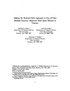
LIST OF FIGURES 1
Network transformation to remove node cost and capacity . . . . . . . . . .
5
2
A MCNF example problem . . . . . . . . . . . . . . . . . . . . . . . . . . .
7
3
Block angular structure of the example problem in Figure 2 . . . . . . . . .
8
4
Illustration of arc adjacency lists, and subgraphs H([2, 4]), H([1, 3] ∪ 5) . .
75
5
Solving a 3 pairs shortest path problem on a 5-node graph by Algorithm DLU 1(Q) . . . . . . . . . . . . . . . . . . . . . . . . . . . . . . . . . . . . .
78
6
Augmented graph after procedure G LU . . . . . . . . . . . . . . . . . . . .
80
7
Solving a 3 pairs shortest path problem on a 5-node graph by Algorithm DLU 2(Q) . . . . . . . . . . . . . . . . . . . . . . . . . . . . . . . . . . . . .
96
8
Illustration of procedure G LU on a small example . . . . . . . . . . . . . .
118
9
An example of all shortest paths to node 3 . . . . . . . . . . . . . . . . . . .
119
10
Generic primal-dual method for arc-path form of multicommodity flow problem156
11
Illustraion on how to obtain θk∗ for commodity k . . . . . . . . . . . . . . .
159
12
Key variable decomposition method for solving the RPP . . . . . . . . . . .
167
13
A small ODMCNF example and its RPP formulation . . . . . . . . . . . . .
169
14
Infinite iterations of key path swapping due to dual degeneracy . . . . . . .
170
xiv
SUMMARY
The shortest path problem is a classic and important combinatorial optimization problems. It often appears as a subproblem when solving difficult combinatorial problems like multicommodity network flow (MCNF) problems. Most shortest path algorithms in the literature are either to compute the 1-ALL single source shortest path (SSSP) tree, or to compute the ALL-ALL all pairs shortest paths (APSP). However, most real world applications require only multiple pairs shortest paths (MPSP), where the shortest paths and distances between only some specific pairs of origindestination nodes in a network are desired. The traditional single source shortest path (SSSP) and all pairs shortest paths (APSP) algorithms may do unnecessary computations to solve the MPSP problem. We survey and summarize many shortest path algorithms, and discuss their pros and cons. We also investigate the Least Squares Primal-Dual method, a new LP algorithm that avoids degenerate pivots in each primal-dual iteration, for solving 1-1 and 1-ALL shortest path problems with nonnegative arc lengths, show its equivalence to the classic Dijkstra’s algorithm, and compare it with the original primal-dual method. We propose two new shortest path algorithms to save computational work when solving the MPSP problem. Our MPSP algorithms are especially suitable for applications with fixed network topology but changeable arc lengths. We discuss the theoretical details and complexity analyses. We test several implementations of our new MPSP algorithms extensively and compare them with many state-of-the-art SSSP algorithms for solving many families of artificially generated networks and a real Asia-Pacific flight network. Our MPSP computational experiments show that there exists no ”killer” shortest path algorithm. Our algorithms have better performance for dense networks, but become worse for larger networks. Although they do not have best performance for the artificially generated graphs, they seem to be competitive for the real Aisa-Pacific flight network.
xv
We provide an extensive survey on both the applications and solution methods for MCNF problems in this thesis. Among those methods, we investigate the combination of the primal-dual algorithm with the key path decomposition method. In particular, to efficiently solve the restricted primal problem (RPP) in each primal-dual iteration, we relax the nonnegativity constraints for some set of basic variables, which makes the relaxed RPP smaller and easier to solve since the convexity constraint will be implicitly maintained. We implement our new primal-dual key path method (KEY), propose new methods to identify max step length, and suggest perturbation methods to avoid degenerate pivots and indefinite cycling problems caused by primal and dual degeneracy. We perform limited computational experiments to compare the running time of the generic primal-dual (PD) method, the Dantzig-Wolfe (DW) decomposition method, and the CPLEX LP solver that solves the node-arc form (NA) of the MCNF problems, with our method KEY. Observations from the computational experiments suggest directions for better DW implementation and possible remedies for improving PD and KEY.
xvi
CHAPTER I
INTRODUCTION TO MULTICOMMODITY NETWORK FLOW PROBLEMS
In this chapter, we first describe an air cargo flow problem in the Asia Pacific region. It is this problem that motivates our research. Because the problem can be modeled as a multicommodity network flow (MCNF) problem, we then introduce many MCNF related research topics and applications. Finally, we review different MCNF formulations and outline this thesis.
1.1
Asia Pacific air cargo system
Air cargo is defined as anything carried by aircraft other than mail, persons, and personal baggage. When an enterprise has facilities in its supply chain located in several different regions, efficient and reliable shipping via air is a crucial factor in its competitiveness and success. For example, many international electronics companies currently practice just-intime manufacturing in which components are manufactured in China, Malaysia, Indonesia, Vietnam, or the Philippines, assembled in Taiwan, Japan or Singapore, and shipped to Europe and America. The Asia Pacific region is expected to have the largest airfreight traffic in the next decade [177] due to the growth of Asia Pacific economies. In particular, China has drawn an increasing amount of investment from all over the world due to its cheap manpower and land. Many enterprises have moved their low-end manufacturing centers to China. Most China-made semifinished products are shipped to facilities in other Asian countries for key part assembly, and then sent out worldwide for sale. The increasing need for faster air transportation drives the construction of larger and more efficient air facilities in the Asia Pacific region. New airports such as Chek Lap Kok airport (Hong Kong), Kansai airport (Osaka, Japan), Inchon airport (Seoul, Korea),
1
Table 1: Division of Asia Pacific into sub regions Region Central Asia South Asia Northeast Asia Southeast Asia South Pacific
Countries in the Region Kazakhstan, Kyrgyzstan, Tajikistan, Turkmenistan, Uzbekistan Afghanistan, Bangladesh, Bhutan, India, Maldives, Nepal, Pakistan, Sri Lanka China, Hong Kong, Japan, Korea (Democratic People’s Republic), Korea (Republic of), Macau, Mongolia, Russian Federation (East of Urals), Taiwan Brunei Darussalam, Cambodia, Indonesia, Lao (Peoples’ Democratic Republic), Malaysia, Myanmar, Philippines, Singapore, Thailand, Vietnam America Samoa, Australia, Christmas Island, Cocos (Keeling) Islands, Cook Islands, Fiji, French Polynesia, Guam, Kiribati, Marshall Islands, Micronesia, Nauru, New Caledonia, New Zealand, Niue, Norfolk Island, Northern Mariana Islands, Palau, Papua New Guinea, Pitcairn, Samoa, Solomon Islands, Tokelau, Tonga, Tuvalu, US Minor Outlying Islands, Vanuatu, Wallis and Futuna Islands
Bangkok airport (Thailand), and Pudong airport (Shanghai, Chian) have been constructed. Other airports such as Changi airport (Singapore), Narita airport (Tokyo, Japan), and Chiang-Kai-Shek airport (Taipei, Taiwan) have built new terminals or runways to be able to handle increased air traffic. A more thorough introduction to the air cargo system in the Asia Pacific region can be found in Bazaraa et al. [39]. This thesis is motivated by a study of the Asia Pacific air cargo system. We will describe an Asia Pacific flight network, and give a mathematical model for the air cargo system which corresponds to a multicommodity network flow (MCNF) model. 1.1.1
Asia Pacific flight network
The Asia Pacific region can be divided into five sub-regions as shown in Table 1. Our research focuses on Northeast and Southeast Asia. Our Asia Pacific flight network (AP-NET) contains two types of nodes: center nodes that represent major cities (or airports) in the Northeast and Southeast Asia regions, and rim nodes that represent major cities in other regions. Arcs represent flight legs between center cities and center/rim cities. Based on data from the Freight Forecast [176], Air Cargo Annual [174], and Asia Pacific Air Transport Forecast [175] published by IATA, we selected 11 center countries (see Table 2) and 20 rim countries (see Table 3). The center countries are the Northeast and Southeast Asian countries that contribute the most intra and inter-regional air cargo traffic. The rim countries are those countries outside the region that have large air cargo traffic with the center countries. 2
Table 2: Center countries and cities of the AP filght network center country China
Hong Kong Indonesia Japan
Korea Malaysia Philippines Singapore Taiwan Thailand Viet Nam
center city name Beijing, Dalian, Guangzhou, Kunming, Qingdao, Shanghai, Shenyang, Shenzhen, Tianjin, Xi An, Xiamen Hong Kong Denpasar Bali, Jakarta, Surabaya Fukuoka, Hiroshima, Kagoshima, Komatsu, Nagoya, Niigata, Okayama, Okinawa, Osaka, Sapporo, Sendai, Tokyo Cheju, Pusan, Seoul Kota Kinabalu, Kuala Lumpur, Kuching, Langkawi, Penang Cebu, Manila, Subic Bay Singapore Kaohsiung, Taipei Bangkok, Chiang Mai, Hat Yai, Phuket Hanoi, Ho Chi Minh City
Table 3: Rim countries and cities of the AP filght network rim country Australia Bahrain Canada Denmark Finland France Germany Greece India Italy Netherlands New Zealand Pakistan Russian Federation Sri Lanka Switzerland Turkey United Arab Emirates United Kingdom USA
rim city name Adelaide, Avalon, Brisbane, Cairns, Darwin, Melbourne, Perth, Sydney Bahrain Toronto, Vancouver Copenhagen Helsinki Paris Frankfurt, Munich Athens Bangalore, Calcutta, Chennai, Delhi, Hyderabad, Mumbai Milan, Rome Amsterdam Auckland, Christchurch Islamabad, Karachi, Lahore Khabarovsk, Moscow, Novosibirsk, St Petersburg, Ulyanovsk Colombo Zurich Istanbul Abu Dhabi, Dubai, Sharjah London, Manchester Anchorage, Atlanta, Boston, Chicago, Dallas/Fort Worth, Detroit, Fairbanks, Honolulu, Houston, Kona, Las Vegas, Los Angeles, Memphis, Minneapolis/St Paul, New York, Oakland, Portland, San Francisco, Seattle, Washington
3
For our case study, we use the OAG MAX software package, which provides annual worldwide flight schedules for more than 850 passenger and cargo airlines, to build a monthly flight schedule of all jet non-stop operational flights between 48 center cities and 64 rim cities in September 2000. AP-NET contains 112 nodes and 1038 arcs, where each node represents a chosen city and each arc represents a chosen flight. Among the 1038 arcs, 480 arcs connect center cities to center cities, 277 arcs connect rim cities to center cities, and 281 arcs connect center cities to rim cities. We do not include the flights between rim cities in this model since we are only interested in the intra and inter-regional air cargo flows for the center nodes. 1.1.2
An air cargo mathematical model
The air cargo flow problem AP-NET is, in fact, a multicommodity network flow problem. In particular, given a monthly air cargo demand/supply data for both the center and rim nodes that have to be shipped via the flight legs (arcs) in AP-NET, then each commodity is a specific product for a specific origin-destination (OD) pair. Let cl,k i,j denote the unit flow cost of shipping product l from origin sk to destination tk (i.e. OD pair k) on flight leg (i, j), and ulij denote the capacity of shipping product l on flight leg (i, j). Each airport i has unit transshipment cost cli and transshipment capacity uli for product l (see Figure 1 (a)). To eliminate the node cost and capacity, we can perform a node splitting procedure as in Figure 1 (b). In particular, suppose node i has to receive Bil1 ,k1 units of import cargo demand l1 from node sk1 , and send Bil2 ,k2 units of export cargo supply l2 to node tk2 . We can split node i into four nodes: an import node i1 for receiving the import cargo, a demand node i2 for receiving Bil21 ,k1 units of local import cargo, a supply node i3 for sending Bil32 ,k2 units of local export cargo, and an export node i4 for sending the export cargo. Suppose the original network has |N | nodes and |A| arcs. Then, the new network will have 4 |N | nodes and |A| + 3 |N | arcs. The transshipment cost and capacity of node i become the cost and capacity of arc (i2 , i3 ). Both arc (i1 , i2 ) and arc (i3 , i4 ) have zero costs and unbounded capacities..
4
l (cl,k ij , uij ) i j
(cli , uli )
cl,k ij : per unit cost of product l from OD pair k on arc (i, j) ulij : capacity of product l on arc (i, j)
(clj , ulj ) cl : per unit transshipment cost of product l in node i i uli : transshipment capacity of product l in node i Local export Bil2 ,k2
h
l (cl,k hi , uhi )
i
Total import
l (cl,k ij , uij )
j
Total export
Local import Bil1 ,k1 (a) Original network for product l
Local export Bil2 ,k2
h
l (cl,k hi , uhi )
Total import
i1
(0, ∞)
(cli , uli ) i3
i2
Transshipment
(0, ∞)
i4
l (cl,k ij , uij )
j
Total export
Local import Bil1 ,k1 (b) Transformed network for product l
Figure 1: Network transformation to remove node cost and capacity In this way, the minimum cost cargo routing problem becomes a minimum cost multicommodity network flow problem. It seeks optimal air cargo routings to minimize the total shipping cost of satisfying the OD demands while not exceeding the airport or flight capacities. Each commodity is defined as a specific product to be shipped from an origin to a destination. If we have all of the parameters (OD demand data for each node, unit shipping and transshipment costs for each commodity on each flight leg and airport, and the capacity of each flight leg and airport), this MCNF problem can be solved to optimality. The sensitivity analysis can give us insight and suggest ways to improve the current Asia Pacific air cargo system. For example, by perturbing the capacity for a specific flight leg or airport, we can determine whether adding more flights or enlarging an airport cargo terminal is profitable, which flight legs are more important, and whether current practices for certain airline or
5
airport are efficient. Similar analyses can be done to determine whether adding a new origin-destination itinerary is worthwhile, or whether increasing the charge on a certain OD itinerary is profitable. However, it is difficult to determine those parameters. The flight capacity may be estimated by adding the freight volumes of each aircraft on a certain flight leg. The unit shipping and transshipping cost or revenue is difficult to determine, since it is a function of several variables such as time, distance, product type and OD itinerary (including the flight legs and airports passed). The transshipment capacity for a cargo terminal is also difficult to estimate since it is variable and dynamic. We may first treat it as unbounded and use the optimal transshipment flow to judge the utility of cargo terminals. Correctly estimating these parameters is itself a challenging research topic. This thesis, on the other hand, focuses on how to solve the MCNF problem more efficiently, given all these parameters.
1.2
MCNF problem description
The multicommodity network flow problem is defined over a network where more than one commodity needs to be shipped from specific origin nodes to destination nodes while not violating the capacity constraints associated with the arcs. It extends the single commodity network flow (SCNF) problem in a sense that if we disregard the bundle constraints, the arc capacity constraints that tie together flows of different commodities passing through the same arc, a MCNF problem can be viewed as several independent SCNF problems. In general, there are three major MCNF problems in the literature: the max MCNF problem, the max-concurrent flow problem, and the min-cost MCNF problem. The max MCNF problem is to maximize the sum of flows for all commodities between their respective origins and destinations. The max-concurrent flow problem is a special variant of the max MCNF problem which maximizes the fraction (throughput) of the satisfied demands for all commodities. In other words, the max concurrent flow problem maximizes the fraction z for which the min-cost the MCNF problem is feasible if all the demands are multiplied by z. The min-cost MCNF problem is to find the flow assignment satisfying the demands of all commodities with minimum cost without violating the capacity constraints on all arcs.
6
(cij , uij )
cij : cost of arc (i, j) j
i
|N | = 5, |A| = 10, |K| = 3 K 1 : (s1 , t1 ) = (1, 4), B 1 = 6 K 2 : (s2 , t2 ) = (5, 3), B 2 = 4 K 3 : (s3 , t3 ) = (3, 1), B 3 = 8
(3,6)
uij : capacity of arc (i, j) (2,9)
(1,7)
1 (1,5) 2 (2,7) 3 (7,4) 4 (3,3) 5
origins, destinations, and demands of three commodities
(3,10)
(2,6)
(6,1)
Figure 2: A MCNF example problem This dissertation will focus on min-cost MCNF problem. Hereafter, when we refer to the MCNF problem, we mean the min-cost MCNF problem. The existence of the bundle constraints makes MCNF problems much more difficult than SCNF problems. For example, many SCNF algorithms exploit the single commodity flow property in which flows in opposition direction on an arc could be canceled out. In MCNF problems, flows do not cancel if they are different commodities. The max-flow min-cut theorem of Ford and Fulkerson [116] in SCNF problems guarantees that the maximum flow is equal to the minimum cut. Furthermore, with integral arc capacities and node demands, the maximum flow is guaranteed to be integral. None of these properties can be extended to MCNF, except for several special planar graphs [255, 254, 224, 250], or two-commodity flows with even integral demands and capacities [170, 276, 278]. The total unimodularity of the constraint matrix in the SCNF LP formulation guarantees integral optimal flows in the cases of integral node supplies/demands and arc capacities. This integrality property also can not be extended to MCNF LP formulations. Solving the general integer MCNF problem is N P -complete [194]. In fact, even solving the two-commodity integral flow problem is N P -complete [107]. Since 1960s, MCNF has motivated many research topics. For example, column generation by Ford and Fulkerson [115] was originally designed to solve max MCNF problems, and is still a common technique for solving large-scale LP problems. Seymour [286] proposes the max-flow min-cut matroid and several important matroid theorems by studying multicommodity flow. The nonintegrality property of MCNF spurs much research in integral
7
1 −1 0 −1 0 0 0 0 0 0 0 1 1 0 −1 0 −1 0 0 0 e = −1 0 0 1 1 1 0 −1 −1 0 N 0 0 −1 0 0 0 1 1 0 −1 0 0 0 0 0 −1 0 0 1 1
e Node-arc incidence matrix N e N I
X = e N = e N = ≤ I I
b1 =[ 6 0 0 -6 0 ]T b2 =[ 0 0 -4 0 4 ]T b3 =[ -8 0 8 0 0 ]T u=[ 6 5 9 10 7 7 6 4 1 3 ]T |A|
X=[ x1 x2 x3 ]T , xk ∈ R+ ∀k ∈ K MCNF constraints
Figure 3: Block angular structure of the example problem in Figure 2 LP related to matroids, algorithmic complexity, and polyhedral combinatorics (see [162] for details). The block-angular constraint structure (see Figure 3) of the MCNF constraints serves as a best practice for decomposition techniques such as Dantzig-Wolfe decomposition [88] and Benders decomposition [42], and basis partitioning methods such as generalized upper bounding [213, 167] and key variables [273].
1.3
Applications
MCNF models arise in many real-world applications. Most of them are network routing and network design problems. 1.3.1
Network routing
1.3.1.1
Message routing in Telecommunication:
Consider each requested OD pair to be a commodity. The problem is to find a min-cost flow routing for all demands of requested OD pairs while satisfying the arc capacities. This appears often in telecommunication. For example, message routing for many OD pairs [36, 237], packet routing on virtual circuit data network [221] (all of the packets in a session are transmitted over exactly one path between the OD to minimize the average number of packets in the network), or routing on a ring network [288] (any cycle is of length n), are
8
MCNF problems. 1.3.1.2
Scheduling and routing in Logistics and Transportation:
In logistics or transportation problems, commodities may be objects such as products, cargo, or even personnel. The commodity scheduling and routing problem is often modeled as a MCNF problem on a time-space network where a commodity may be a tanker [41], aircraft [166], crew [60], rail freight [16, 78, 210], or Less-than Truck-Load (LTL) shipment [109, 38]. Golden [144] gives a MCNF model for port planning that seeks optimal simultaneous routing where commodities are export/import cargo, nodes are foreign ports (as origins), domestic hinterlands (as destinations) and US ports (as transshipment nodes), and arcs are possible routes for cargo traffic. Similar problems appear in grain shipment networks [9, 31]. A disaster relief management problem is formulated as a multicommodity multimodal network flow problem with time windows by Haghani and Oh [164] where commodities (food, medical supplies, machinery, and personnel) from different areas are to be shipped via many modes of transportation (car, ship, helicopter,...,etc.) in the most efficient manner to minimize the loss of life and maximize the efficiency of the rescue operations. 1.3.1.3
Production scheduling and planning:
Jewell [180] solves a warehousing and distribution problem for seasonal products by formulating it as a MCNF model where each time period is a transshipment node, one dummy source and one dummy sink node exist for each product, and arcs connect from source nodes to transshipment nodes, earlier transshipment nodes to later transshipment nodes, and transshipment nodes to sink nodes. Commodities are products to be shipped from sources to sinks with minimum cost. D’Amours et al. [84] solve a planning and scheduling problem in a Symbiotic Manufacturing Network (SMN) for a multiproduct order. A broker receives an order of products in which different parts of the products may be manufactured by different manufacturing firms, stored by some storage firms, and shipped by a few transportation firms between manufacturing firms, storage firms and customers. The problem is to design a planning
9
and scheduling bidding scheme for the broker to make decisions on when the bids should be assigned and who they should be assigned to, such that the total cost is minimized. They propose a MCNF model where each firm (manufacturing or storage) at each period represents a node, an arc is either a possible transportation link or possible manufacturing (storage) decision, and a commodity represents an order for different product. Aggarwal et al. [1] use a MCNF model to solve an equipment replacement problem which determines the time and amount of the old equipments to be replaced to minimize the cost. 1.3.1.4
Other routing:
• VLSI design [61, 279, 270, 8]: Global routing in VLSI design can be modeled as an origin-destination MCNF problem where nodes represent collections of terminals to be wired, arcs correspond to the channels through which the wires run, and commodities are OD pairs to be routed. • Racial balancing of schools [77]: Given the race distribution of students in each community, and the location, capacity and the ethnic composition requirements of each school, the problem is to seek an assignment of students to schools so that the ethnic composition at each school is satisfied, no student travels more than a specified number of minutes per day, and the total travel time for students to school is minimized. This is exactly a MCNF problem in the sense that students of the same race represent the same commodity. • Caching and prefetching problems in disk systems [6, 7]: Since the speed of computer processors are much faster than memory access, caching and prefetching are common techniques used in modern computer disk systems to improve the performance of their memory systems. In prefetching, memory blocks are loaded from the disk (slow memory) into the cache (fast memory) before actual references to the blocks, so the waiting time is reduced in accessing memory from the disk. Caching tries to keep actively referenced memory blocks in fast memory. At any time, at most one fetch operation is executed. Albers and Witt [7] model this problem as a min-cost 10
MCNF problem that decides when to initiate a prefetch, and what blocks to fetch and evict. • Traffic equilibrium [215, 110]: The traffic equilibrium law proposed by Wardrop [303] states that at equilibrium, for each origin-destination pair, the travel times on all routes used are equal, and are less than the travel times on all nonused routes. Given the total demand for each OD pair, the equilibrium traffic assignment problem is to predict the traffic flow pattern on each arc for each OD pair that follows Wardrop’s equilibrium law. It can be formulated as a nonlinear MCNF problem where the bundle constraints are eliminated but the nonlinear objective function is designed to capture the flow congestion effects. • Graph Partitioning [285]: The graph partitioning problem is to partition a set of nodes of a graph into disjoint subsets of a given maximal size such that the number of arcs with endpoints in different subsets is minimized. It is an N P -hard problem. Based on a lower bounding method for the graph bisection problem, which corresponds to a MCNF problem, Sensen [285] proposes three linear MCNF models to obtain lower bounds for the graph partitioning problem. He then uses branch-andbound to compute the exact solution. Similarly, many N P -hard problems such as min-cut linear arrangement, crossing number, minimum feedback arc set, minimum 2D area layout, and optimal matrix arrangement for nested disection can be approximately solved by MCNF algorithms [217, 204, 206, 219]. 1.3.2
Network design
Given a graph G, a set of commodities K to be routed according to known demands, and a set of facilities L that can be installed on each arc, the capacitated network design problem is to route flows and install facilities at minimum cost. This is a MCNF problem which involves flow conservation and bundle constraints plus some side constraints related to the installation of the new facilities. The objective function may be nonlinear or general discontinuous step-increasing [124]. 11
Problems such as the design of a network where the maximum load on any edge is minimized [51] or the service quality and survivability constraints are met with minimum cost of additional switches/transport pipes in ATM networks [53] appear often in the telecommunication literature. Bienstock et al. use metric inequalities, aggregated formulations [50] and facet-defining inequalities [52] to solve capacitated survivable network design problems. Gouveia [152] discusses MCNF formulations for a specialized terminal layout problem which seeks a minimum spanning tree with hop constraints (a limit on the number of hops (links) between the computer center and any terminal in the network). Maurras et al. [232, 163] study network design problems with jump constraints (i.e., each path has no more than a fixed number of arcs). Girard and Sans`o [133] show that the network designed using a MCNF model significantly improves the robustness of the heuristic solutions at a small cost increase. Gendron et al. [130] write a comprehensive survey paper in multicommodity capacitated network design. Similar problems also appear in transportation networks, such as locating vehicle depots in a freight transportation system so that the client demands for empty vehicles are satisfied while the depot opening operating costs and other transportation costs are minimized. Crainic et al. [80] have solved this problem by various methods such as branch-and-bound [82] and its parallelization [129, 56], dual-ascent [81], and tabu-search [83]. Crainic also writes a survey paper [79] about service network design in freight transportation. In fact, these problems are facility location problems. Geoffrion and Graves [132] model a distribution system design problem as a fixed charge MCNF problem. More MCNF models for facility location are surveyed by Aikens [5].
1.4
Formulations
Let N denote the set of all nodes in G, A the set of all arcs, and K the set of all commodities. For commodity k with origin sk and destination tk , ckij represents its per unit flow cost on arc (i, j) and xkij the flow on arc (i, j). Let bki be the supply/demand at node i, and B k be the total demand units of commodity k. Let uij be the arc capacity on arc (i, j). Without loss of generality, we assume each unit of each commodity consumes one unit of capacity
12
from each arc on which it flows. 1.4.1
Node-Arc form
The node-arc form of MCNF problem is a direct extension of the conventional SCNF formulation. It can be formulated as follows: min
X X
ckij xkij = Z ∗ (x)
(Node-Arc)
k∈K (i,j)∈A
s.t.
X
(i,j)∈A
X
xkij −
(j,i)∈A
X
k∈K
xkji = bki ∀i ∈ N , ∀k ∈ K
(1.1)
xkij ≤ uij ∀(i, j) ∈ A (bundle constraints)
(1.2)
xkij ≥ 0 ∀(i, j) ∈ A, ∀k ∈ K where bki = B k if i = sk , bki = −B k if i = tk , and bki = 0 if i ∈ N \{sk , tk }. This formulation has |K||A| variables and |N ||K| + |A| nontrivial constraints. 1.4.2
Arc-Path form
First suggested by Tomlin [297], the arc-path form of the min-cost MCNF problem is based on the fact that any network flow solution can be decomposed into path flows and cycle flows. Under the assumption that no cycle has negative cost, any arc flow vector can be expressed optimally by simple path flows. For commodity k, let P k denote the set of all possible simple paths from sk to tk , fp the units of flow on path p ∈ P k , and P Cpc the cost of path p using ckij as the arc costs. δap is a binary indicator which equals to 1 if path p passes through arc a, and 0 otherwise. It can be formulated as follows: min
X X
k∈K
P Cpc fp = Z ∗ (f )
(Arc-Path)
p∈P k
s.t.
X
p∈P k
X X
k∈K p∈P k
fp = 1 ∀k ∈ K
(B k δap )fp ≤ ua ∀a ∈ A (bundle constraints) fp ≥ 0 ∀p ∈ P k , ∀k ∈ K 13
(1.3) (1.4)
Inequalities (1.4) are the bundle constraints, and (1.3) are the convexity constraints which force the optimal solution for each commodity k to be a convex combination of some simple paths in P k . Since we only consider the LP MCNF problem in this dissertation, the optimal solution can be fractional. For the binary MCNF problem where each commodity can only be shipped on one path, fp will be be binary variables. P |P k | variables and |K| + |A| nontrivial constraints. This formulation has k∈K
1.4.3
Comparison of formulations
When commodities are OD pairs, |K| may be O(|N |2 ) in the worst case. In such case, the node-arc form may have O(|N |3 ) constraints which make its computations more difficult and memory management less efficient. The arc-path formulation, on the other hand, has at most O(|N |2 ) constraints but exponentially many variables. The problem caused by a huge number of variables can be resolved by column-generation techniques. In particular, when using the revised simplex P method to solve the arc-path form, at most |K| + |A| of the |P k | variables are positive k∈K
in any basic solution. In each iteration of the revised simplex method, a shortest path
subproblem for each commodity can be solved to find a new path for a simplex pivot-in operation if it corresponds to a nonbasic column with negative reduced cost. Dantzig-Wolfe (DW) decomposition is a common technique used to solve problems with block-angular structure. The algorithm decomposes the problem into two smaller sets of problems, a restricted master problem (RMP) and k subproblems, one for each commodity. It first solves the k subproblems and uses their basic columns to solve the RMP to optimality. Then it uses the dual variables of the RMP to solve the k subproblems, which produce nonbasic columns with negative reduced cost to be added to the RMP. The procedures are repeated until no more profitable columns are generated for the RMP. More details about DW will be discussed in Section 2.3.2. Jones et al. [187] investigate the impact of formulation on Dantzig-Wolfe decomposition for the MCNF problem. Three formulations: origin-destination specific (ODS), destination specific (DS), and product specific (PS) are compared in Table 4 where shortest path,
14
shortest path tree, and min-cost network flow problems are the subproblems for ODS, DS, and PS respectively. Table 4: Comparison of three DW formulations [187] subproblem∗ RMP size RMP sparsity∗∗ number of master iterations number of commodities convergence rate *: A Â B means A is harder than B ; **:
ODS ≺ DS ≺ P S ODS > DS > P S ODS Â DS Â P S ODS < DS < P S ODS À DS > P S ODS > DS > P S A Â B means A is sparser than B
Although the ODS form has a larger RMP and more subproblems (due to more commodities), it has a sparser RMP, easier subproblems, and better extreme points produced which contribute to faster convergence than other forms. Knowing this fact, our solution methods to the min-cost ODMCNF problem will be path-based techniques.
1.5
Contributions and thesis outline
We consider the following to be the major contributions of this thesis: • We survey and summarize MCNF problems and algorithms that have appeared in the last two decades. • We survey and summarize shortest path algorithms that have appeared in the last five decades. • We observe the connection between a new shortest path algorithm and the well-known Dijkstra’s algorithm. • We propose three new multiple pairs shortest path algorithms, discuss their theoretical properties, and analyze their computational performance. • We give two new MCNF algorithms, and compare their computational performance with two standard MCNF algorithms. 15
This thesis has six chapters. Chapter 1 discusses MCNF applications and their formulations. Chapter 2 surveys MCNF solution techniques from the literature. Since our approaches require us to solve many multiple pairs shortest paths (MPSP) problems, we will propose new efficient MPSP algorithms. Chapter 3 first reviews the shortest path solution techniques that have appeared in the last five decades, and then introduces a new shortest path method which uses the nonnegative least squares (NNLS) technique in the primal-dual (PD) algorithmic framework, and discusses its relation to the well-known Dijkstra’s algorithm. Chapter 4 discusses the theoretical details of our new MPSP algorithms. Chapter 5 presents the computational performance of our new MPSP algorithms. Finally, Chapter 6 illustrates our primal-dual MCNF algorithms, analyzes their computational performance, and suggests new techniques to improve the algorithms. Chapter 7 concludes this thesis and suggests future research.
16
CHAPTER II
SOLUTION METHODS FOR MULTICOMMODITY NETWORK FLOW PROBLEMS
In this chapter, we try to summarize most of the solution techniques that have appeared in the literature, especially those which appeared after 1980. Due to the special block-angular structure of MCNF problems, many special solution methods have been suggested in the literature. Basis partitioining methods partition the basis in a way such that computing the inverse of the basis is faster. Resource-directive methods seek optimal capacity allocations for commodities. Price-directive methods try to find the optimal penalty prices (dual variables) for violations of the bundle constraints. Primal-dual methods raise the dual objective while maintaining complementary slackness conditions and will be discussed in more detail in Chapter 6. In the last two decades, many new methods such as approximation methods, interior-point methods and their parallelization have been proposed. Although the convex or integral MCNF problems are not the main interests of this dissertation, we still summarize recent progress in these topics.
2.1
Basis partitioning methods
The underlying idea of basis partitioining methods is to partition the basis so that the special network structure can be maintained and exploited as much as possible to make the inversion of the basis more efficient. Hartman and Lasdon [167] propose a Generalized Upper Bounding (GUB) technique which is a specialized simplex method whose only nongraphic operations involve the inversion of a working basis with dimension equal to the number of currently saturated arcs. Other basis partitioning methods based on GUB techniques have also been suggested by McCallum [238] and Maier [228]. Grigoriadis and White [156, 155] observe that, in practice, the number of active bundle constraints in the optimal solution are considerably smaller than the number of capacitated
17
arcs. Therefore they partition the constraints into two groups: current and secondary constraints. Using the dual simplex method with Rosen’s partition technique [273], they iteratively solve sequences of LPs that use only updated current constraints. These LPs do not need to be solved to optimality. The algorithm only requires a basis change when dual feasibility is maintained and the objective value decreases. Kennington [200] implements the primal partitioning methods of Saigal [277] and Hartman and Lasdon [167]. His implementation of basis partitioning methods are computationally inferior to resource-directive subgradient methods. EMNET, developed by McBride [233] and based on the factorization methods (variants of basis partition methods) of Graves and McBride [154], is designed to quickly solve LP problems with network structure and network problems with side constraints. Combined with other techniques such as resource-directive heuristics and price-directive column generation, they conclude that basis partitioning methods are computationally efficient. In particular, McBride and Mammer [236] use a capacity allocation heuristic to produce a hot-start basis for EMNET which shortens the computational time. McBride [235] uses a reource-directive decomposition heuristic to control the size of the working inverse and dramatically reduce the solution time for MCNF problems with many side constraints. Mamer and McBride [229, 237] also apply column generation techniques of DW decomposition to solve message routing problems and find a dramatic reduction in the number of pivots needed. The combination of EMNET and column generation shows a larger reduction in computation time than direct application of EMNET. A similar specialized simplex algorithm has also been proposed by Detlefsen and Wallace [92]. Their paper addresses more details of the network interpretation of basis inversion. Independent of the number of commodities, their working basis has dimesion at most equal to the number of arcs in the network, which seems to be suitable for telecommunication problems that often have a large number of commodities. Castro and Nabona [70] implement a MCNF code named PPRN to solve min-cost MCNF problems which have a linear or nonlinear objective function and additional linear side constraints. PPRN is based on a primal partitioning method using Murtagh and Saunders’
18
[246] strategy of dividing the variables into three sets: basic, nonbasic and superbasic. Farvolden et al. [109] partition the basis of the master problem using the arc-path form in DW decomposition. Their techniques isolate a very sparse and near-triangular working basis of much smaller dimension, and identify nine possible types of simplex pivots that can be done by additive and network operations to greatly improve the efficiency. Such techniques are later used to solve a MCNF problem with jump constraints (i.e., commodities can not be shipped along more than a fixed number of arcs) [232] and further refined by Hadjiat et al. [163] so that the dimension of the working basis is at most equal to the number of arcs in the network (almost half the size of the working matrix of [109]).
2.2
Resource-directive methods
k for each commodity k so that Suppose on each arc (i, j) we have assigned capacity rij P k rij ≤ uij is satisfied. Then the original problem is equivalent to the following resource k∈K
allocation problem (RAP) that has a simple constraint structure but complex objective
function: min
X
z k (rk ) = z(r)
(RAP)
k∈K
X
s.t.
k∈K
k rij ≤ uij ∀(i, j) ∈ A
k 0 ≤ rij ≤ uij ∀(i, j) ∈ A, ∀k ∈ K
For each commodity k, z k (rk ) can be obtained by solving the following single commodity min-cost network flow subproblem. min
X
ckij xkij = z k (rk )
(i,j)∈A
s.t.
X
(i,j)∈A
xkij −
X
(j,i)∈A
xkji = bki ∀i ∈ N
k 0 ≤ xkij ≤ rij ∀(i, j) ∈ A
It can be shown that the objective function z(r) is piecewise linear on the feasible set of the capacity allocation vector r. There are several methods in the literature to solve
19
the RAP such as tangential approximation [131, 132, 201], feasible directions [201], and the subgradient method [131, 161, 153, 168, 199]. Shetty and Muthukrishnan [289] give a parallel projection algorithm which parallelizes the procedure of projecting new resource allocations in the resource-directive methods.
2.3
Price-directive methods
Price-directive methods are based on the idea that by associating the bundle constraints with ”correct” penalty functions (dual prices, or Lagrange multipliers), a hard MCNF problem can be decomposed into k easy SCNF problems. 2.3.1
Lagrange relaxation (LR)
Lagrange relaxation dualizes the bundle constraints using a Lagrangian multiplier π ≥ 0 so that the remaining problem can be decomposed into k smaller min-cost network flow problems. In particular, min
X
k∈K
s.t.
ck x k +
X
πa (
a∈A
X
k∈K
xka − ua ) = L(π)
e xk = bk , ∀k ∈ K N x≥0
e is the node-arc incidence matrix. The Lagrangian dual problem seeks an optimal where N
π ∗ for L∗ = max L(π). This is a nondifferentiable optimization problem (NDO) having the π≥0
format max{ϕ(y) : y ∈ Y } where ϕ is a concave nondifferentiable function and Y is a convex |A|
nonempty subset of R+ . Subgradient methods are common techniques for determining the Lagrange multipliers. They are easy to implement but have slow convergence rates. They usually do not have a good stopping criterion, and in practice usually terminate when a predefined number of iterations or nonimproving steps is reached. Papers regarding subgradient methods have been listed in Section 2.2. Chapter 16 and 17 of [3] also present illustrative examples. Bundle methods are designed to solve general NDO problems and thus are suitable for solving the Lagrangian dual problems. In particular, let g(y 0 ) denote a supergradient of ϕ
20
at y 0 , that is, ϕ(y) ≤ ϕ(y 0 ) + g(y − y 0 ) for all y in Y . Define the bundle to be a set β that contains all ϕ(yi ) and g(yi ) generated in previous iterations. The generic bundle method starts with an initial y 0 and β and searches for a tentative ascent direction d. It tentatively updates y 00 = y 0 + θd. If the improvement ϕ(y 00 ) − ϕ(y 0 ) is large enough, the solution y 0 will move to y 00 . Otherwise, it adds ϕ(y 00 ) and g(y 00 ) to the bundle β so that next iteration may give a better tentative ascent direction. In general, bundle methods converge faster and are more robust than subgradient methods. Frangioni’s Ph.D. dissertation [118] is a rich resource for the bundle method and its application to solving MCNF problems. Gendron et al. [130] use the bundle method to solve a multicommodity capacitated fixed charge network design problem. Cappanera and Frangioni [59] give its parallelization together with discussion on other parallel price-directive approaches. Both the subgradient methods and bundle methods are dual based techniques, in which usually extra effort has to be made to obtain a primal feasible solution. Next we will introduce methods that improve the primal feasible solution and compute the Lagrangian multipliers by solving a LP in each iteration. 2.3.2
Dantzig-Wolfe decomposition (DW)
As previously mentioned in Section 1.4.3, here we illustrate more details about the DW procedures using the arc-path form. The primal path formulation is as follows: min
X X
P Cpc fp = ZP∗ (f, s)
(P PATH)
k∈K p∈P k
X
s.t.
p∈P k
X X
k∈K
p∈P k
fp = 1 ∀k ∈ K
(B k δap )fp ≤ ua ∀a ∈ A fp ≥ 0 ∀p ∈ P k , ∀k ∈ K
21
(2.1) (2.2)
whose dual is max
X
X
σk +
(D PATH)
a∈A
k∈K
s.t. σk +
∗ ua (−πa ) = ZD (π, σ)
X
a∈A
B k δap (−πa ) ≤ P Cpc ∀p ∈ P k , ∀k ∈ K
(2.3)
πa ≥ 0 ∀a ∈ A σk : free ∀k ∈ K where σk are the dual variables for the convexity constraint (2.1) and −πa are the dual variables for the bundle constraints (2.2). The complementary slackness (CS) conditions are: (−πa )(
X X
k∈K p∈P K
(B k δap )fp − ua ) = 0 ∀a ∈ A X
(CS.1)
fp − 1) = 0 ∀k ∈ K
(CS.2)
fp (P Cpc+π − σk ) = 0 ∀p ∈ P k , ∀k ∈ K
(CS.3)
σk (
p∈P K
P
B k δap (ca + πa ) and ca is the original cost of arc a. The reduced cost of P k p P k p path p is P Cpc − B δa (−πa ) − σk = B δa (ca + πa ) − σk = P Cpc+π − σk . where P Cpc+π :=
a∈A
a∈A
a∈A
Suppose a feasible but nonoptimal primal solution (f, s) is known. We construct the
RMP which contains the columns associated with positive f and s, solve the RMP to optimality, and obtain its optimal dual solution (σ ∗ , −π ∗ ). This optimal dual solution can ∗
be used to identify profitable columns (i.e. columns with reduced cost P Cpc+π − σk∗ < 0) and add them to construct a new RMP. The procedure for generating new columns is equivalent to solving k subproblems. Each subproblem corresponds to a shortest path ∗ ) as the new problem from sk to tk for a single commodity k. In particular, using (cij + πij ∗
= cost for each arc (i, j), if the length of the shortest path pk∗ for commodity k, P Cpc+π k∗ P k∗ p ∗ ), is shorter than σ ∗ , then we add the column corresponding to path (cij + πij B k δij k (i,j)∈A pk∗ to
the RMP. The algorithm iteratively solves the RMP and generates new columns
until no more columns have negative reduced cost (which guarantees optimality). During the procedure, primal feasibility and complementary slackness are maintained. 22
The DW algorithm stated above can also be viewed as a procedure to identify the optimal dual variables (σ ∗ , −π ∗ ) by solving sequences of smaller LP problems (RMP). Compared to LR, DW spends more time in solving the RMP, but obtains better dual variables. In general, DW requires fewer iterations than LR to achieve optimality. Another advantage of DW is that it always produces primal feasible solutions which can be used as upper bounds in minimization, while its dual objective can be used as a lower bound. LR, on the other hand, usually only guarantees an optimal dual solution and may require extra effort to obtain an optimal primal solution. Unlike the conventional dual-based subgradient methods, the volume algorithm of Barahona and Anbil [24] is an extension of the subgradient methods. It produces approximate primal solutions in DW procedures. The method is similar to the subgradient method and the bundle method introduced in Section 2.3.1, and has the following steps: • Step 0: Given a feasible dual solution −π to the bundle constraint (2.2), we solve |K| subproblems. Each subproblem has the following form: min
X
(ckij + π ij )xkij = Z
k
(Vol(k ))
(i,j)∈A
s.t.
X
(i,j)∈A
xkij −
X
(j,i)∈A
xkji = bki ∀i ∈ N xkij ≥ 0 ∀(i, j) ∈ A
k
Suppose (Vol(k )) has optimal solution xk and optimal objective value Z . |K| P k P Set t = 1, x = [x1 . . . x|K| ]T and Z = Z − uij π ij . k=1
t =u − • Step 1: Compute vij ij
where the step length θ = f
P
(i,j)∈A
t = max{π + θv t , 0} for xkij , and πij ij ij k∈K U B−Z , f is a parameter between 0 and kv t k2
each arc (i, j) 2, and U B is
the upper bound on the objective for P PATH which can be computed by any primal feasible solution. t instead of π For each commodity k, we solve (Vol(k )) using the new πij ij in the
objective function, and obtain its optimal solution xkt and optimal objective value 23
Z kt Set xt = [x1t . . . x|K|t ]T and Z t =
|K| P
k=1
Z kt −
P
(i,j)∈A
t . uij πij
Update x = ηxt + (1 − η)x where η is a parameter between 0 and 1. t for each arc (i, j) and Z = Z t . • Step 2: if Z t > Z then update π ij = πij
Let t = t + 1, and go to Step 1. ¯ ¯ ¯ ¯ P ° t° ¯ ¯ ° ° The algorithm terminates when either v becomes too small or ¯ u π ¯ is smaller ¯(i,j)∈A ij ij ¯ than some threshold value. Suppose Z t ≤ Z for all iterations tc ≤ t ≤ td . In these iterations, the volume algorithm t . In such case, uses the new xkij but the old π ij and Z to compute the new subgradients vij
x = (1 − η)td −tc xtc + (1 − η)td −tc −1 ηxtc +1 + . . . + (1 − η)ηxtd −tc −1 + ηxtd −tc . That is, x is a convex combination of {xtc , . . . , xtd } which is an approximation to the optimal arc flow solution. The basic idea is, given (Z, −π) where −π is a feasible dual variable to the bundle constraint and Z is computed using −π, the volume algorithm moves in a neighborhood of (Z, −π) to estimate the volumes below the faces that are active in the neighborhood; thus better primal solutions are estimated at each iteration. On the other hand, using the conventional subgradient methods, the subgradient v is usually determined by only one active face, and no primal solution can be computed. The volume algorithm has been tested with success in solving some hard combinatorial problems such as crew scheduling problems [25], large scale facility location problems [26, 27], and Steiner tree problems [23]. In [23], the problem is formulated as a non-simultaneous MCNF problem. It is believed that the volume algorithm is advantageous for solving set partitioning-type problems including the MCNF problems. It will be interesting to learn how this new algorithm performs in solving general MCNF problems. To the best of our knowledge, no such work has been done yet. 2.3.3
Key variable decomposition
Based on a primal partitioning method of Rosen [273], Barnhart et al. [36] give a column generation algorithm which is especially suitable for problems with many commodities (OD 24
pairs). In particular, they select a candidate path called a key path, key(k), for each commodity k. After performing some column operations to eliminate key(k) for each k, they obtain the following CYCLE form: min
X X
CCpc fp +
X
M αa = ZC∗ (f, α)
X
s.t.
= 1 ∀k ∈ K
fp
p∈P k
X X
k∈K p∈P k
(CYCLE)
a∈A
k∈K p∈P k
B k (δap − δakey(k) )fp − αa ≤ ua −
X
k∈K
(2.4)
(B k δakey(k) ) ∀a ∈ A
(2.5)
fp ≥ 0 ∀p ∈ P k , ∀k ∈ K αa ≥ 0 ∀a ∈ A c where αa is an artificial variable for each arc a with large cost M , and CCpc = P Cpc −P Ckey(k)
represents the cost of several disjoint cycles obtained by the symmetric difference of path p and key(k). This CYCLE formulation is essentially the same as the P PATH formulation in Dantzig-Wolfe decomposition. The artificial variables with large costs here are used to get an easy initial primal feasible solution for the algorithm. When the number of commodities (OD pairs) is huge, both CYCLE and P PATH will have many constraints, which makes the RMP more difficult. To overcome this computational burden, Barnhart et al. exploit Rosen’s key variable concept which relaxes the nonnegativity constraints for each key path (i.e., it allows fkey(k) to be negative). The RMP can be solved by iteratively solving these easier problems RELAX(i), each of which contains only (1) all of the bundle constraints and (2) the nonnegativity constraints for all variables except the key variables. min
X X
k∈K
s.t.
X X
k∈K
p∈P k
p∈P k
CCpc,i fpi +
X
∗ M αai = ZCR(i) (f, α)
(RELAX(i ))
a∈A
B k (δap − δakey(k,i) )fpi − αai ≤ ua −
X
k∈K
(B k δakey(k,i) ) ∀a ∈ A
fpi ≥ 0 ∀p ∈ P k \ key(k, i), ∀k ∈ K ; fkey(k,i) : free ∀k ∈ K αai ≥ 0 ∀a ∈ A
25
(2.6)
After solving RELAX(i), the algorithm will check the sign of key variables by calculating P i∗ fpi∗ . For those key variables with negative signs, the algorithm will fkey(k,i) = 1− p∈P k \key(k,i)
perform a key variable change operation which replaces the current key variable with a new
one. Among all the positive path variables, the one with the largest value is usually chosen since intuitively that path is more likely to have positive flow in the optimal solution. This algorithm maintains dual feasibility and complementary slackness while trying to achieve primal feasibility (which will be attained when all key variables become nonnegative). Like the subproblems of DW, the subproblems of RELAX(i) are shortest path problems for each commodity k. Suppose in some iteration we solve the RMP of RELAX(i) and obtain the optimal dual solution associated with the bundle constraint (2.6), denoted by ∗
∗
,i c+π ,i −π ∗ . A shortest path pk∗ is generated if its reduced cost P Cpc+π −P Ckey(k,i) < 0. Barnhart k∗
et al. [34, 35] further use a simple cycle heuristic to generate more good columns to shorten the overall computational time. In particular, for commodity k, the symmetric difference of shortest path pk∗ and key path key(k, i) forms several simple cycles. Intuitively, these simple cycles have better potential to contain positive flows since they contribute to both the shortest path pk∗ and the key path key(k, i). Each simple cycle corresponds to a simple column in the RELAX(i) formulation. Suppose pk∗ and key(k, i) form n e simple cycles.
Instead of adding only one column, they add all these n e simple columns at once. Such heuristics do speed up the LP solution procedures.
We will exploit this key variable concept in Section 6.2. 2.3.4
Other price-directive methods
The primal column generation techniques correspond to the dual cutting-plane generation schemes which increasingly refine the polyhedral approximation of the epigraph of the Lagrangian L(π). Goffin et al. [137] propose a specialized analytic center cutting plane method (ACCPM) [136, 18] to solve the nonlinear min-cost MCNF problems. Using a piecewise continuous, smooth, convex and nonseparable linear-quadratic penalty (LQP) function to penalize the overflow of bundle constraints for each arc, Pinar and Zenios [266] design a parallel decomposition algorithm which parallelizes the procedures of solving
26
the nonlinear master problem and independent subproblems in the framework of pricedirective methods. Schultz and Meyer [283] give a price-directive interior-point method using a barrier function (see Section 2.6). Many approximation algorithms are also based on price-directive techniques and will be discussed in Section 2.5. The Section 1.3 of Grigoriadis and Khachiyan [160] cites other old price-directive methods that we omit in this section.
2.4
Primal-dual methods (PD)
The primal-dual method is a dual-ascent LP solution method which starts with a feasible dual solution, and then iteratively constructs a primal feasibility subproblem called the restricted primal problem (RPP) based on the complementary slackness (CS) conditions. It uses the optimal dual solution of RPP to improve the current dual solution if primal infeasibility still exists. The algorithm terminates when all primal infeasibility disappears. Jewell [182, 181] proposes a PD algorithm to solve the min-cost MCNF problem. Given feasible dual variables, he uses the CS conditions to construct a restricted network which can be viewed as |K| layers of single-commodity networks plus some connecting arcs between layers representing the bundle constraints. The RPP becomes a max MCNF problem. He uses a technique similar to the resource-directive methods which first identifies augmenting paths inside each layer until the layer is saturated, and then solves a capacity reallocation problem between layers. His approach requires enumeration of all paths and cycles, which is not efficient. Barnhart and Sheffi [32, 38] present a network-based primal-dual heuristic (PDN) which solves a large-scale MCNF problem that is impractical to solve using other exact solution methods. In each primal-dual iteration of PDN, the RPP is solved by a network-based flow adjustment algorithm (FAA) instead of using conventional LP methods. When the FAA experiences insufficient progress or cycling, the simplex method will be invoked to solve the RP. Given a feasible dual solution, PDN iteratively identifies an admissible set S k which contains arcs with zero reduced cost in the node-arc form for each commodity k, searches for
27
a flow assignment that satisfies the CS conditions using the FAA, and improves the current dual solution if the RPP is solved with positive primal infeasibility. PDN terminates when either the RPP cannot be solved by the FAA or optimality is achieved. In the first case, if the simplex method is invoked but fails due to the huge size of RPP, Barnhart uses a primal solution heuristic [33] that generates feasible primal solutions from the known dual feasible solution. Polak [268] gives a Floyd-Warshall-like algorithm to determine the step length required to improve the dual solution in the PD procedures of solving MCNF problems. More details about PD algorithms will be discussed in Chapter 6.
2.5
Approximation methods
Given a desired accuracy ² > 0, an ²-optimal solution is a solution within (1 + ²) (for minimization problems, or (1 − ²) for maximization problems) of the optimal one. A family of algorithms is called a fully polynomial time approximation scheme (FPTAS) when it computes an ²-optimal solution in time polynomial in the size of problem input and ² −1 . Shahrokhi and Matula [287] present the first combinatorial FPTAS for a special case of the max-concurrent flow problem that has arbitrary demands and uniform capacities. The idea is to start with a flow satisfying the demands but not the bundle constraints, and then iteratively reroute flow to approach optimality. They also use an exponential function of the arc flow as the ”length” of the arc to represent its congestion, so that their algorithm will iteratively reroute flow from longer paths (more congestion) to shorter paths (less congestion). Using different ways for measuring the congestion on arcs and a faster randomized method for choosing flow paths, Klein et al. [205] further improve the theoretical running time. Leighton et al. [218] use the same randomized technique of [205] but a different rerouting scheme to solve a max-concurrent flow problem that has nonuniform integer capacities. Instead of only rerouting a single path of flow as in [287, 205], they solve a min-cost flow problem which takes more time but reroutes more flows and makes greater progress at each iteration. Goldberg [138] and Grigoriadis and Khachiyan [157] independently use different
28
randomized techniques to reduce the randomized algorithmic running time of [218] from a factor of ²−3 to a factor of ²−2 . Radzik [269] achieves the same complexity using a deterministic approximation algorithm. Most of the approximation algorithms mentioned above are designed for max MCNF or max-concurrent flow problems, which can be viewed as packing LPs. In particular, let Pˆ k denote the polytope of all feasible flows for commodity k. Then, the max MCNF S problem can be viewed as packing feasible paths from the polytope Pˆ k subject to the k
bundle constraints. Similarly, the min-cost MCNF problem can be viewed as packing paths subject to bundle and budget constraints. It can be solved by iterations of a separation problem that determines the optimal budget using bisection search [267]. Recently, Grigoriadis and Khachiyan[157, 158], Plotkin et al. [267], Garg and K¨onemann [128, 208], and Young [309] have investigated approximation methods for solving packing and covering problems, especially on applications in the MCNF fields. These algorithms are based on Lagrangian relaxation and can be viewed as randomized potential reduction methods [157, 158]. For example, given a current flow f1 , [267] computes an optimal flow f1∗ (or [157] computes an approximately optimal flow) that uses a ”penalty” potential function as the arc length to represent the violation of bundle constraints, and updates the flow
f2 = (1 − σ)f1 + σf1∗ using some predefined constant σ so that the total ”potential” in the next iteration will be reduced. The length for each arc is usually an exponential function [157, 158, 267, 309] (or a logarithmic function [159]) measuring the congestion (i.e., violation of bundle constraints). While [267, 157] improve the potential by a fixed amount and reroute flows at each iteration, [309] gives an ”oblivious” rounding algorithm which builds the flow from scratch without any flow rerouting operations. The running time of [267] and [309] depend on the the maximum possible ”overflow” of the bundle constraints for points in the S polytope Pˆ k , denoted as the width of the problem. k
Karger and Plotkin [192] combine the approximate packing techniques of [267] and the
flow rerouting order of [269] to give a better deterministic approximation algorithm to solve min-cost MCNF problems. They develop new techniques for solving the ”packing with budget” problems. Such techniques can be used to solve problems with multiple
29
cost measures on the arc flows. Its direct implementation is slow, but a fast practical implementation is proposed by Oldham et al. [256, 139] using techniques from [159, 192, 267] to fine-tune many algorithmic parameters. Garg and K¨onemann [128, 208] propose a simple combinatorial approximation algorithm similar to Young’s [309], which has the most improvement at each iteration using shortest path computations. Fleischer [111] further improves the algorithms of [128] and gives approximation algorithms that have the best running time for solving the max MCNF, max-concurrent flow and min-cost MCNF problems. Grigoriadis and Khachiyan [158] use a 2-phase exponential-function reduction method to solve general block-angular optimization problems. Both phases are resource-sharing S problems. The first phase is to obtain a feasible solution interior to the polytope Pˆ k . The k
second phase uses a modified exponential potential function to optimize on both bundle and flow conservation constraints. Awerbuch and Leighton [19, 20] give deterministic approximation algorithms which use local-control techniques similar to the preflow-push algorithm of Goldberg and Tar-
jan [141, 143]. Unlike previous approximation algorithms that usually relax the bundle constraints and then determine shortest paths or augmenting paths to push flow towards sinks, their algorithms relax the flow conservation constraints and use an ”edge-balancing” technique which tries to send a commodity across an arc (u, v) if node u has more congestion than node v. Based on these edge-balancing methods [19, 20] (denoted as first-order algorithms), Muthukrishnan and Suel [248] propose a second-order distributed flow algorithm which decides the amount of flow to be sent along an arc by a combination of the flow sent on the same arc in previous iteration and the flow determined using the first-order algorithms. Their experiments show a significant improvement in running time compared to the first-order algorithms. Kamath et al. [190, 262] generalize the algorithm of [20] to solve min-cost MCNF problems, but their algorithm is inferior to [192]. Schneur and Orlin [280, 281] present a penalty-based approximation algorithm that solves the min-cost MCNF problems as a sequence of a finite number of scaling phases. In each phase, |K| SCNF problems are solved, one for each commodity. Besides the original 30
linear flow cost ckij xkij , they assign a quadratic penalty term ρe2ij for each arc (i, j) where P k xij −uij , 0} represents the overflow (or excess) on arc (i, j). Thus each SCNF eij = max{ k∈K
problem becomes a nonlinear min-cost network flow problem which is solved by a negative
cycle canceling algorithm. In particular, at each scaling phase their algorithm iteratively sends exactly δ units of flow along negative δ-cycles which are defined as a cycle that allows flow of δ units. In the end of a scaling phase, the flow x is (δ, ρ)-optimal which means there exists no negative cycle that allows flow of δ units. By using new δ (usually
δ 2)
and
ρ (usually Rρ where 1 < R < 2) in the next scaling phase, the algorithm can be shown to terminate in finite number of scaling phases. Bienstock [48] solves network design problems and other MCNF test problems (from [139]) by an approximate algorithm based on [158, 267] with new lower bounding techniques. Instead of using specialized codes such as shortest path or min-cost network flow programs, he uses CPLEX 6.5 to solve the subproblems. In his recent comprehensive paper [49], he reviews many exponential potential function based approximation algorithms and discusses detailed issues regarding empirical speedups for algorithms based on this framework. The following summarizes the current fastest FPTAS : • max MCNF problems: [111] • max-concurrent flow problems: [111] (when graph is sparse, or |K| is large), [218] and [269] • min-cost MCNF problems: [111] (when |K| >
2.6
|A| |N | ),
[159]
Interior-point methods
Kapoor and Vaidya [191] speed up Karmarkar’s algorithm [193] for solving MCNF problems. Using special computing and inversion techniques for certain matrices, Vaidya’s pathfollowing interior-point algorithm [300] achieves one of the current fastest running times for obtaining exact MCNF solutions. Murrary [245] also gives a specialized MCNF algorithm based on the algorithm of Monteiro and Adler [242]. Putting the flow imbalance as a quadratic term (equal to 0 if and only if flow conservation
31
is maintained) in the objective function, Kamath and Palmon [189, 262] present an interiorpoint based FPTAS that solves a quadratic programming (QP) min-cost MCNF problem subject to only the bundle and nonnegativity constraints. With a sufficiently small ², their algorithm can compute an exact solution using the rounding algorithm of Ye [307]. While these algorithms introduced above have good theoretical time bounds, they are considered to be practically unattractive. We now introduce some practical interior-point MCNF algorithms. Schultz and Meyer [283] develop a decomposition method based on solving logarithmic barrier functions. Their algorithm involves three phases: relaxed phase, feasibility phase, and refine phase. After obtaining a solution of the relaxed problem (i.e., relaxing the bundle constraints), the feasibility phase tries to obtain a feasible interior point which will be refined to optimality in the refine phase. Both the feasibility and refine phases find an approximate solution of the barrier problem using a generalization of the Frank-Wolfe method [120] which does a multi-dimensional search rather than a line search and is more easily parallelized. Instead of using a complex coordinator [283] to determine step lengths in the search directions, Meyer and Zakeri [239, 310] further improve this procedure using multiple simple coordinators that take more advantage of parallelism. General interior-point methods for LP usually need to solve a symmetric system of linear equations. In many cases, the Cholesky factorization still creates a dense submatrix even if the best fill-in minimization heuristics are applied. To speed up the factorization by taking advantage of the MCNF structure, basis partitioning techniques are used by Choi and Goldfarb [76] and Castro [67] in their primal-dual interior-point algorithms. To efficiently solve the dense linear system, Choi and Goldfarb [76] suggests parallel and vector processing while Castro [67] applies a preconditioned conjugate gradient (PCG) method. Parallel implementation on primal-dual interior-point methods using PCG techniques can be found in Castro and Frangioni [69] and Yamakawa et al. [305]. A specialized dual affine-scaling method (DAS) for solving an undirected min-cost MCNF problem has been implemented by Chardaire and Lisser [72, 73]. Starting with a feasible dual interior point, the algorithm iteratively searches for an improving direction
32
by solving a symmetric linear system (similar to [76, 67]) that approaches the optimal dual solution. Using the same partitioning techniques of [76, 67], they solve the linear system without any special techniques. The same authors also implement a specialized analytic center cutting plane method (ACCPM) [136], a cutting plane method previously introduced in Section 2.3.4 which can be viewed as an interior-point method since it computes the central point of a polytope in each iteration.
2.7
Convex programming methods
Although this dissertation concentrates on solving the linear MCNF problems, here we introduce some nonlinear convex programming techniques in the literature ([90] in Section 2.7.2 and [188] in Section 2.7.3 are for LPs). Most of them are related to augmented Lagrangian methods which find a saddle point of a smooth min-max function obtained by augmenting the Lagrangian with quadratic terms of both primal and dual variables. 2.7.1
Proximal point methods
Based on their previous work [178], Ibaraki and Fukushima [179] apply a primal-dual proximal point method to solve convex MCNF problems. The method identifies an approximate saddle point of the augmented Lagrangian at each iteration and guarantees that these points converge to the unique Kuhn-Tucker point of the problem. Similar methods are also developed by Chifflet et al. [75] and Mahey et al. [227]. 2.7.2
Alternating direction methods (ADI)
De Leone et al. [90] propose three variants of alternating direction methods (ADI) [209] which may be viewed as block Gauss-Seidel variants of augmented Lagrangian approaches that take advantage of block-angular structure and parallelization. These methods take alternating steps in both the primal and the dual space to achieve optimality. In particular, ADI is designed to solve the following problem:
min s.t.
G1 (x) + G2 (z) Cx + b = Dz
33
(ADI)
For example, let x be the flow vector, z be the proximal vector that reflects the consumption of the shared capacity, and p be the associated dual variables. The resource proximization P P k k cij xij ; G2 (z) := 0 if method (RP ADI) uses the following settings: G1 (x) := k∈K (i,j)∈A P k zij ≤ uij ∀(i, j) ∈ A, or G2 (z) := ∞, otherwise; C := I|A||K| ; D := I|A||K| ; b := 0 and Λ
k∈K
is a diagonal penalty matrix whose k th diagonal entry is Λk ∈ (0, ∞). Define the augmented Lagrangian LkΛ =
min
X
e xk =bk N 0≤xkij ≤uij (i,j)∈A
1 k 2 ((ckij + pkij )xkij + Λk (xkij − zij ) ) 2
e is the node-arc incidence matrix. Starting with a suitable dual variable p0 ≥ 0 where N P k and an initial capacity allocation z0 satisfying z0 = u, RP ADI iteratively computes k∈K
the minimizer xk∗ of LkΛ for each commodity k, updates multiplier p, adjusts the capacity
allocation r, and updates the penalty matrix Λ of LkΛ until the termination criterion is met. Although RP ADI is guaranteed to achieve the optimal objective value, primal feasibility may not be satisfied. They also propose two other methods, the activity and resource proximization method (ARP ADI) and the activity proximation method (AP ADI). Their computational results show that AP ADI and RP ADI run significantly faster than ARP ADI, and all of them are faster than the general-purpose LP solver MINOS 5.4 [247]. A similar method is also developed by Eckstein and Fukushima [99]. 2.7.3
Methods of games
Kallio and Ruszczy´ nsky [188] view the solution procedure to a LP as a nonzero-sum game with two players. In particular, the primal players minimize the augmented Lagrangian function for the primal problem and the dual players maximize the augmented Lagrangian function for the dual problem. Each player optimizes his own objective by assuming the other’s choice is fixed. They propose a parallel method where processors carry out underrelaxed Jacobi steps for the players. Based on the same idea of [188], Ouorou [257] solves monotropic programming problems [271] which minimize a separable convex objective function subject to linear constraints. He solves convex min-cost MCNF problems using a
34
block-wise Gauss-Seidel method to find an equilibrium of the game in a primal-dual algorithmic framework. These techniques are similar to the alternating direction method discussed previously. 2.7.4
Other convex and nonlinear programming methods
Nagamochi et al. [249] use the relaxation method of Bertsekas [43, 46], a specialized PD algorithm, to solve strictly convex MCNF problems. Lin and Lin [222] solve quadratic MCNF problems by a projected Jacobi method. They introduce a new dual projected pseudo-quasi-Newton (DPPQN) method to solve the quadratic subproblems induced in the projected Jacobi method. The DPPQN method computes a fixed-dimension sparse approximate Hessian matrix, which overcomes the difficult computation of an indefinite-dimension dense Hessian matrix that arises in the conventional Lagrangian Newton method. Ouorou and Mahey [258] use a minimum mean cycle cancelling based algorithm [142] to solve a MCNF problem with a nonlinear separable convex cost function. More techniques about solving nonlinear convex MCNF problems are introduced in Chapter 8 and Chapter 9 of [45]. For survey on algorithms for nonlinear convex MCNF problems, see Ouorou et al. [259].
2.8
Methods for integral MCNF problems
All the algorithms introduced before this section are fractional solution methods. Adding the integrality constraints makes the MCNF problems much harder. Much research has been done regarding the characterization of integral MCNF problems. For example, Evans et al. [106] have given a necessary and sufficient condition for unimodularity in some classes of MCNF problems. Evans makes the transformation from some MCNF problems to their equivalent uncapacitated SCNF problems [100, 101, 103], and proposes a specialized simplex algorithm [102] and heuristics [104, 105] for certain MCNF problems. Truemper and Soun [298, 299, 292] further investigate the topic and obtain additional results about unimodularity and total unimodularity for general MCNF
35
problems. Other research about the characteristics of quater-integral, half-integral and integral solutions of MCNF problems can be found in [224, 282, 197, 198]. Aggarwal et al. [1] propose a resource-directive heuristic which first determines an initial feasible integral capacity allocation for each commodity on each arc, and then performs parametric analysis by varying the right-hand-side and using the corresponding dual variables to solve knapsack-type problems which determine better allocation for the next iteration. Their methods produce good integral feasible solutions but may require many LP computations for the parametric analysis, and thus may not be suitable for large problems. The general integral MCNF algorithms are usually based on LP-based branch-andbound schemes such as branch-and-cut [50, 57] or branch-and-price [34, 35, 13]. In branchand-cut, cuts (if possible, facet-inducing ones) are dynamically generated throughout the branch-and-bound search tree to cut off fractional solutions. On the other hand, branchand-price [302, 37] generates variables that are used in conjunction with column generation to strengthen the LP relaxation and resolve the symmetry effect due to formulations with few variables. Barnhart et al. [34, 35] apply branch-and-price-and-cut which generates both variables and cuts during the branch-and-bound procedures to solve binary MCNF problems in which integral flow must be shipped along one path for each commodity (OD pair). Alvelos and Carvalho [13] propose another branch-and-price algorithm to solve the general integral MCNF problems which allows integral flow to be shipped along several paths for each commodity (OD pair).
2.9
Heuristics for feasible LP solutions
Occasionally, there are problems that need fast and good feasible primal or dual solutions. Barnhart proposes a dual-ascent heuristic [33] to quickly generate a good feasible dual solution based on the CS conditions (see Section 2.3.2) Suppose σ ∗ is the optimal dual variable for (2.1) and −π ∗ is the optimal dual variable for the bundle constraint (2.2). Then, (CS.3) implies that the optimal flow should be assigned along shortest paths using ca + πa∗ as the new arc length for arc a, and (CS.1) implies that πa∗ > 0 when arc a is saturated and πa∗ = 0 when a is under-capacitated. Thus Barnhart’s heuristic increases π a
36
when a shortest path demand exceeds its capacity ua for arc a, and decreases πa (πa > 0) when a shortest path demand is less than ua . The same paper also gives a primal solution generator based on the observation from (CS.1) that in the optimal solution an arc with a positive dual price should be saturated. So, the heuristic will try to send flow along the shortest path that contains arcs with positive dual prices first, and then along the arcs with zero dual prices. In general, this primal solution generator does not guarantee a feasible primal solution, but it works well in all of their tests.
2.10
Previous computational experiments
Comprehensive survey papers on solution methods and computational results for MCNF problems were done more than two decades ago by Assad [15, 17], Ali et al. [10], and Kennington [201]. All of these surveys suggest that the price-directive methods (DW) outperform the resource-directive methods, which are in turn superior to the basis-partitioning methods. A brief summary of the computational experiments done before 1990 can also be found in Farvolden et al. [109]. There are some popular MCNF test problems used by many researches for evaluating efficiency of their algorithms. For example, the Mnetgen family (mnet) created by Ali and Kennington [11], and the PDS family (PDS) from Carolan et al. [62] which models a patient distribution system where decisions have to be made in evacuating patients away from a place of military conflict, are commonly tested. The size of the PDS family depends on the planning horizon since it is a time-space network. Chardaire and Lisser [73] implement four algorithms to solving undirected min-cost MCNF problems up to size |N | = 119, |A| = 302, |K| = 7021 : (1) a simplex method using the basis-partitioning technique from [202], (2) a dual affine scaling method (DAS), (3) DW whose master problem is solved by a basis partitioning technique, and (4) an analytic center cutting plane method (ACCPM) [136]. They compare these four methods with CPLEX 4.0. The results show that DW is the most efficient implementation, DAS is the slowest in general, the basis partitioning method performs better than the DAS for smaller
37
cases, and CPLEX 4.0 performs well for smaller cases but worse for larger cases. Similar undirected message routing problems up to |N | = 100, |A| = 699, |K| = 1244 are solved by McBride and Mamer [237] who compare (1) EMNET (see Section 2.1), (2) EMNET using shortest path pricing, and (3) CPLEX 6.5. Their results show that EMNET using shortest path pricing improves the generic EMNET, which in turn is much faster than CPLEX 6.5. A similar conclusion is also drawn in another paper by the same authors [229] which tests more MCNF problems such as PDS, mnet, dmx and JLF (which are all available at the website maintained by Antonio Frangioni1 ). McBride [234] summarizes the computational performance of several MCNF algorithms (on different platforms), including (1) decomposition methods [266, 311],[283], (2) interior point methods [62],[225],[231], (3) a primal simplex method with advanced basis [236], and (4) a simplex method using basis-partitioning technique (EMNET) [233], on specific test problem sets such as KEN and PDS from the NETLIB library. He concludes that the basis-partitioning approach is efficient, especially in postprocessing which is often required in practice. However, the interior-point approaches can take more advantage of multiple processors operating in parallel. Castro [67] shows that his specialized interior-point method, IPM, is faster than CPLEX 4.0, which in turn is much faster than PPRN [70]. Castro [66] discusses the empirical running times of some recent algorithms that have appeared in the last decade, compared with CPLEX 6.5. In basis-partition codes, EMNET [235] performs similarly to CPLEX 6.5 but better than PPRN [70] for PDS test problems. In price-directive codes, bundle methods [119] perform similarly to CPLEX 6.5. Solving the QP test problems from the mnet and PDS families with size up to 500,000 variables and 180,000 constraints, Castro [68] concludes that IPM [67, 68] performs up to 10 times faster than the CPLEX 6.5 barrier solver. Both IPM and the CPLEX 6.5 barrier solver are much faster than PPRN [70], which in turn is much faster than ACCPM [137]. Despite their excellent theoretical running times, only few approximation algorithms have been implemented for practical use. [158], [139, 256], and [48] have reported their 1
http://www.di.unipi.it/di/groups/optimize/Data/MMCF.html
38
computational experiments. MCMCF, the approximation code in [139, 256], is shown to be a few magnitudes faster than CPLEX 4.0.9 (dual simplex method) and PPRN [70] on problems generated by RMFGEN, MULTIGRID, and TRIPARTITE generators (see [139, 256]). These three problem generators are also used in [48]. Schneur and Orlin [281] compare their scaling algorithm (SAM.M) with other codes DW, PDN, and PPLP (DW and PDN are from [32], PPLP is from [109]). Their experiments show that PPLP and SAM.M are faster than DW and PDN on problems up to |N | = 85, |A| = 204, |K| = 18. Farvolden et al. [109] compare their basis-partitioining method, PPLP, with MINOS and OB1 [226] on large-scale LTL networks and show that PPLP outperforms the others by a large factor. In [32, 38], Barnhart compares her algorithm PDN to conventional DW decomposition and two primal-dual (PD) algorithms. It is shown that PDN is more advantageous for largescale MCNF problems. In particular, her heuristics can produce good solutions for some freight assignment problems which the other LP-based methods (DW, PD) can not solve. Barnhart [33] also develops heuristics which show promising performance in obtaining a fast and good solution compared to OB1 and OSL [97]. Barnhart et al. [36] experiment with their PATH and CYCLE-RELAX algorithms (they use the formulation (P PATH) and (RELAX(i )) as introduced in Section 2.3.3)) on message routing problems which contain many OD commodities. The CYCLE-RELAX algorithm is much faster than OB1 and OSL on solving problems up to |N | = 324, |A| = 1019, |K| = 150. When compared with their PATH algorithm, which is the conventional DW decomposition using column generation, the CYCLE-RELAX algorithm also displays faster running times on problems up to |N | = 500, |A| = 1300, |K| = 5850. In their later papers [34, 35], they solve binary MCNF problems up to |N | = 50, |A| = 130, |K| = 585. Their simple cycle heuristic that generates all the simple cycles from the symmetric difference between the shortest path and key path has shown to be very effective. In particular, the time to solve the LPs and the number of iterations of generating columns have been reduced by an average of 40% and 45% respectively, but the total number of columns generated is
39
not increased. This means the simple cycle heuristic helps to generate good columns in fewer iterations, which shortens the overall computational time. Therefore, we will also incorporate this simple cycle heuristic in our proposed algorithm in Chapter 6.
2.11
Summary
We have introduced and summarized most of the methods in the literature for solving the MCNF problems. Different solution techniques may be advantageous for different MCNF problems depending on the problem characteristics. This dissertation focuses on solving the class of MCNF problems in which many OD commodities have to be routed. Therefore, the algorithms by Barnhart et al. [36, 34, 35] seem to be most suitable for our purpose. In Chapter 6, we will propose new primal-dual column generation algorithms which follow the PD algorithmic framework. We will also exploit the ideas from the CYCLE-RELAX algorithm. In our algorithms (see Chapter 6), subproblems which seek shortest paths between multiple pairs must be repeatedly solved. Therefore, efficient multiple pairs shortest paths (MPSP) algorithms will speed up the overall computational efficiency of our MCNF algorithms. We introduce several shortest path algorithms in Chapter 3, give our own new MPSP algorithms in Chapter 4, and describe their computational performance in Chapter 5. We will introduce our MCNF algorithms and their computational performance in Chapter 6.
40
CHAPTER III
SHORTEST PATH ALGORITHMS: 1-ALL, ALL-ALL, AND SOME-SOME
In this thesis, we focus on solving ODMCNF, a class of min-cost MCNF problems where the commodities represent origin-destination (OD) pairs. As introduced in Section 2.3.2, when we use Dantzig-Wolfe decomposition and column generation to solve ODMCNF, we generate new columns by solving sequences of shortest path problems for specific commodities (OD pairs) using c+π ∗ as the new arc lengths where c is the original arc cost vector and −π ∗ is the optimal dual solution vector associated with the bundle constraint after we solve the RMP. Since the RMP changes at each iteration of the DW procedures, π ∗ will also change. Therefore, the shortest paths between specific OD pairs have to be repeatedly computed with different arc costs on the same network. Efficient shortest path algorithms will speed up the overall computational time needed to solve the ODMCNF. In this chapter, we first survey shortest path algorithms that have appeared in the literature, and then discuss the advantages and disadvantages of these shortest path algorithms in solving multiple pairs shortest path problems. Finally, we introduce a new shortest path algorithm based on a new LP solution technique that follows the primal-dual algorithmic framework to solve sequences of nonnegative least squares (NNLS) problems, and show its connection to the well-known Dijkstra’s algorithm.
3.1
Overview on shortest path algorithms
During the last four decades, many good shortest path algorithms have been developed. We can group shortest path algorithms into 3 classes: • those that employ combinatorial or network traversal techniques such as label-setting methods, label-correcting methods and their hybrids 41
• those that employ Linear Programming (LP) based techniques like primal network simplex methods and dual ascent methods • those that use algebraic or matrix techniques such as Floyd-Warshall [113, 304] and Carr´e’s [64, 65] algorithms. The first two groups of shortest path algorithms are mainly designed to solve the Single Source (or Sink) Shortest Path (SSSP) problem, which is the problem of computing the shortest path tree (SPT) for a specific source (or sink) node. Algebraic shortest path algorithms, on the other hand, are more suitable for solving the All Pairs Shortest Paths (APSP) problem, which is the problem of computing shortest paths for all the node pairs.
3.2
Notation and definition
For a digraph G := (N, A) with n = |N | nodes and m = |A| arcs, a measure matrix C is the n × n matrix in which element cij denotes the length of arc (i, j) with tail j and head i. cij := ∞ if (i, j) ∈ / A. A walk is a sequence of r nodes (n1 , n2 .., nr ) composed of (r − 1) arcs, (nk−1 , nk ), where 2 ≤ k ≤ r and r ≥ 2. A path is a walk without repeated nodes so that all nk are different. A cycle is a walk where all nk are different except that the starting and ending nodes are the same; that is, n1 = nr . The length of a path (cycle) is the sum of lengths of its arcs. When we refer to a shortest path tree with root t, we mean a tree rooted at a sink node t where all the tree arcs point towards to t. The distance matrix X is the n × n array with element xij as the length of the shortest path from i to j. Let [succij ] denote the n × n successor matrix. That is, succij represents the node that immediately follows i in the shortest path from i to j. We could construct the shortest path from i to j by tracing the successor matrix. In particular, the shortest path from i to j is i → k1 → k2 → . . . → kr → j, where k1 = succij , k2 = succk1 j , . . . , kr = succkr−1 j , and j = succkr j . If node i has a successor j, we say node i is the predecessor of node j. Let x∗ij and succ∗ij denote the shortest distance and successor from i to j in G. We say that node i is higher (lower ) than node j if the index i > j (i < j). A node i is said to be the highest (lowest) node in a node set LIST if i ≥ k ( i ≤ k) ∀ k ∈ LIST (see Figure 4 in Section 4.1). 42
For convenience, if there are multiple arcs between a node pair (i, j), we choose the shortest one to represent arc (i, j) so that cij in the measure matrix is unique without ambiguity. If there is no path from i to j, then xij = ∞. Given two arcs (s, k) and (k, t), a triple comparison s → k → t compares c sk + ckt with cst . A fill-in happens when there is no arc (s, t) (i.e., cst = ∞) but the triple comparison s → k → t makes csk + ckt < ∞. Path algebra is an ordered semiring (S, ⊕, ⊗, e, ∅, ¹), with S = R ∪ {∞} and two binary operations defined as in Table 5. Table 5: Path algebra operators generalized addition (⊕) a ⊕ b = min{a, b} ∀a, b ∈ S generalized multiplication(⊗) a ⊗ b = a+b unit element e has value 0 null element ∅ has value ∞ the ordering ¹ is the usual ordering ( ≤ ) for real numbers.
Path algebra obeys the commutative, associative and distributive axioms. (See [108, 65, 21, 63, 274, 275] for details.) We can also define generalized addition (⊕) and generalized multiplication (⊗) of matrices with elements in S as follows: Suppose A, B, C, D ∈ S n×n , where A = [aij ], B = [bij ], then A ⊕ B = C, and A ⊗ B = D satisfy cij = aij ⊕ bij and n P P dij = (aik ⊗ bkj ), where the symbol denotes a generalized addition. k=1
Many shortest path algorithms in the literature can be viewed as methods for solving
the linear systems defined on the path algebra, and will be reviewed in Section 3.4.
3.3
Single source shortest path (SSSP) algorithms
The Single Source (or Sink) Shortest Path (SSSP) problem determines the shortest path tree (SPT) for a specific source (or sink) node. SSSP algorithms in the literature can be roughly grouped into two groups: (1) Combinatorial algorithms which build the SPT based on combinatorial or graphical properties. (2) LP-based algorithms which view the SPT problem as a LP problem and solve it by specialized LP techniques. In this section we also introduce a new algorithm of Thorup and give a summary of
43
previous computational experiments for many SSSP algorithms. 3.3.1
Combinatorial algorithms
The basic idea of the combinatorial SSSP algorithms is that, creating a node bucket (named LIST, usually initiated by the root node), the algorithms select a node from LIST, scan the node’s outgoing arcs, update the distance labels for the endnodes of these outgoing arcs, put the updated nodes into LIST, and then choose another node from LIST. The procedures repeat until LIST becomes empty. The differences between combinatorial shortest path algorithms are in the ways of maintaining node candidates to be scanned from LIST. Many sophisticated data structures have been used to improve the time bounds. Label-setting methods, first proposed by Dijkstra [95] and Dantzig [85], choose the node with the smallest distance label. Methods that use special data structures to quickly choose the min-distance-label node have been developed. These data structures include the binary heap of Johnson [186], Fibonacci heap of Fredman and Tarjan [121], Dial’s bucket [93], and radix heap of Ahuja et al. [4]. Many other complicated bucket-based algorithms have been suggested in the long computational survey paper by Cherkassky et al. [74]. On the other hand, label-correcting methods, first proposed by Ford [114], Moore [243], Bellman [40] and Ford and Fulkerson [117], have more flexibility in choosing a node from LIST. These data structures include the queue of Bellman [40], dequeue of Pape [264] and Levit [220], two-queue of Pallottino [260], dynamic bread-first-search of Goldfarb et al. [146], small-label-first (SLF) or large-label-last (LLL) of Bertsekas [44], and topological ordering of Goldberg and Radzik [140]. Yen [308] also gives another special node scanning procedure which eliminates approximately half of the node label updating operations of Bellman’s algorithm. Some efficient label-correcting algorithms [264, 220, 260, 140] are based on the following heuristic: suppose a node i in LIST has been scanned in previous iterations, and some of its successors, say, nodes il , . . . , ik , are also in LIST. Then it is better to choose node i to scan before choosing nodes il , . . . , ik . The rationale is, if node il , a successor of node i, is chosen
44
before node i to scan, then later when node i is updated and scanned, node i l will have to be reupdated. Thus choosing node i rather than choosing any of its successors tends to save label updating operations. However, such heuristics may not guarantee a polynomial time algorithm. For example, the dequeue implementation of [264, 220] is very efficient in practice but has a pseudopolynomial theoretical running time. The other algorithms [260, 140] guarantee polynomial time bounds, but perform worse in practice. The threshold algorithm of Glover et al. [134] combines techniques from both labelsetting and label-correcting algorithms. In particular, the algorithm maintains two queues: NEXT and NOW. Nodes are put into NOW from NEXT if their distance label are less than the threshold, and the algorithm scans nodes in NOW and puts new nodes to NEXT. After NOW is empty, a new threshold is set and the algorithm iterates until finally NEXT becomes empty. The performance of this algorithm is sensitive to the way of adjusting threshold value; thus a fine-tuning procedure may be required to achieve better efficiency. Although label-setting methods have more favorable theoretical time bounds than labelcorrecting methods, their overhead in sorting the node candidates may worsen their empirical performance, especially for sparse networks. The current best time bound of combina√ torial algorithms to solve SSSP is O(min{m + n log n, m log log C, m + n log C) obtained by [121],[184] and [4] for cases with nonnegative arc lengths, and O(mn) by most labelcorrecting algorithms for cases with general arc lengths and no negative cycles (see Chapter 4 and Chapter 5 of [3]). 3.3.2
LP-based algorithms
Suppose we are solving an ALL-1 shortest path problem which determines a SPT rooted at sink node t. This ALL-1 SSSP can be formulated as the following LP: min
X
P∗ cij xij = ZALL−1 (x)
(i,j)∈A
s.t.
X
(i,j)∈A
xij −
X
(j,i)∈A
xji = bi =
(SSSP) 1
, if i 6= t
−(n − 1) , if i = t
xij ≥ 0 ∀(i, j) ∈ A 45
∀i ∈ N
(3.1)
In particular, the problem can be viewed as if every node other than t (a total of n−1 nodes) sends one unit of flow to satisfy the demand (n − 1) of the root node t. The constraint e introduced in Section 1.2. coefficient matrix of (3.1) is the node-arc incidence matrix N
It is totally unimodual and guarantees that the LP solution of SSSP will be integral due to the integral right hand side. Moreover, because there exists a redundant constraint in SSSP, we can remove the last row of (3.1) to get a new coefficient matrix N and obtain the following new LP: P∗ min cx = ZALL−1 (x)
s.t. N x = 1 ∀i ∈ N \ t
(ALL-1-Primal) (3.2)
x≥0 whose dual is max
X
D∗ πi = ZALL−1 (π)
(ALL-1-Dual)
i∈N \t
s.t. πi − πj ≤ cij ∀(i, j) ∈ A, i, j 6= t
(3.3)
πi ≤ cit ∀(i, t) ∈ A
(3.4)
−πj ≤ ctj ∀(t, j) ∈ A
(3.5)
This LP thus can be solved by a specialized simplex method, usually called the network simplex method. In network simplex method, a tree corresponds to a basis, and each dual variable π i corresponds to a distance label associated with node i (thus πt = 0). Let the reduced cost associated with an arc (i, j) be cπij = cij − πi + πj . Then starting from the root r, we can set π such that every tree arc has zero reduced cost. Primal network simplex starts with a spanning tree T (t) rooted at t which can easily be constructed by any tree-search algorithm, and then identifies some non-tree arc (u, v) with cπuv < 0. Adding (pivoting in) the non-tree arc (u, v) to the tree T (t) will create a cycle with negative reduced cost. The algorithm sends flow along the cycle, identifies (pivots out) a tree arc (u, w) to become a non-tree arc [145], and updates the duals associated
46
with the subtree rooted at node u so that the reduced cost for all tree arcs remains 0. The algorithm iterates these procedures until no more non-tree arc has negative reduced cost, which means optimality has been achieved. Notice that in each iteration, the objective is strictly improved, which means each iteration is a nondegenerate pivot. In fact, the label-setting and label-correcting methods in Section 3.3.1 can be viewed as variants of primal network simplex methods [94]. In particular, if we add artificial arcs which have a very large cost M from all the other nodes to the root t, the primal network simplex method which chooses the most negative reduced cost non-tree arc will correspond to the Dijkstra’s algorithm. The label-correcting methods may be viewed as ”quasi-simplex” algorithms since they identify a profitable non-tree arc, but only update the dual for one node instead of all the nodes in its rooted subtree. Dial et al. [94] suggests that the superiority of the ”quasi-simplex” methods to the ”full-simplex” methods is caused by the extra overhead involved in maintaining and updating the data structures in the ”fullsimplex” method. Indeed, the label-correcting methods have more pivots but each pivot is cheap to accomplish, while the primal network simplex methods have fewer pivots but each pivot involves more operations. Goldfarb et al. [145] propose an O(n3 ) primal network simplex algorithm. The current fastest network simplex based SSSP algorithm is by Goldfarb and Jin [148] which has time bound O(mn) and is as fast as the best label-correcting algorithms. Several dual ascent algorithms [261] such as auction algorithms [47, 45, 71] and relaxation algorithms [45] have been proposed. The Dijkstra’s algorithm can also be viewed as a primaldual algorithm (See Section 5.4 and Section 6.4 of [263]). We will discuss in more detail the connection between three algorithms, Dijkstra’s algorithm, primal-dual algorithm, and a new method called least squares primal-dual method (LSPD), in Section 3.6 later on. In practice, the LP-based algorithms tend to perform worse than the combinatorial algorithms for solving SSSP [94, 58, 212].
47
3.3.3
New SSSP algorithm
Recently, Thorup [295, 296] proposed a deterministic linear time and space algorithm to solve the undirected SSSP for graphs with either integral or floating point nonnegative arc lengths on a random access machine (RAM). Based on Thorup’s algorithm, Pettie and Ramachandran [265] use the minimum spanning tree structure to create a new algorithm on a pointer machine for the undirected SSSP with nonnegative floating point arc lengths. Their algorithm will have a better time bound of O(m + n log log n) as long as the maximal ratio of any two arc lengths is small enough. These new algorithms, although shown to have good worst-case complexity, may be practically inefficient [14]. 3.3.4
Computational experiments on SSSP algorithms
Extensive computational survey papers on SSSP algorithms have been written comparing the efficiency of the label-correcting, label-setting and hybrid methods on both artificially generated networks [260, 134, 135, 173, 96, 241, 74] and real road networks [312]. According to Cherkassky et al. [74], no single best algorithm exists for all classes of shortest path problems. They observed a double bucket implementation of Dijkstra’s algorithm named DIKB and a label-correcting method named GOR1 which uses a topological-scan idea to be robust for most of their test cases. Zhan and Noon [312], using the same set of codes as Cherkassky et al., concluded that PAPE and TWO Q, two variants of label-correcting methods, perform best on real road networks. They also recommend DIKA, a Dijkstra approximate buckets implementation, for cases with smaller arc lengths, and DIKB, which is more favorable for cases with larger arc lengths.
3.4
All pairs shortest path (APSP) algorithms
The All Pairs Shortest Path (APSP) problem determines the shortest paths between every pair of nodes. Obviously, it can be solved by n SSSP algorithms, one for each node as the root. Also, it can be solved by the LP reoptimization techniques which we will discuss in more detail in Section 3.5.2. In this section, we focus on algebraic algorithms based on the path algebra introduced in Section 3.2.
48
The optimality conditions of APSP are min (cik + xkj ) for i 6= j k6=i,j xij = 0 for i = j
That is, suppose we know xkj , the shortest distance from all other nodes k to j. Then, the shortest distance from i to j, xij , can be computed by choosing the shortest path among all possible paths from i to j via any node k. In fact, this is the well-known Bellman’s equation. Using path algebra, Bellman’s equation for solving APSP can be rewritten as X = CX ⊕ In
(3.6)
where In denotes an n × n identity matrix with 0 as the diagonal entries and ∞ as the off-diagonal entries. It can be shown (see [65]) that (3.6) has a unique solution X ∗ if G has no cycles of zero length. An extremal solution X ∗ for (3.6) can be obtained recursively as X ∗ = In ⊕ CX = In ⊕ C(In ⊕ CX) = In ⊕ C ⊕ C 2 (In ⊕ CX) = In ⊕ C ⊕ C 2 ⊕ .... ⊕ C n−1 ⊕ C n ⊕ ... = In ⊕ (In ⊕ C) ⊕ (In ⊕ C 2 ) ⊕ .... ⊕ (In ⊕ C n−1 ) ⊕ (In ⊕ C n ) ⊕ ... = In ⊕ (In ⊕ C) ⊕ (In ⊕ C 2 ) ⊕ .... ⊕ (In ⊕ C n−1 ) = In ⊕ C ⊕ C 2 ⊕ .... ⊕ C n−1 = (In ⊕ C)n−1
(3.7)
In particular, the (i, j) entry of C k , represents the shortest distance from i to j using paths containing at most k arcs. That is, the shortest distance from node i to node j can be obtained by the length of a shortest directed path from i to j using at most n − 1 arcs assuming no cycles with negative length [291]. Since we are only interested in the shortest path (not cycle) lengths, the generalized addition (In ⊕ C k ) will zero all the diagonal entries of C k while retaining all the off-diagonal ones. The properties (In ⊕ C k ) = (In ⊕ C n−1 ) for k ≥ n and A ⊕ A = A are used in the 49
above derivation. They hold because we assume there are no negative cycles, and any path in G contains at most n − 1 arcs. Now we will review APSP algorithms that solve Bellman’s equations (3.6), and then summarize APSP methods that involve matrix multiplications. 3.4.1
Methods for solving Bellman’s equations
The APSP problem can be interpreted as determining the shortest distance matrix X that satisfies Bellman’s equations (3.6). Techniques analogous to the direct or iterative methods of solving systems of linear equations thus could be used to solve the APSP problem. In particular, direct methods such as the Gauss-Jordan and Gaussian elimination correspond to the well-known Floyd-Warshall [113, 304] and Carr´e’s [64, 65] algorithms, respectively. Iterative methods like the Jacobi and Gauss-Seidel methods actually correspond to the SSSP algorithms by Bellman [40] and Ford [117], respectively (see [65] for proofs of their equivalence). The relaxation method of Bertsekas [45] can also be interpreted as a GaussSeidel technique (see [261]). Since the same problem can also be viewed as inverting the matrix (In −C), the escalator method [244] for inverting a matrix corresponds to an inductive APSP algorithm proposed by Dantzig [87]. Finally, the decomposition algorithm proposed by Mill [240] (also, Hu [172]) decomposes a huge graph into parts, solves APSP for each part separately, and then reunites the parts. This resembles the nested dissection method (see Chapter 8 in [98]), a partitioning or tearing technique to determine a good elimination ordering for maintaining sparsity, when solving a huge system of linear equations. All of these methods (except the iterative methods) have O(n3 ) time bounds and are believed to be efficient for dense graphs. Here, we review the algorithm proposed by Carr´e [64], which corresponds to Gaussian elimination. This algorithm is seldom referred to in the literature. We are more interested in this algorithm because it inspires us to develop our new MPSP algorithms in Chapter 4. 3.4.1.1
Carr´e’s algorithm
The Gaussian elimination-like APSP algorithm proposed by Carr´e contains three phases: one LU decomposition procedure and n successive forward/backward operations. Suppose
50
we first solve an ALL-1 shortest path tree rooted at a sink node t, and then repeat the same procedures for different sink nodes to solve the APSP problem. The reason for such unconventional notation (solving ALL-1 instead of 1-ALL shortest path problems) is that we usually solve for a column vector (corresponding to an ALL-1 distance vector) when we solve a system of linear equations. Here the tth column in the distance matrix represents an ALL-1 shortest path tree rooted at a sink node t. Algorithm 1 Carr´ e begin Initialize: ∀ s, xss := 0 and succss := s; ∀(s, t), if (s, t) ∈ A then xst := cst ; succst := t; else xst := ∞ ; succst := 0; LU ; for each sink node t do F orward(t); Backward(t); end There are three procedures: LU , F orward(t), and Backward(t).
Procedure LU begin for k = 1 to n − 2 do for s = k + 1 to n do for t = k + 1 to n do if s 6= t and xst > xsk + xkt then xst := xsk + xkt ; succst := succsk ; end Procedure LU :
The LU procedure is analogous to the LU decomposition in Gaussian
elimination. That is, using node k, whose index is smaller than both s and t, as an intermediate node, if the current path from s to t is longer than the joint paths from s to k and k to t, we update xst and its associated successor index. In particular, a shorter path from s to t is obtained by joining the two paths from s to k and from k to t. In terms of algebraic operations, let lst and ust denote the (s, t) entry in the lower and upper triangle of X, respectively. The LU procedure is simply the variant of LU decomposition in Gaussian elimination. In particular, first we initialize them as l st := cst ∀ 51
s > t, ust := cst ∀ s < t. Then the procedures compute lst := lst ⊕
t−1 P
(lsk ⊗ ukt )
k=1 t−1 P
uts := uts ⊕
k=1
(ltk ⊗ uks )
for t = 2, . . . , (n − 1) and s = (t + 1), . . . , n
The complexity of LU is O(n3 ). For a complete graph with n nodes, this procedure will n n n−2 P P P (1) = n(n−1)(n−2) perform exactly triple comparisons. 3 k=1 s=k+1 t=k+1 j6=i
Procedure Forward(t) begin for s = t + 2 to n do for k = t + 1 to s − 1 do if xst > xsk + xkt then xst := xsk + xkt ; succst := succsk ; end Procedure F orward(t) : For any sink node t, F orward(t) is a procedure to obtain shortest paths from higher nodes to node t on G0L , the induced subgraph representing the lower triangular part of X obtained after LU . In terms of algebraic operations, this procedure is the same as solving L ⊗ y = b, where the right hand side b is the tth column of the identity matrix In . First we initialize ys := bs ∀ s. Then ys := bs ⊕
s−1 X k=t
(lsk ⊗ yk ), for s = (t + 1), . . . , n
The complexity of F orward(t) is O(n2 ). For a complete graph with n nodes, this procedure s−1 n n−2 P P P (1) = n(n−1)(n−2) will perform exactly triple comparisons in solving APSP. 6 t=1 s=t+2 k=t+1
Procedure Backward(t) begin for s = n − 1 down to 1 do for k = s + 1 to n do if xst > xsk + xkt then xst := xsk + xkt ; succst := succsk ; end
52
Procedure Backward(t) : For any sink node t, Backward(t) is a procedure that computes shortest paths from all nodes to node t on G0U , the induced subgraph representing the upper triangular part of X obtained after LU . In terms of algebraic operations, this procedure is the same as solving U ⊗ x = y, where the right hand side y is the solution to the previous operation, L ⊗ y = b. First we initialize xs := ys ∀ s. Then xn−s := yn−s ⊕
n X
k=n−s+1
(un−s,k ⊗ xk ), for s = 1, . . . , (n − 1)
The complexity of Backward(t) is O(n2 ). For a complete graph with n nodes, this procedure n n n−1 P P P (1) = n(n−1)(n−2) will perform exactly triple comparisons in solving APSP. 2 t=1 s=1 k=s+1 s6=t
k6=t
More about Carr´ e’s algorithm : Table 6 is an example that illustrates how Carr´e’s algorithm performs the triple comparisons (s → k → t) to solve an APSP problem for a 4-node complete graph. Table 6: Triple comparisons of Carr´e’s algorithm on a 4-node complete graph
LU s → k → t, k < s, t k=1 k=2 2→1→3 2→1→4 3→1→2 3→1→4 3→2→4 4→1→2 4→1→3 4→2→3
F orward(t) s → k → t, s > k > t t=1 t=2 t=3 t=4 3→2→1 4→3→2 4→3→1 4→2→1 Backward(t) s → k → t, k > s t=1 t=2 t=3 t=4 3→4→1 3→4→2 2→4→3 2→3→4 2→4→1 1→3→2 1→2→3 1→2→4 2→3→1 1→4→2 1→4→3 1→3→4
Carr´e gave an algebraic proof of the correctness and convergence of his algorithm. He also gave a graphical interpretation of his algorithm in [64]. Carr´e’s algorithm has several good properties compared with other algebraic APSP algorithms. First, it performs the least number of triple comparisons, n(n − 1)(n − 2), for complete graphs as shown by Nakamori [251]. The Floyd-Warshall algorithm performs the 53
same number of triple comparisons but uses a different ordering. Second, it decomposes the APSP into n shortest path trees, one for each sink node. Therefore, it can save many operations depending on the number of sink nodes in the MPSP problem. The FloydWarshall algorithm, on the other hand, has to do triple comparisons over the entire distance matrix. 3.4.1.2
Direct methods vs. iterative methods
Sparsity and stability are the two major concerns in solving linear systems. It is a wellknown fact in numerical algebra that iterative methods usually converge faster but are more numerically unstable (i.e. affected by rounding errors) than direct methods. However, the operators in path algebra only involve comparison and addition; thus the numerical instability is not a concern in solving Bellman’s equations in path algebra. This may explain why iterative methods such as label-correcting methods, instead of direct methods such as Floyd-Warshall or Carr´e’s algorithms, are still the most popular methods used to solve either SSSP or APSP problems. In this thesis, we investigate ways of improving the direct methods to exploit sparsity and make them competitive with the popular label-correcting methods. 3.4.2
Methods of matrix multiplication
As derived in equation (3.7), Shimbel [291] suggests a naive algorithm using log(n) matrix squarings of (In ⊕C) to solve the APSP problem. To avoid many distance matrix squarings, some O(n3 ) distance matrix multiplication methods such as the revised matrix [171, 306] and cascade [108, 211, 306] algorithms perform only two or three successive distance matrix squarings. However, Farbey et al. [108] show that these methods are still inferior to the Floyd-Warshall algorithm which only needs a single distance matrix squaring procedure. Aho et al. (see [2], pp.202-206) show that computing (In ⊕ C)n−1 is as hard as a single distance matrix squaring, which takes O(n3 ) time.
Fredman [122] proposes an
O(n2.5 ) algorithm to compute a single distance matrix squaring, but it requires a program of exponential size. Its practical implementation, improved by Takaoka [293], still 1
takes O(n3 ((log log n)/ log n) 2 ) which is just slightly better. Recently, much work has been
54
done in using block decomposition and fast matrix multiplication techniques to solve the APSP problem. These new methods, although they have better subcubic time bounds, usually require the arc lengths to be either integers of small absolute value [12, 294, 313] or can only be applied to unweighted, undirected graphs [284, 126, 125]. All of these matrix multiplication algorithms seem to be more suitable for dense graphs since they do not exploit sparsity. Their practical efficiency remains to be evaluated. 3.4.3
Computational experiments on APSP algorithms
To date, no thorough computational analysis on solving the APSP problem has been reported. It is generally believed, however, that the algebraic algorithms require more computational storage and are more suitable for dense graphs, but are unattractive for graphs with large size or sparse structure (as is the case in most real world applications). None of those matrix-multiplication algorithms has been implemented, despite their better complexity. The Floyd-Warshall algorithm is the most common algebraic APSP algorithm, but it can not take advantage of sparse graphs. On the other hand, Gaussian elimination is shown to be more advantageous than Gauss-Jordan elimination in dealing with sparse matrix [22]. This suggests that a sparse implementation of Carr´e’s algorithm, rather than a sparse Floyd-Warshall algorithm, may be practically attractive. Goto et al. [150] implement Carr´e’s algorithm [65] sparsely using code generation techniques. The problem they faced is similar to ours. In particular, for a graph with fixed topology, shortest paths between all pairs must be repeatedly computed with different numerical values of arc lengths. To take advantage of the fixed sparse structure, they used a preprocessing procedure which first identifies a good node pivoting order so that the fill-ins in the LU decomposition phase are decreased. They then run Carr´e’s algorithm once to record all the nontrivial triple comparisons in the LU decomposition, forward elimination and backward substitution phases. Based on the triple comparisons recorded in the preprocessing procedure, they generate an ad hoc shortest path code specifically for the original problem. Excluding the time spent in the preprocessing and code-compiling phases, this ad hoc code seems to perform very well, up to several times faster than other SSSP algorithms
55
they tested, on the randomly generated grid graphs. In fact, the attractive performance of Goto’s implementation may be misleading. First, the largest graph they tested, a 100-node 180-arc grid graph, is not as large as many realworld problems. For larger graphs, the code generated may be too large to be stored or compiled. Second, their experiments were conducted in 1976, since which time many good SSSP algorithms and efficient implementations have been proposed. However, their sparse implementations intrigued us and convinced us to further investigate ways of improving algebraic shortest path algorithms for solving shortest paths between multiple node pairs.
3.5
Multiple pairs shortest path algorithms
The ODMCNF usually contains multiple OD pairs. Thus we will focus on solving the Multiple Pairs Shortest Path (MPSP) problem, which is to compute the shortest paths for q specific OD pairs (si , ti ), i = 1 . . . q. Let |s| (|t|) denote the number of distinct source (sink) nodes. Obviously the MPSP problem can be solved by simply applying an SSSP algorithm qˆ times, where qˆ = min{|s|, |t|} (we call such methods repeated SSSP algorithms), or by applying an APSP algorithm once and extracting the desired OD entries. Both of these methods can involve more computation than necessary. To cite an extreme example, suppose that we want to obtain shortest paths for n OD pairs, (si , ti ), i = 1 . . . n, which correspond to a matching. That is, each node appears exactly once in the source and sink node set but not the same time. For this specific example, we must apply an SSSP algorithm exactly n times, which is as hard as solving an APSP problem. Such ”overkill” operations may be avoided if we use label-setting methods, since it suffices to terminate once all the destination nodes are permanently labeled. To do this, extra storage and book-keeping procedures are required. On the other hand, using the Floyd-Warshall algorithm, we still need to run until the last iteration to get all n OD entries. Either way we waste some time finding the shortest paths of many unwanted OD pairs. In this section, we first review related methods appearing in the literature, and then briefly introduce our methods.
56
3.5.1
Repeated SSSP algorithms
Due to the simplicity and efficiency of the state-of-the-art SSSP algorithms, the MPSP problem is usually solved by repeatedly applying an SSSP algorithm qˆ times, once for each source (or sink) node. Theoretically, label-setting algorithms might be preferred due to their better time bounds. For cases with general arc lengths, we can (see [252, 183, 127]) first use a label-correcting algorithm to obtain a shortest path tree rooted at same node r, and then for each arc (i, j) we transform the original arc length cij to cπij = cij + di − dj , where di denotes the shortest distance from r to i. The nonnegative transformed arc length c πij corresponds to the reduced cost in the LP. We then are able to repeatedly use the label-setting algorithm for the remaining (ˆ q − 1) SSSP problems. Although this method has better theoretical time bounds, as argued in section 3.3.1, there is no absolute empirical superiority between label-setting and label-correcting methods. Therefore, whether it pays to do the extra arc length transformation, or simply apply a label-correcting method qˆ times, is still quite debatable. 3.5.2
Reoptimization algorithms
The concept of reoptimization can be useful in two aspects: (1) when a MPSP problem must be solved with different arc lengths, and (2) when a shortest path tree must be calculated based on a previous shortest path tree. After we have obtained a shortest path tree, suppose there are k arcs whose lengths have been changed. For cases involving only a decreasing-length-modification of some arcs, Goto and Sangiovanni-Vincentelli [151] proposed an O(kn2 ) algebraic algorithm that resembles the Householder formula for inverting modified matrices. Fujishige [123] gave another algorithm based on Dijkstra’s algorithm which requires less initial storage than Goto’s, but can not deal with cases that have negative arc lengths. For more general cases in which some arc lengths might increase, only LP algorithms such as primal network simplex methods have been proposed to attack such problems. LP reoptimization techniques may also be advantageous for solving the MPSP problem.
57
For example, suppose we have obtained a shortest path tree rooted at r, and now try to obtain the next shortest path tree rooted at s. Dual feasibility will be maintained when switching roots, since the optimality conditions guarantee that the reduced cost, c πij , remains nonnegative for each arc (i, j). We may thus use the current shortest path tree as an advanced basis to start with, and apply any dual method (e.g. the dual simplex method by Florian et al.[112], or the dual ascent method by Nguyen et al. [253]) to solve the newly rooted SSSP problem. The same problem may be solved by adding an artificial arc with long length from s to r while deleting the previous tree arc pointing toward s. Then, a primal network simplex method can be applied since primal feasibility is maintained. These reoptimization methods exploit the advanced initial basis obtained from the previous iteration. Also, if the new root s is close to the old root r, many of the previous shortest path tree arcs might remain in the newly rooted shortest path tree. Florian et al. [112] reported up to a 50% running time reduction in several test problems when compared with Dial’s and Pape’s algorithms (implemented in [94]). More recently, Burton [58] reported that Florian’s algorithm runs faster than Johnson’s algorithm (a repeated SSSP algorithm, see [183]) only when s is reachable by at most two arcs from r. In all other cases Johnson’s algorithm outperforms Florian’s. More computational analysis of the MPSP problem is still required to draw a conclusion on the empirical dominance between these reoptimization algorithms and the repeated stateof-the-art SSSP algorithms. 3.5.3
Proposed new MPSP algorithms
It is easy to see that repeated SSSP algorithms are more efficient for MPSP problems with few sources (i.e. qˆ ¿ n). For cases with many sources, are the repeated SSSP algorithms still superior in general? Can we modify an APSP algorithm so that it runs faster on MPSP problems, is competitive in solving MPSP problems on sparse graphs, and takes advantage of special properties of MPSP problems such as fixed topology or requested OD pairs? Chapter 4 and Chapter 5 try to answer these questions. We propose two new algebraic shortest path algorithms based on Carr´e’s algorithm
58
[64, 65] in Chapter 4. Like other algebraic APSP algorithms, our algorithms can deal with negative arc lengths. Even better, our algorithms can save half of the storage and running time for undirected or acyclic graphs, and avoid unnecessary operations that other algebraic APSP algorithms must do when solving MPSP problems. To verify their empirical performance, in Chapter 5, we compare our codes with the state-of-the-art SSSP codes written by Cherkassky et al. [74] on artificial networks from four random network generators.
3.6
On least squares primal-dual shortest path algorithms
The least squares primal-dual (LSPD) algorithm [28] is a primal-dual algorithm for solving LPs. Instead of minimizing the sum of the absolute infeasibility to the constraints when solving the restricted primal problem (RPP) as does the conventional primal-dual algorithm, LSPD tries to minimize the sum of the squares of the infeasibility. In particular, Leichner et al. [216] propose a LP phase I algorithm that strictly improves the infeasibility in each iteration in order to solve the following feasibility problem: Ex = b, x ≥ 0. In stead of using the conventional simplex phase I method that solves min |b − Ex| s.t. x ≥ 0, they seek solutions to a special case of the bounded least-squares problem (BLS) called the non-negative least-squares problem (NNLS) formulated as follows: min kb − Exk2
(NNLS)
s.t. x ≥ 0. Similar algorithms have been proposed by Dantzig [86], Bj¨orck [54, 55], Van de Panne and Whinston [301], Lawson and Hanson [214], and Goldfarb and Idanani [147]. Recently, Gopalakrishnan et al. [149, 28, 30, 29] give variants of LSPD algorithms to solve several
59
classes of LP and network problems. Since the algorithm is impervious to degeneracy, it is considered to be efficient in solving highly degenerate problems such as assignment problems. Their computational experiments show that LSPD terminates in much fewer iterations than CPLEX network simplex and Hungarian method in solving the assignment problems. The bottleneck of LSPD lies in solving NNLS efficiently, which in turn depends on solving a least-squares problem (LS) efficiently. When LSPD is applied to solve SCNF problems [149, 30], special properties of the node-arc incidence matrix can be exploited to derive a special combinatorial implementation which solves LS very efficiently. In this section we will give a specialized LSPD algorithm to solve the ALL-1 and 1-1 shortest paths on networks with nonnegative arc lengths, and discuss its connection to the original primal-dual algorithm and the well-known Dijkstra’s algorithm. 3.6.1
LSPD algorithm for the ALL-1 shortest path problem
Given an initial feasible dual solution π (we can use π = 0 because cij ≥ 0) for the dual problem ALL-1-Dual in Section 3.3.2, first we identify those arcs (i, j) ∈ A satisfying π i − πj = cij , which we call admissible arcs. Let Aˆ be the set that contains all the admissible ˆ = (N, A) ˆ denote the admissible graph, which contains all the nodes in N but arcs. Let G ˆ By defining cπ = cij −πi +πj as the reduced cost for arc (i, j), the admissible only arcs in A. ij arc set Aˆ contains all the arcs (i, j) ∈ A such that cπij = 0. We call a node i an admissible ˆ Assuming the sink t is initially admissible, the node if there exists a path from i to t in G. ˆ is the connected component of G ˆ that contains t. admissible node set N We can solve the restricted primal problem (RPP), which seeks the flow assignment ˆ that minimizes the sum of squares of the node imbalance (or x∗ on admissible graph G ˆ ˆ: slackness vector) δ = b − Ex A min
X
i∈N \t
δi2 =
X
i∈N \t
ˆi· x ˆ )2 (bi − E A
(3.8)
ˆ s.t. xa ≥ 0 ∀ a ∈ A, ˆ is the column subset of the node-arc incidence matrix (with the row corresponding where E
60
ˆ All the non-admissible arcs to node t removed) that corresponds to the admissible arcs A. have zero flows. Problem (3.8) is a NNLS problem and can be solved by the algorithm of Leichner et al. [216]. The optimal imbalance δ ∗ can be used as a dual improving direction to improve π (see Gopalakrishnan et al. [149, 28] for the proof) in the LSPD algorithm. Here we give a special implementation (Algorithm 2) of Gopalakrishnan et al.’s algorithm, LSPD-ALL-1, for solving the ALL-1 shortest path problem. It contains a procedure NNLS-ALL-1 to solve the RPP (3.8). Algorithm 2 LSPD-ALL-1 begin ˆ; Initialize: ∀ node i, πi := 0 ; δt∗ := 0; add node t to N ˆ ˆ ¯ ¯ Identify admissible arc set A and admissible node set N ; ¯ ˆ¯ while ¯N ¯ < n do ˆ N ˆ ); δ ∗ = N N LS-ALL-1(G, cij −πi +πj θ= min∗ ∗ { δ∗ −δ∗ }; π = π + θδ ∗ ; (i,j)∈A,δi >δj
i
j
ˆ; Identify admissible arc set Aˆ and admissible node set N end ˆ N) ˆ Procedure LSPD-ALL-1(G, begin for i = 1 to n do ˆ then if node i ∈ N ∗ δi = 0; else δi∗ = 1; return δ ∗ ; end Applying the algorithm LSPD-ALL-1, we obtain the following observations: ˆ and δ ∗ = 1, ∀i ∈ N \ N ˆ. 1. δi∗ = 0, ∀i ∈ N i ˆ k denote the admissible nodes set obtained in the beginning of iteration k, then 2. Let N ¯ ¯ ¯ ¯ ˆ k ¯¯ + 1 ˆ k+1 ¯¯ ≥ ¯¯N ˆk ⊆ N ˆ k+1 and ¯¯N N
ˆ = N. 3. In at most n−1 major iterations, the algorithm LSPD-ALL-1 terminates with N
61
Now we show that algorithm LSPD-ALL-1 will correctly compute an ALL-1 shortest tree. Theorem 3.1. The δ ∗ computed by the procedure NNLS-ALL-1 solves problem (3.8). Proof. Because no non-admissible node has a path of admissible arcs to t, no non-admissible node can ship any of its imbalance (initialized as δi∗ = 1 ∀i ∈ N \ t) to t via admissible arcs, and thus its optimal imbalance remains 1. On the other hand, each admissible node can always ship its imbalance to t via uncapacitated admissible arcs so that its optimal imbalance becomes zero. Therefore the δ ∗ computed by procedure NNLS-ALL-1 corresponds to the optimal imbalance δi∗ for the RPP (3.8). Lemma 3.1. Algorithm LSPD-ALL-1 solves the ALL-1 shortest path problem. Proof. Algorithm LSPD-ALL-1 is a specialized LSPD algorithm for ALL-1 shortest path problem. By Theorem 3.1, the δ ∗ solves quadratic RPP (3.8). δ ∗ is a dual ascent direction [149, 28]. The algorithm LSPD-ALL-1 iteratively computes the step length θ to update dual variables π, identifies admissible arcs (i.e., columns), and solves the quadratic RPP P ∗2 (3.8) until δi vanishes, which means the primal feasibility is attained. Since the i∈N \t
dual feasibility and complementary slackness conditions are maintained during the whole procedure, LSPD-ALL-1 solves the ALL-1 shortest path problem. Now we compare algorithm LSPD-ALL-1 with the original primal-dual algorithm for
solving the ALL-1 shortest path problem. 3.6.2
LSPD vs. original PD algorithm for the ALL-1 shortest path problem
The only difference between algorithm LSPD and the original PD algorithm is that they solve different RPP. The original PD algorithm solves the following RPP: min
X
δi
i∈N \t
ˆi· x ˆ + δi = 1, i ∈ N \ t s.t. E A xAˆ , s ≥ 0
62
(RPP-ALL-1)
whose dual is max
X
ρi
(DRPP-ALL-1)
i∈N \t
ˆ i, j 6= t s.t. ρi ≤ ρj , ∀(i, j) ∈ A, ρi ≤ 0, ∀(i, t) ∈ Aˆ ρj ≥ 0, ∀(t, j) ∈ Aˆ ρi ≤ 1, ∀i ∈ N \ t The optimal dual solution ρ∗ of DRPP-ALL-1 will be used as a dual-ascent direction in the PD process. It is easy to observe that ρ∗i = 1 for each node i that can not reach t along admissible arcs in Aˆ (i.e. i is non-admissible). Also, if node i is admissible, that is, there exists a path from i to t with intermediate nodes {i1 , i2 , i3 , ..., ik }, then ρ∗i1 = ρ∗i2 = ρ∗i3 = ... = ρ∗ik = 0. In other words, the original PD algorithm will have ρ∗ = 0 for all the admissible node, and ρ∗ = 1 for all the non-admissible nodes. Thus the improving direction ρ∗ obtained by the original PD algorithm is identical to the one obtained by LSPD introduced in previous section. Therefore we can say that algorithm LSPD and the original PD algorithm are identical to each other in solving the ALL-1 shortest path problem since they produce the same ˆ improving direction and step length and construct the same restricted network G. Next we will compare these two algorithms with the famous Dijkstra’s algorithm. 3.6.3
LSPD vs. Dijkstra’s algorithm for the ALL-1 shortest path problem
First we review the Dijkstra’s algorithm. For our convenience, we construct a new graph G00 = (N, A00 ) by reversing all the arc direction of A so that the original ALL-1 shortest path problem on G to sink t becomes a 1-ALL shortest problem from source t with nonnegative arc length on G00 . Initialize a node set V as empty and its complement V as the whole node set N . The distance label for each node i, denoted as d(i), represents the distance from t to i in G00 . Define pred(j) = i if node i is the predecessor of node j. We say a node is permanently labeled if it is put into V . A node is labeled if its distance label is finite. A node is temporarily labeled if it is labeled but not permanently labeled. 63
Algorithm 3 Dijkstra(G00 ) begin Initialize: ∀ node i ∈ N \ t, d(i) := ∞, pred(i) = −1; d(t) := 0, pred(t) := 0; V := ∅, V := N ; while |V | < n do let i ∈ V be a node such that d(i) = min{d(j) : j ∈ V } V := V ∪ {i}; V := V \ {i} for each (i, j) ∈ A do if d(j) > d(i) + cij then d(j) := d(i) + cij ; pred(j) := i; end Dijkstra’s algorithm starts by labeling t, and then iteratively labels temporary nodes with arcs from permanently labeled nodes. This is identical to the LSPD-ALL-1 which grows admissible nodes only from admissible nodes. In fact, in every major iteration, the set of admissible nodes in LSPD-ALL-1 is the same as the set of permanently labeled nodes in Dijkstra. To show this, we only need to show that both algorithms will choose the same nodes in every major iteration. Theorem 3.2. Both algorithm Dijkstra and LSPD-ALL-1 choose the same node to become permanently labeled (in Dijkstra) or admissible (in LSPD-ALL-1) in each major iteration. Proof. We already know that both algorithms start at the same node t. In LSPD-ALL-1, we will identify an admissible node j1 by identifying the admissible arc (j1 , t) such that (j1 , t) = arg s∗j
= 1,
s∗t
min
(j,t)∈A,s∗j >s∗t
{
cjt −πi +πj s∗j −s∗t }
= arg min {cjt }. The second equality holds because (j,t)∈A
= 0, and π = 0 in the first iteration. This is the same as Dijkstra’s algorithm in
the first iteration. Assume both algorithms have the same set of admissible (or permanently labeled) nodes V k in the beginning of the k th major iteration. Algorithm LSPD-ALL-1 will choose an admissible arc (ik , jr ) such that (ik , jr ) = arg πj }. Again, the second equality holds
min
{
(i,j)∈A,δi∗ >s∗j because s∗j = 0
cij −πi +πj δi∗ −s∗j }
= arg
for each j ∈ V
min
{cij +
(i,j)∈A,j∈V k ,i∈V / k k , and δ ∗ = 1 , π i i
=0
for each i ∈ / V k . If node j is admissible in the k th iteration, let j → jp → ... → j2 → j1 → t denote the path from j to t. Then we can calculate πj = cjjp + ... + cj2 j1 + cj1 t since πt = 0 and all the arcs along this path are admissible thus having zero reduced cost. So, (i k , jr ) =
64
arg
min
(i,j)∈A,j∈V k ,i∈V / k
{cij + πj } = arg
{
P
cpq }. There(i,j)∈A,j∈V k ,i∈V / k (p,q)∈path{i→j→jp →...→j1 →t} + 1)st major iteration, node ik becomes admissible with πik min
fore, in the beginning of the (k P cpq . = (p,q)∈path{ik →jr →jr−1 →...→j1 →t} Dijkstra’s algorithm in the k th
iteration will choose the node reachable from V k with the
minimum distance label. That is, choose node ik reachable from a permanent labeled node jr such that d(ik ) =
min
(j,i)∈A,j∈V k
d(i) =
min
(j,i)∈A,j∈V k
{d(j) + cji }. Let t → j1 → j2 → ... → jp → j
denote the path from t to a permanently labeled node j. Since j is permanently labeled, P d(j) = cpq . Therefore, node ik will become permanently labeled (p,q)∈path{j→jp →...→j2 →j1 →t} P in the (k + 1)st major iteration with distance label d(ik ) = cpq . (p,q)∈path{t→j1 →j2 →...→jr →ik }
Therefore, these two algorithms perform the same operation to get the same shortest
distance label for the newly permanently labeled (or admissible) node. From these discussion, we conclude that when solving the ALL-1 shortest path problem with nonnegative arc length, all the three algorithms, Dijkstra, LSPD-ALL-1, and the original PD algorithm, will perform the same operations in each iteration. In fact, this result is due to the nondegeneracy of the problem structure. Remember that the basis corresponds to a spanning tree in the network problem. In this ALL-1 shortest path problem, each node other than t has supply 1 to send to t. In each iteration of these algorithms, the primal infeasibility will strictly decrease, hence each pivot is always nondegenerate. LSPD is an algorithm designed to take advantage of doing nondegenerate pivots in each iteration. Therefore, in this special case, it just performs as efficiently as the other two algorithms. Next we will see that because the 1-1 shortest path problem does not have the nondegenerate property, thus LSPD-1-1 does do a better job than the original PD algorithm in some sense. 3.6.4
LP formulation for the 1-1 shortest path problem
Unlike the ALL-1 shortest path problem which searches for a shortest path tree (SPT), the 1-1 shortest path problem only needs part of the SPT, namely, the shortest path between certain two nodes, s and t. It can be viewed as sending a unit flow from s to t with the minimal cost via uncapacitated arcs. Its linear programming formulation is similar to the
65
ALL-1 formulation in Section 3.3.2 except now the node imbalance vector b only has two nonzero entries: +1 for s, −1 for t, and 0 for all the other nodes. Since the node-arc incidence matrix has one redundant row, we remove the row corresponding to t, to get the following primal and dual formulations: P∗ min cx = Z1−1 (x) 1 , if i = s s.t. N x = , i∈N \t 0 , if i ∈ N \ {s, t}
(1-1-Primal) (3.9)
x ≥ 0,
whose dual is D∗ max πs = Z1−1 (π)
(1-1-Dual)
s.t. πi − πj ≤ cij ∀(i, j) ∈ A, i, j 6= t
(3.10)
πi ≤ cit ∀(i, t) ∈ A
(3.11)
−πj ≤ ctj ∀(t, j) ∈ A
(3.12)
Here the right-hand-side of (3.9) only has one nonzero entry (+1 for node s). This D∗ D∗ (π) differ from that of ALL-1, Z D∗ makes the dual objective Z1−1 ALL−1 (π), in which Z1−1 (π) P D∗ πi . Therefore, we give a new maximizes only πs while ZALL−1 (π) maximize the sum i∈N \t
procedure NNLS-1-1 to solve the nonnegative least-squares problem in our 1-1 shortest
path algorithm, LSPD-1-1. We will also illustrate the difference between solving the ALL-1 and 1-1 shortest path problem when the original PD algorithm is applied. Finally we will explain the connections between the Dijkstra, LSPD-1-1, and original PD algorithms when they are used to solve the 1-1 shortest path problem. 3.6.5
LSPD algorithm for the 1-1 shortest path problem
ˆ has Before we give the new LSPD-1-1 shortest path algorithm, the admissible node set N to be redefined as follows: a node i is admissible if it is reachable from s only via admissible ˆ remain arcs. All the other definitions such as admissible arcs Aˆ and the admissible graph G the same as in Section 3.6.1. With a procedure NNLS-1-1 that solves the RPP (3.8), the algorithm LSPD-1-1 is shown below as Algorithm 4. 66
Algorithm 4 LSPD-1-1 begin ˆ; Initialize: ∀ node i, πi := 0 ; δs∗ := 0; add node s to N ˆ; Identify admissible arc set Aˆ and admissible node set N ˆ while node t ∈ / N do ˆ N ˆ ); δ ∗ = N N LS-1-1(G, cij −πi +πj θ= min∗ ∗ { δ∗ −δ∗ }; π = π + θδ ∗ ; (i,j)∈A,δi >δj
i
j
ˆ; Identify admissible arc set Aˆ and admissible node set N end ˆ N) ˆ Procedure LSPD-1-1(G, begin for i = 1 to n do ˆ then if node i ∈ N 1 ∗ δi = ˆ ; |N | else δi∗ = 0; return δ ∗ ; end Applying algorithm LSPD-1-1, we obtain the following observations: 1. δi∗ =
1
|Nˆ |
ˆ and δ ∗ = 0, ∀i ∈ N \ N ˆ. , ∀i ∈ N i
ˆ k denote the admissible nodes set obtained in the beginning of iteration k. Then 2. Let N ¯ ¯ ¯ ¯ ˆk ⊆ N ˆ k+1 and ¯¯N ˆ k+1 ¯¯ ≥ ¯¯N ˆ k ¯¯ + 1. N 3. In at most n − 1 major iterations, the algorithm LSPD-1-1 terminates when node t
becomes admissible. Then, s can send its unit imbalance to t via some path composed only by admissible arcs so that the total imbalance over all nodes becomes 0. Now we show that algorithm LSPD-1-1 will correctly the shortest path from s to t. Theorem 3.3. The δ ∗ computed by the procedure NNLS-1-1 solves problem (3.8). Proof. The RPP (3.8) is a quadratic programing problem. If we relax the nonnegativity constraints, it is a least-squares problem which can be solved by solving the normal equation ˆ T Ex ˆ ∗ = E ˆ T b. In other words, E ˆ T δ∗ = E ˆ T (b − Ex ˆ ∗ ) = 0. Note that each row of E ˆT E contains only two nonzero entries (i.e., +1 and −1) which represent an admissible arc. In 67
ˆ T δ ∗ = 0 implies δ ∗ = s∗ for each admissible arc (i, j) which implies all other words, E j i admissible nodes have the same optimal imbalance δ ∗ . Since the total system imbalance is 1 for |Nˆ | each admissible node i. Using the optimal imbalance δ ∗ , it is easy to compute the unique
1 (from the source s), the optimal least-squares solution δi∗ for the RPP (3.8) will be
optimal arc flow x∗ and verify that x∗ ≥ 0 by traversing nodes on the component that contains the source node s (For more details in application of LSPD on network problems, see [149, 30].). Thus the optimal imbalance δ ∗ by the procedure NNLS-1-1 solves (3.8) Lemma 3.2. Algorithm LSPD-1-1 solves the 1-1 shortest path problem from s to t. Proof. Algorithm LSPD-1-1 is a specialized LSPD algorithm for 1-1 shortest path problem. By Theorem 3.3, the δ ∗ solves quadratic RPP (3.8). δ ∗ is a dual ascent direction [149, 28]. The algorithm LSPD-1-1 iteratively computes the step length θ to update dual variables π, P ∗2 identifies admissible arcs (i.e., columns), and solves the quadratic RPP (3.8) until δi i∈N \t
vanishes, which means the primal feasibility is attained. Since the dual feasibility and complementary slackness conditions are maintained during the whole procedure, LSPD-1-1 solves the 1-1 shortest path problem from s to t. Intuitively, we can view this algorithm as the following: starting from the source s,
LSPD-1-1 tries to reach t by growing the set of admissible nodes. The algorithm keeps propagating the unit imbalance along all the admissible arcs so that the unit imbalance will be equally distributed to each admissible node before t becomes admissible. Once t becomes admissible, all the imbalance flows to t so that the optimal system imbalance δ ∗ becomes 0. Then the algorithm is finished. To further speed up algorithm LSPD-1-1, we observe that for each admissible node k, s∗k =
1 ˆ| |N
and θs∗k =
min∗
(i,j)∈A,δi >s∗j
{
cij −πi +πj δi∗ −s∗j }
·
1 ˆ| |N
=
min
(i,j)∈A,δi∗ = 1ˆ ,s∗j =0 |N |
{
cij −πi +πj 1 ˆ| |N
}·
1 ˆ| |N
=
min
{cij − πi + πj } · 1. Thus we can speed up the algorithm LSPD-1-1 using θˆ =
min
{cij − πi + πj } and sˆk = 1 instead of the original θ and s∗k . This modification
(i,j)∈A,δi∗ >s∗j (i,j)∈A,δi∗ >s∗j
will not affect the selection of new admissible arc and node; thus the algorithm achieves the same objective using simpler computations.
68
For our convenience, we will use this modified version of the LSPD-1-1 algorithm in later sections. 3.6.6
LSPD vs. original PD algorithm for the 1-1 shortest path problem
When the original PD algorithm solves the 1-1 shortest path problem, the primal RPP formulation is as follows: min
X
δi
(RPP-1-1)
i∈N \t
ˆi· x ˆ + δi = s.t. E A
1 , if i = s
0 , if i ∈ N \ {s, t}
, i∈N \t
xAˆ , s ≥ 0 whose dual is max ρs
(DRPP-1-1)
ˆ i, j 6= t s.t. ρi ≤ ρj , ∀(i, j) ∈ A, ρi ≤ 0, ∀(i, t) ∈ Aˆ ρj ≥ 0, ∀(t, j) ∈ Aˆ ρi ≤ 1, ∀i ∈ N \ t Unlike when solving the ALL-1 shortest path problem, the original PD algorithm will have degenerate pivots when solving RPP-1-1, which is a major difference from the LSPD algorithm since the LSPD algorithm guarantees nondegenerate pivots at every iteration. If s and t are not adjacent and all the arc costs are strictly positive, we start the algorithm with π = 0 which makes Aˆ empty in the first iteration. Then the optimal solution for DRPP1-1 in the first iteration will be ρ∗s = 1, ρ∗i ≤ 1 ∀i ∈ N \ {s, t}. That is, we are free to choose any ρ∗i as long as it does not exceed 1. This property of multiple optimal dual solutions is due to the degeneracy of RPP-1-1. When we have multiple choices to improve the dual solution, there is no guarantee of improving the objective of RPP-1-1 at any iteration. In fact, we may end up cycling or take a long time to move out the degenerate primal solution.
69
If we are very lucky, by choosing the ”right” dual improving direction, we may even solve this problem much faster. To eliminate the uncertainty caused by primal degeneracy when solving RPP-1-1, we have to choose the dual improving direction in a smart way. One way is to choose ρ ∗i = 0 for non-admissible nodes. Then, by the first constraint in DRPP-1-1, admissible nodes will be forced to have ρ∗i = 1. This is because we want to maximize ρs , and the best we can do is ρ∗s = 1. By doing so, we force all the nodes reachable from s (i.e., admissible nodes) to have ρ∗i = 1. Then the original PD algorithm chooses the same admissible arcs and nodes as LSPD-1-1. Next, we will show that this specific PD algorithm performs the same operations as Dijkstra’s algorithm in each iteration. 3.6.7
LSPD vs. Dijkstra’s algorithm for the 1-1 shortest path problem
The Dijkstra’s algorithm for the 1-1 shortest path problem is the same as the ALL-1 case in Section 3.6.3, except that it terminates as soon as the sink t is permanently labeled. In this section, we show that algorithm LSPD-1-1 performs the same operations as Dijkstra’s algorithm does. Algorithm LSPD-1-1 starts at source node s, and then identifies admissible arcs to grow the set of admissible nodes. This is the same as Dijkstra’s algorithm. If both algoˆ in the LSPD-1-1 rithms choose the same node in each iteration, the admissible node set N algorithm will be equivalent to the permanently labeled node set V in Dijkstra’s algorithm. The following proposition explains that both algorithms choose the same nodes in every major iteration. Theorem 3.4. Both Dijkstra and LSPD-1-1 choose the same node to become permanently labeled (in Dijkstra) or admissible (in LSPD-1-1) in each major iteration. Proof. We already know that both algorithms start at s. In LSPD-1-1, we will identify an admissible node i1 by identifying the admissible arc (s, i1 ) such that (s, i1 ) = arg δi∗
min
(s,i)∈A,s∗s >δi∗
s +πi { csis−π } = arg min {csi }.The second equality holds because s∗s = 1, ∗ −δ ∗ s
i
(s,i)∈A
= 0, and π = 0 in the first iteration. This is the same as Dijkstra’s algorithm in
the first iteration. 70
Assume both algorithms have the same set of admissible (or permanently labeled) nodes V k in the beginning of the k th major iteration. Algorithm LSPD-1-1 will choose an arc (ir , jk ) such that (ir , jk ) = arg Again, the second equality holds
{
min
(i,j)∈A,δi∗ >s∗j because δi∗ =
cij −πi +πj δi∗ −s∗j }
= arg
1 for each i ∈ V
min
{cij − πi }.
(i,j)∈A,i∈V k ,j ∈V / k k , and s∗ = 0, π j j
= 0 for
each j ∈ / V k If node i is admissible in the k th iteration, let s → i1 → i2 → ... → ip → i denote the path from s to i.
Then we can calculate πs = csi1 + ci1 i2 + ... + cip i +
πi since all the arcs along this path are admissible and thus have zero reduced cost. P cpq − πs for each admissible node i. So, (ir , jk ) That is, −πi = (p,q)∈path{s→i1 →i2 ...→i} P cpq − πs } = { {cij − πi } = arg min = arg min (i,j)∈A,i∈V k ,j ∈V / k (p,q)∈path{s→i1 →i2 ...→i→j} (i,j)∈A,i∈V k ,j ∈V / k P { arg min cpq }. The last equality holds since πs is fixed (i,j)∈A,i∈V k ,j ∈V / k (p,q)∈path{s→i1 →i2 ...→i→j}
when we compare all the arcs (i, j) ∈ A, i ∈ V k , j ∈ / V k.
Therefore, in the beginning of the (k + 1)st major iteration, node jk becomes admissible P with πjk = 0, and πs = cpq . (p,q)∈path{s→i1 →i2 ...→ir →jk }
The criterion to choose the new admissible arc (ir , jk ) is the same as Dijkstra’s algorithm
which we will explain next. Dijkstra’s algorithm in the k th iteration will choose a node reachable from V k with minimum distance label. That is, it chooses a node jk reachable from some permanent node ir such that d(jk ) =
min
(i,j)∈A,i∈V k ,j ∈V / k
d(j) =
min
(i,j)∈A,i∈V k ,j ∈V / k
{d(i) + cij }. Let s →
i1 → i2 → ... → ip → i denote the path from s to a permanently labeled node i. Since P cpq . Therefore, node jk will bei is permanently labeled, d(i) = (p,q)∈path{s→i1 →i2 ...→ip →i}
come permanently labeled because d(jk ) = min {d(i) + cij } = min (i,j)∈A,i∈V k ,j ∈V / k (i,j)∈A,i∈V k ,j ∈V / k P cpq }. That is, node jk will become permanently labeled in the { (p,q)∈path{s→i1 →i2 ...→i→j} P cpq . (k + 1)st major iteration and will have distance label d(jk ) = (p,q)∈path{s→i1 →i2 ...→ir →jk }
It is easy to see that these two algorithms perform the same operation to identify the
same newly permanently labeled (or admissible) node. From this proposition, we observe that in the LSPD-1-1 algorithm, πi represents the shortest distance between an admissible node i and the most recent admissible node in V k , while in Dijkstra’s algorithm d(i) represents the shortest distance between s and i. In other
71
words, d(i) = πs − πi for any admissible node i. Therefore, when t becomes admissible, d(t) = πs . Here we use a physical example to illustrate these two algorithms. Consider each node as a ball, and each arc as a string connecting two balls. Here we assume all the arc length is positive. For the LSPD-1-1 algorithm, we can think as follows: in the beginning we put all the balls on the floor, and then we pick up ball s and raise it. We keep raising s until the string (s, i1 ) becomes tight; then if we raise ball s further more, ball i1 will be raised. We keep increasing the height of s until finally ball t is raised. At this moment, the height of s (i.e. πs ) is the shortest path between s and t, and the shortest path consists of all arcs on the path to t whose strings are tight. For Dijkstra’s algorithm, we use a plate which has one hole for these n balls to fall through. In the beginning we put the plate on the floor, then put ball s in the hole and all the other balls on the plate. We will put ball s on the floor so that when we raise the plate, s will stay on the floor. Then we begin to raise the plate until the string (s, i 1 ) is so tight that ball i1 begins to pass through the hole. We keep raising the plate until finally ball t is about to fall through the hole. At that time, the height of ball t (i.e. d(t)) is the shortest path length between s and t, and the shortest path consists of all arcs on the path to t whose strings are tight. From these discussion, we conclude that when solving the 1-1 shortest path problem with nonnegative arc lengths, Dijkstra and LSPD-1-1 algorithm are, in fact, identical to each other. The original P-D algorithm will face the problem of primal degeneracy when solving the RPP-1-1. However, if we choose the improving dual direction intelligently (i.e., ρ∗ = 0 for all non-admissible nodes and ρ∗ = 1 for all admissible nodes), the original PD algorithm will perform same operations as the LSPD-1-1 algorithm. 3.6.8
Summary
In summary, the LSPD algorithm is identical to Dijkstra’s algorithm for solving both ALL-1 and 1-1 shortest path problems. The original PD algorithm, on the other hand, is identical
72
to the Dijkstra’s algorithm for solving the ALL-1 shortest path problem, but needs to choose a specific dual improving direction (there are multiple ones) so that it will be identical to the Dijkstra’s algorithm. For the general arc cost cases, both LSPD and the original PD algorithms can be applied, but Dijkstra’s algorithm is not applicable. The theoretical and practical performances of LSPD and the original PD algorithms for solving shortest path problems with general arc costs remain to be investigated.
73
CHAPTER IV
NEW MULTIPLE PAIRS SHORTEST PATH ALGORITHMS
We have reviewed most of the shortest path algorithms in the literature in Chapter 3. Our purpose is to design new algorithms that can efficiently solve the MPSP problem. In this Chapter, we propose two new MPSP algorithms that exploit ideas from Carr´e’s APSP algorithm (see Section 3.4.1.1). Section 4.1 introduces some definitions and basic concepts. Section 4.2 presents our first new MPSP algorithm (DLU 1) and proves its correctness. Section 4.3 gives our second algorithm (DLU 2) and describes why it is superior to the first one. Section 4.4 summarize our work.
4.1
Preliminaries
Based on the definition and notation introduced in Section 3.2, we define the up-inward arc adjacency list denoted ui(i) of a node i to be an array that contains all arcs which point upwards into node i, and down-inward arc adjacency list denoted di(i) to be an array of all arcs pointing downwards into node i. Similarly, we define the up-outward arc adjacency list denoted uo(i) of a node i to be an array of all arcs pointing upwards out of node i, and down-outward arc adjacency list denoted do(i) to be an array of all arcs pointing downwards out of node i. For convenience, if there are multiple arcs between a node pair (i, j), we choose the shortest one to represent arc (i, j) so that cij in the measure matrix is unique without ambiguity. If there is no path from i to j, then xij = ∞. Define an induced subgraph denoted H(S) on the node set S which contains only arcs (i, j) of G with both ends i and j in S. Let [s, t] denote the set of nodes {s, (s + 1), . . . , (t − 1), t}. Figure 4 illustrates examples of H([1, s]∪t) and H([s, t]) which will be used to explain
74
our algorithms later on. cij
3 1
1 2
8
1
1 3
7 4
2
6
j
i
upward arc j
i
2 5
downward arc
3
i max{s, t}. The first two cases correspond to a shortest path ˙ and the last case corresponds to a shortest path in H([1, r]) where in H([1, max{s, t}]), r > max{s, t}. Including the case where the shortest path is a single arc, our algorithms systematically calculate shortest paths for these cases and obtain the shortest path in G from s to t. When solving the APSP problem on a complete graph, our algorithms have the same number of operations as the Floyd-Warshall algorithm does in the worst case. For general MPSP problems, our algorithms beat the Floyd-Warshall algorithm.
76
4.2
Algorithm DLU 1
Our first shortest path algorithm DLU 1 reads a set of q OD pairs Q := {(s i , ti ) : i = 1, . . . , q}. We set i0 to be the index of the lowest origin node in Q, j0 to be the index of the lowest destination node in Q, and k0 to be min{max{si , ti }}. DLU 1 then computes i
x∗st for all node pairs (s, t) satisfying s ≥ k0 , t ≥ j0 or s ≥ i0 , t ≥ k0 which covers all the OD pairs in Q. However, the solution does not contain sufficient information to trace their shortest paths, unless i0 and k0 are set to be 1 and j0 respectively in which case DLU 1 gives shortest path trees rooted at sink node t for each t = j0 , . . . , n. Algorithm 5 DLU1(Q := {(si , ti ) : i = 1, . . . , q}) begin Initialize: ∀ s, xss := 0 and succss := s ∀(s, t), if (s, t) ∈ A then xst := cst ; succst := t if s < t then add arc (s, t) to uo(s) and ui(t) if s > t then add arc (s, t) to do(s) and di(t) else xst := ∞ ; succst := 0 set i0 := min si ; j0 := min ti ; k0 := min{max{si , ti }} i
i
if shortest paths need to be traced then reset i0 := 1 ; k0 := j0
i
G LU ; Acyclic L(j0 ); Acyclic U (i0 ); Reverse LU (i0 , j0 , k0 ); end In the k th iteration of LU decomposition in Gaussian elimination, we use diagonal entry (k, k) to eliminate entry (k, t) for each t > k. This will update the (n−k)×(n−k) submatrix and create fill-ins. Similarly, Figure 5(a) illustrates the operations of procedure G LU on a 5-node graph. It sequentially uses node 1, 2, and 3 as intermediate nodes to update the remaining 4 × 4, 3 × 3, and 2 × 2 submatrix of [xij ] and [succij ]. G LU computes shortest paths for any node pair (s, t) in H([1, min{s, t}] ∪ max{s, t}) (as defined in Section 4.1). Note that x∗n,n−1 and x∗n−1,n will have been obtained after G LU . The second procedure, Acyclic L(j0 ), computes shortest paths for all node pairs (s, t) such that s > t ≥ j0 in H([1, s]). Figure 5(b) illustrates the operations of Acylic L(2) which updates the column of each entry (s, t) that satisfies s > t ≥ 2 in the lower triangular part 77
Q = {(1, 4), (2, 3), (5, 2)} i0 = 1 , j 0 = 2 k0 = min{4, 3, 5} = 3
¼ ½�¼�½�¼ ½ � ¹¸4 ¸ ¹¸¹¸ ¹4 ¿¾4 ¾ ¿¾¿¾ ¿4 ÃÂ4  ÃÂàÃ4 ÁÀ4ÁÀ X
0
Updated entries by Reverse LU Optimal entries
0
X
0 X )�*�) * %�&�% & -�.�-�.�0- . '�(�' ( /�0�/�0�/ 0 +�,�0+ , 0 X
0
¨ ¯®¯ ©¨ ± ©4
¨ ® ©¨ X ± 0 ©4 §§ 0 X ¦«¦ 0 º» ª«ª¬ ´µ 0 ¬X
¡
0
t=2,s=1
0 4 X 4 0X ¢¢ £¢¢ 0 ¤¥ £4 £4 £
0
4 X
4
0
$�$ !�"�0! " #�#
X
0
k=3
0
t=3,s=2
X
0 X 0
k=2 °° (a) Procedure G LU
k=1
Updated entries by G LU
Updated entries by Acyclic U
0
X
Requested OD entry
Updated entries by Acyclic L
������� ����X� � �� �� ����0� � X ��� � ����� � ���������� ����0� � � �
���������� ����� � ����0� �
0 X ��� 0�
�� 12 4
~ ��
X
�
0
0
X
s=3
(b) Procedure Acyclic L(2) , Acyclic U (1)
NN _^_^ ONN ZYZ HI O4 O X 0 O4 UT4 KK 0 UTUT X [XYWX[W \] UT4 J V FF J GFF 0 V PQRS G4 G4 LM G DE 0 4 X
0
ÄÄ CBCB ÅÄÄ |} ¶· Å4 Å X 0 Å4 4 77 0 X ? 4 6 3 6@A 53 0 89:; 54 ²³ 0 4 X
j kj k4
0
de
0 q4 p qp rstuvw X xy fg 0 X b z{ cb 0 lmno c4 hi `a 0 4 X
0
k=5 k=4 Optimal (c) Procedure Reverse LU (1, 2, 3)
Figure 5: Solving a 3 pairs shortest path problem on a 5-node graph by Algorithm DLU 1(Q) of [xij ] and [succij ] since node 2 is the lowest destination node in Q. Note that x∗nj for all j ≥ j0 will have been obtained after Acyclic L(j0 ). Similar to the previous procedure, Acyclic U (i0 ) computes shortest paths for all node pairs (s, t) such that i0 ≤ s < t in H([1, t]). Figure 5(b) also illustrates the operations of Acylic U (1) which updates the row of each entry (s, t) that satisfies t > s ≥ 1 in the upper triangular part of [xij ] and [succij ] since node 1 is the lowest origin node in Q. Note that x∗in for all i ≥ i0 will have been obtained after Acyclic U (i0 ). By now, for any OD pair (s, t) such that s ≥ i0 and t ≥ j0 the algorithm will have determined its shortest distance in H(1, max{s, t}). The final step, similar to LU decomposition but in a reverse fashion, Reverse LU (i0 , j0 , k0 ) computes length of the shortest paths in H([1, r]) that must pass through node r for each r = n, . . . , (max{s, t} + 1) from each origin s ≥ k0 to each destination t ≥ j0 or from each origin s ≥ i0 to each destination t ≥ k0 . The algorithm then compares the xst obtained by the last step with the one obtained previously, and chooses the smaller of the two which corresponds to x∗st in G. Figure 5(c) illustrates the operations of Reverse LU (1, 2, 3) which updates each entry (s, t) of [xij ] and [succij ] that satisfies 1 ≤ s < k, 2 ≤ t < k. In this case, it runs for k = 5 and 4 until entry (2, 3) is 78
updated. Note that x∗st for all s ≥ i0 , t ≥ k0 or s ≥ k0 , t ≥ j0 will have been obtained after Reverse LU (i0 , j0 , k0 ) and thus shortest distances for all the requested OD pairs in Q will have been computed. To trace shortest paths for all the requested OD pairs, we have to set i 0 = 1 and k0 = j0 in the beginning of the algorithm. If i0 > 1, Acylic U (i0 ) and Reverse LU (i0 , j0 , k0 ) will not update succst for all s < i0 . This makes tracing shortest paths for some OD pairs (s, t) difficult if those paths contain intermediate nodes with index lower than i 0 . Similarly, if k0 > j0 , Reverse LU (i0 , j0 , k0 ) will not update succst for all t < k0 . For example, in the last step of Figure 5(c), if node 1 lies in the shortest path from node 5 to node 2, then we may not be able to trace this shortest path since succ12 has not been updated in Reverse LU (1, 2, 3). Therefore even if Algorithm DLU 1 gives the shortest distance for the requested OD pairs earlier, tracing these shortest paths requires more computations. It is easily observed that we can solve any APSP problem by setting i0 := 1, j0 := 1 when applying DLU 1. For solving general MPSP problems where only shortest distances are requested, DLU 1 can save more computations without retrieving the shortest path trees, thus makes it more efficient than other algebraic APSP algorithms. More details will be discussed in following sections. 4.2.1
Procedure G LU
For any node pair (s, t), Procedure G LU computes shortest path from s to t in H( [1, min{s, t}] ∪ max{s, t} ). The updated xst and succij will then be used to determine the shortest distance in H([1, max{s, t}]) from s to t by the next two procedures. Figure 5(a) illustrates the operations of G LU . It sequentially uses node k = 1, . . . , (n − 2) as intermediate node to update each entry (s, t) of [xij ] and [succij ] that satisfies k < s ≤ n and k < t ≤ n as long as xsk < ∞, xkt < ∞ and xst > xsk + xkt . Thus this procedure is like the LU decomposition in Gaussian elimination. Graphically speaking, it can be viewed as a process of constructing the augmented graph G 0 obtained by either adding fill-in arcs or changing some arc lengths on the original graph when better paths are identified using intermediate nodes whose index is smaller than both end nodes of
79
Procedure G LU begin for k = 1 to n − 2 do for each arc (s, k) ∈ di(k) do for each arc (k, t) ∈ uo(k) do if xst > xsk + xkt if s = t and xsk + xkt < 0 then Found a negative cycle; STOP if xst = ∞ then if s > t then add a new arc (s, t) to do(s) and di(t) if s < t then add a new arc (s, t) to uo(s) and ui(t) xst := xsk + xkt ; succst := succsk end the path. For example, in Figure 6 we add fill-in arc (2, 3) because 2 → 1 → 3 is a shorter path than the direct arc from node 2 to node 3 (infinity in this case). We also add arcs (3, 4) and (4, 5) and modify the length of original arc (4, 3). cij
i
3 1
1 2
8
1
1 3
7 4
2
6
3
4
j
3 2 5
1
1 2 3
3 1
2
9 1
3
4
8
1
1 3
6 4
2
6
2 5
Dotted arcs have been added or modified
7
8
7
Augmented Graph G0
Original Graph G
4
9
1 5
1 2 3
G0U
1 3
6 4
2
6
2 5
G0L
Figure 6: Augmented graph after procedure G LU If we align the nodes by ascending order of their index from the left to the right, we can easily identify the subgraph G0L (G0U ) which contains all the downward (upward) arcs of G0 . (see Figure 6) We can initialize the arc adjacency lists ui(i), di(i), uo(i) and do(i) (see Section 4.1) when we read the graph data. If xst = ∞ and xsk + xkt < ∞ where k < min{s, t}, we add 80
a fill-in arc (s, t) to G. The adjacency lists di(k), do(k), ui(k), and uo(k) for node k > 1 are updated during the procedure whenever a new arc is added. Given two arcs (s, k) and (k, t), a triple comparison s → k → t compares csk + ckt with cst . If there exists no arc (s, t), we add a fill-in arc (s, t) and assign csk + ckt to be its length; Otherwise, we update its length to be csk + ckt . G LU is a sparse implementation of the triple comparisons s → k → t for any (s, t) and for each k = 1, . . . , (min{s, t} − 1). In particular, a shortest path for any node pair (s, t) in H([1, min{s, t}] ∪ max{s, t}) will be computed and stored as an arc (s, t) in G0 . Thus xn,n−1 = x∗n,n−1 and xn−1,n = x∗n−1,n since H([1, n − 1] ∪ n) = G. G LU can also detect negative cycles. The complexity of this procedure depends on the topology and node ordering. The n−2 P (|di(k)| · |uo(k)|), or O(n3 ) in the worst number of triple comparisons is bounded by k=1
case. It is
n(n−1)(n−2) 3
on a complete graph. In practice a good node ordering may reduce
the number of comparisons for non-complete graphs. Determining a good node ordering is the same as determining a good permutation of columns when solving systems of equations so that the number of fill-ins required is reduced in the LU decomposition. More implementation details of our algorithms regarding sparsity techniques will be covered in Chapter 5. 4.2.2
Procedure Acyclic L(j0 )
After obtaining the shortest paths in H([1, t]) from each node s > t to each node t in previous procedure, Acyclic L(j0 ) computes their shortest paths in H([1, s]) from each node s > t to each node t ≥ j0 . The updated xst and succij will then be used to compare with the shortest distances in H([1, r]) for each r = (s + 1), . . . , n from each node s > t to each node t ≥ j0 by the last procedure. This procedure does sequences of shortest path tree computations in G0L , the acyclic subgraph of augmented graph G0 that contains all of its downward arcs (see Section 4.2.1). Its subprocedure, Get D L(t), resembles the forward elimination in Gaussian elimination. Each application of subprocedure Get D L(t) gives the shortest distance in G 0L from each
81
Procedure Acyclic L(j0 ) begin ˆ := do(k) Initialize: ∀ node k, do(k) for t = j0 to n − 2 do Get D L(t); end
Subprocedure Get D L(t) begin put node t in LIST while LIST is not empty do remove the lowest node k in LIST for each arc (s, k) ∈ di(k) do if s ∈ / LIST , put s into LIST if xst > xsk + xkt then if xst = ∞ then ˆ add a new arc (s, t) to do(s) xst := xsk + xkt ; succst := succsk end node s > t to node t, and we repeat this subprocedure for each root node t = j 0 , . . . , (n − 2). Thus for each OD pair (s, t) satisfying s > t ≥ j0 , we obtain the shortest distance in G0L from s to t which in fact corresponds to the shortest distance in H([1, s]) from s to t. (see Corollary 4.2(a) in Section 4.2.5) Also, this procedure gives x∗nt , the shortest distance in G from node n to any node t ≥ j0 . (see Corollary 4.2(c) in Section 4.2.5) Figure 5(b) in Section 4.2 illustrates the operations of Acyclic L(j0 ). Each application of the subprocedure Get D L(t) updates each entry (s, t) in column t of [xij ] and [succij ] satisfying s > t, to represent the shortest distance in G0L from node s to node t and the successor of node s in that shortest path. For each node k > j0 , we introduce a new down-outward arc adjacency list (defined in ˆ which is initialized to be do(k) obtained from procedure G LU . Section 4.1) denoted do(k) Whenever we identify a path (not a single arc) in G0L from node k > t to node t ≥ j0 , ˆ we add a new arc (k, t) to do(k). This connectivity information will be used by procedure Reverse LU for sparse operation and complexity analysis. n−2 P n−1 P The number of triple comparisons is bounded by |di(k)|, or O((n − j0 )3 ) in the t=j0 k=t
worst case. Note that if we choose a node ordering such that j0 is large, then we may
82
decrease the computational work in this procedure, but such an ordering may make the first procedure G LU and the next procedure Acyclic U (i0 ) inefficient. When solving an n−2 P n−1 P APSP problem, we have to set j0 = 1; thus, a |di(k)| bound is obtained, which will t=1 k=t
be
n(n−1)(n−2) 6
4.2.3
on a complete graph. Therefore this procedure is O(n3 ) in the worst case.
Procedure Acyclic U (i0 )
After obtaining the shortest paths in H([1, s]) from each node s < t to each node t in procedure G LU , Acyclic U (i0 ) computes their shortest paths in H([1, t]) from each node s ≥ i0 to each node t > s. The updated xst will then be compared with the shortest distances in H([1, r]) for each r = (t + 1), . . . , n from each node s ≥ i0 to each node t > s by the last procedure. Procedure Acyclic U(i0 ) begin ˆ := ui(k) Initialize: ∀ node k, ui(k) for s = i0 to n − 2 do Get D U (s); end
Subprocedure Get D U(s) begin put node s in LIST while LIST is not empty do remove the lowest node k in LIST for each arc (k, t) ∈ uo(k) do if t ∈ / LIST , put t into LIST if xst > xsk + xkt then if xst = ∞ then ˆ add a new arc (s, t) to ui(t) xst := xsk + xkt ; succst := succsk end This procedure is similar to Acyclic L(j0 ) except it is applied on the upper triangular part of [xij ] and [succij ], which corresponds to shortest distance from i to j and the successor of i in that shortest path in G0U , the acyclic subgraph of augmented graph G0 that contains all of its upward arcs (see Section 4.2.1). Each application of subprocedure Get D U (s) gives the shortest distance in G0U from each node s to each node t > s, and we repeat this
83
subprocedure for each root node s = i0 , . . . , (n − 2). Thus for each OD pair (s, t) satisfying i0 ≤ s < t, we obtain the shortest distance in G0U from s to t which in fact corresponds to the shortest distance in H([1, t]) from s to t. (see Corollary 4.2(b) in Section 4.2.5) Also, this procedure gives x∗sn , the shortest distance in G from any node s ≥ i0 to node n. (see Corollary 4.2(c) in Section 4.2.5) Figure 5(b) in Section 4.2 illustrates the operations of Acyclic U (i0 ). Each application of the subprocedure Get D U (s) updates each entry (s, t) in row s of [xst ] and [succst ] satisfying s < t which represents the shortest distance in G0U from node s < t to node t and the successor of node s in that shortest path. For each node k > i0 , we introduce a new up-inward arc adjacency list (defined in ˆ which is initialized to be ui(k) obtained from procedure G LU . Section 4.1) denoted ui(k) Whenever we identify a path (not a single arc) in G0U from node s ≥ i0 to node k > s, ˆ we add a new arc (s, k) to ui(k). This connectivity information will be used by procedure Reverse LU for sparse operation and complexity analysis. n−2 P P n−1 |uo(k)|, or O((n − i0 )3 ) in the The number of triple comparisons is bounded by s=i0 k=s
worst case. Note that if we choose a node ordering such that i0 is large, then we may decrease the computational work in this procedure, but such an ordering may make the
first procedure G LU and previous procedure Acyclic L(j0 ) inefficient. When solving an n−2 P n−1 P APSP problem, we have to set i0 = 1; thus, a |uo(k)| bound is obtained, which will s=1 k=s
be
n(n−1)(n−2) 6
4.2.4
on a complete graph. Therefore this procedure is O(n3 ) in the worst case.
Procedure Reverse LU (i0 , j0 , k0 )
After previous two procedures, the algorithm will have determined the length of shortest path in H(1, max{s, t}) from each node s ≥ i0 to each node t ≥ j0 . Reverse LU (i0 , j0 , k0 ) then computes shortest distances in H([1, r]) for each r = n, . . . , (max{s, t} + 1) from each origin s ≥ k0 to each destination t ≥ j0 or from each origin s ≥ i0 to each destination t ≥ k0 . Note that k0 is set to be min{max{si , ti }} so that all the requested OD pairs in Q i
will be correctly updated by the procedure.
84
Procedure Reverse LU(i0 , j0 , k0 ) begin for k = n down to k0 + 1 do ˆ and s ≥ i0 do for each arc (s, k) ∈ ui(k) ˆ and t ≥ j0 , s 6= t do for each arc (k, t) ∈ do(k) if xst > xsk + xkt then if xst = ∞ then ˆ if s > t then add new arc (s, t) to do(s) ˆ if s < t then add new arc (s, t) to ui(t) xst := xsk + xkt ; succst := succsk end Figure 5(c) in Section 4.2 illustrates the operations of Reverse LU (i0 , j0 , k0 ). It sequentially uses node k = n, . . . , (k0 + 1) as an intermediate node to update each entry (s, t) of [xij ] and [succij ] that satisfies i0 ≤ s < k and j0 ≤ t < k as long as xsk < ∞, xkt < ∞ and xst > xsk + xkt . Thus this procedure is similar to the first procedure, G LU , but proceeds in reverse fashion. Since x∗sn and x∗nt for s ≥ i0 and t ≥ j0 will have been computed by Acyclic U (i0 ) and Acyclic L(j0 ) respectively, Reverse LU (i0 , j0 , k0 ) computes x∗sk and x∗kt for each s satisfying i0 ≤ s < k, each t satisfying j0 ≤ t < k, and for each k = (n − 1), . . . , k0 where k0 := min{max{si , ti }}. In particular, this procedure computes length of shortest paths i
that must pass through node r in H([1, r]) for each r = n, . . . , (max{s, t} + 1) from each origin s ≥ k0 to each destination t ≥ j0 or from each origin s ≥ i0 to each destination t ≥ k0 . Since we will have obtained the shortest distances in H([1, max{s, t}]) from each node s ≥ i0 to each node t ≥ j0 from previous procedures, the smaller of these two distances will be the x∗st in G. This procedure stops when shortest distances for all the requested OD pairs are calculated. Although this procedure calculates all shortest path lengths, not all of the paths themselves are known. To trace shortest paths for all the requested OD pairs by [succ ij ], we must set i0 = 1 and k0 = j0 in the beginning of the algorithm so that at iteration k = j0 the successor columns j0 , . . . , n are valid for tracing the shortest path tree rooted at sink node k. Otherwise, there will exist some succst with s < i0 or t < k0 that have not been updated by the algorithm and thus are not qualified to provide correct successor information for
85
shortest path tracing purposes. ˆ and ui(k) ˆ may be modified during this procedure, since Note that for each node k, do(k) they represent connectivity between node k and other nodes in G. In particular, if node s ≥ i0 can only reach node t ≥ j0 via some intermediate node k > max{s, t}, this procedure ˆ if s > t, or ui(t) ˆ if s < t. will identify that path and add arc (s, t) to do(s)
¯ ¯ ¯ ˆ ¯ When solving an APSP problem on a highly connected graph, their magnitude, ¯do(k) ¯ ¯ ¯ ¯ ˆ ¯ and ¯ui(k) ¯ tend to achieve their upper bound k for each node k. The number of triple ¯ ¯ ¯ ¯ n P ¯ ˆ ¯ ¯ ˆ ¯ (¯ui(k)¯ · ¯do(k)¯), or O((n − k0 )3 ) in the worst case. Note comparisons is bounded by k=k0 +1
that if we choose a node ordering such that k0 is large, then we may decrease computational work in this procedure, but such an ordering may make the first procedure G LU and one
of the procedures Acyclic L(j0 ) and Acyclic U (i0 ) inefficient. This procedure has a time bound
n(n−1)(n−2) 3
when solving an APSP problem on a complete graph. Therefore this
procedure is O(n3 ) in the worst case. 4.2.5
Correctness and properties of algorithm DLU 1
First we show the correctness of the algorithm, and then discuss some special properties of this algorithm. To prove its correctness, we will show how the procedures of DLU 1 calculate shortest path lengths for various subsets of OD pairs, and then demonstrate that every OD pair must be in one such subset. We begin by specifying the set of OD pairs whose shortest path lengths will be calculated by Procedure G LU . In particular, G LU will identify shortest path lengths for those requested OD pairs (s, t) whose shortest paths have all intermediate nodes with index lower than min{s, t}. Theorem 4.1. A shortest path in G from s to t that has a highest node with index equal to min{s, t} will be reduced to arc (s, t) in G0 by Procedure G LU . Proof. Suppose such a shortest path in G from s to t contains p arcs. In the case where p = 1 and r = s or t, the result is trivial. Let us consider the case where p > 1. That is, s := v0 → v1 → v2 → . . . → vp−2 → vp−1 → vp := t is a shortest path in G from s to t with (p − 1) intermediate nodes vk < min{s, t} for k = 1, . . . , (p − 1). 86
Let vα < min{s, t} be the lowest node in this shortest path. In the k = vα iteration, G LU will modify the length of arc (vα−1 , vα+1 ) (or add this arc if it does not exist in G0 ) to be sum of the arc lengths of (vα−1 , vα ) and (vα , vα+1 ). Thus we obtain another path with (p − 1) arcs that is as short as the previous one. G LU now repeats the same procedure that eliminates the new lowest node and constructs another path that is just as short but contains one fewer arc. By induction, in the min{s, t} iteration, G LU eventually modifies (or adds if (s, t) ∈ / A) arc (s, t) with length equal to which of the shortest path from s to t in H([1, min{s, t}] ∪ max{s, t}). Therefore any arc (s, t) in G0 corresponds to a shortest path from s to t with length xst in H([1, min{s, t}] ∪ max{s, t}). Since any shortest path in G from s to t that passes through only intermediate nodes vk < min{s, t} corresponds to the same shortest path in H([1, min{s, t}] ∪ max{s, t}), Procedure G LU thus correctly computes the length of such a shortest path and stores it as the length of arc (s, t) in G0 . Corollary 4.1. (a) Procedure G LU will correctly compute x∗n,n−1 and x∗n−1,n . (b) Procedure G LU will correctly compute a shortest path for any node pair (s, t) in H([1, min{s, t}] ∪ max{s, t}). Proof. (a) This follows immediately from Theorem 4.1, because all other nodes have index less than (n − 1). (b) This follows immediately from Theorem 4.1.
Now, we specify the set of OD pairs whose shortest path lengths will be calculated by Procedure Acyclic L(j0 ) and Acyclic U (i0 ). In particular, these two procedures will give shortest path lengths for those requested OD pairs (s, t) whose shortest paths have all intermediate nodes with index lower than max{s, t}. Theorem 4.2. (a) A shortest path in G from node s > t to node t that has s as its highest node corresponds to a shortest path from s to t in G0L . (b) A shortest path in G from node s < t to node t that has t as its highest node corresponds to a shortest path from s to t in G0U . 87
Proof. (a) Suppose such a shortest path in G from node s > t to node t contains p arcs. In the case where p = 1, the result is trivial. Let us consider the case where p > 1. That is, s → v1 → v2 → . . . → vp−2 → vp−1 → t is a shortest path in G from node s > t to node t with (p − 1) intermediate nodes vk < max{s, t} = s for k = 1, . . . , (p − 1). In the case where every intermediate node vk < min{s, t} = t < s, Theorem 4.1 already shows that G LU will compute such a shortest path and store it as arc (s, t) in G 0L . So, we only need to discuss the case where some intermediate node vk satisfies s > vk > t. Suppose that r of the p intermediate nodes in this shortest path in G from s to t satisfy s > u1 > u2 > . . . > ur−1 > ur > t. Define u0 := s, and ur+1 := t. We can break this shortest path into (r + 1) segments: u0 to u1 , u1 to u2 ,. . ., ur to ur+1 . Each shortest path segment uk−1 → uk in G contains intermediate nodes that all have lower index than uk . Since Theorem 4.1 guarantees that G LU will produce an arc (uk−1 , uk ) for any such shortest path segment uk−1 → uk , the original shortest path that contains p arcs in G actually can be represented as the shortest path s → u1 → u2 → . . . → ur−1 → ur → j in G0L . (b) Using a similar argument to (a) above, the result follows immediately. Corollary 4.2. (a) Procedure Acyclic L(j0 ) will correctly compute shortest paths in H([1, s]) for all node pairs (s, t) such that s > t ≥ j0 . (b) Procedure Acyclic U (i0 ) will correctly compute shortest paths in H([1, t]) for all node pairs (s, t) such that i ≤ s < t. (c) Procedure Acyclic L(j0 ) will correctly compute x∗nt for each node t ≥ j0 ; Procedure Acyclic U (i0 ) will correctly compute x∗sn for each node s ≥ i0 Proof. (a) This procedure computes sequences of shortest path tree in G 0L rooted at node t = j0 , . . . , (n − 2) from all other nodes s > t. By Theorem 4.2(a), a shortest path in G 0L from node s > t to node t corresponds to a shortest path in G from s to t where s is its highest node since all other nodes in this path in G0L have lower index than s. In other words, such a shortest path corresponds to the same shortest path in H([1, s]). Including the case of t = (n − 1) and s = n as discussed in Corollary 4.1(a), the result
88
follows directly. (b) Using a similar argument as part (a), the result again follows directly. (c) These follow immediately from part (a) and part (b).
Finally, we demonstrate that procedure Reverse LU (i0 , j0 , k0 ) will correctly calculate all shortest path lengths. In particular, Reverse LU (i0 , j0 , k0 ) gives shortest path lengths for those requested OD pairs (s, t) whose shortest paths have some intermediate nodes with index higher than max{s, t}. Lemma 4.1. (a) Any shortest path in G from s to t that has a highest node with index h > max{s, t} can be decomposed into two segments: a shortest path from s to h in G 0U , and a shortest path from h to t in G0L . (b) Any shortest path in G from s to t can be determined by the shortest of the following two paths: (i) the shortest path from s to t in G that passes through only nodes v ≤ r, and (ii) the shortest path from s to t in G that must pass through some node v > r, where 1 ≤ r ≤ n. Proof. (a) This follows immediately by combining Corollary 4.2(a) and (b). (b) It is easy to see that every path from s to t must either passes through some node v > r or else not. Therefore the shortest path from s to t must be the shorter of the minimum-length paths of each type. Theorem 4.3. The k th application of Reverse LU (i0 , j0 , k0 ) will correctly compute x∗n−k,t and x∗s,n−k for each s satisfying i0 ≤ s < (n − k), and each t satisfying j0 ≤ t < (n − k) where k ≤ (n − k0 ). Proof. After procedures Acyclic L(j0 ) and Acyclic U (i0 ), we will have obtained shortest paths in H([1, max{s, t}]) from each node s ≥ i0 to each node t ≥ j0 . To obtain the shortest path in G from s to t, we need only to check those shortest paths that must pass through node h for each h = (max{s, t} + 1), . . . , n. By Lemma 4.1(a), such a shortest path can be decomposed into two segments: from s to h and from h to t. Note that their shortest distances, xsh and xht , will have been calculated by Acyclic U (i0 ) and Acyclic L(j0 ), 89
respectively. For each node s ≥ i0 and t ≥ j0 , Corollary 4.2(c) shows that x∗nt and x∗sn will have been computed by procedures Acyclic L(j0 ) and Acyclic U (i0 ), respectively. Define xkst to be the shortest known distance from s to t after the k th application of Reverse LU (i0 , j0 , k0 ), and x0st to be the best known distance from s to t before this procedure. Now we will prove this theorem by induction. In the first iteration, Reverse LU (i0 , j0 , k0 ) updates x1st := min{x0st , x0sn + x0nt } = min{xst , x∗sn + x∗nt } for each node pair (s, t) satisfying i0 ≤ s < n and j0 ≤ t < n. For node pairs (n − 1, t) satisfying j0 ≤ t < (n − 1), x∗n−1,t = min{x0n−1,t , x∗n−1,n + x∗nt } by applying Lemma 4.1(b) with r = (n − 1). Likewise, x∗s,n−1 is also determined for each s satisfying i0 ≤ s < (n − 1) in this iteration. Suppose the theorem holds for iteration k = kˆ < (n − max{s, t}). That is, at the ∗ ˆ Reverse LU (i0 , j0 , k0 ) gives x∗ end of iteration k = k, ˆ and xs,n−k ˆ for each s satisfying n−k,t
ˆ and each t satisfying j0 ≤ t < (n − k). ˆ In other words, we will have i0 ≤ s < (n − k), ˆ and for all s ≥ i0 , t ≥ j0 . obtained x∗n−r,t and x∗s,n−r for each r = 0, 1, . . . , k,
ˆ In iteration k = (kˆ + 1), for each t satisfying j0 ≤ t < (n − kˆ − 1), xk+1ˆ
n−k−1,t
ˆ
ˆ
ˆ
:=
ˆ
k k ∗ min{xkn−k−1,t , xkn−k−1,n− , x∗n−k−1,n− ˆ ˆ ˆ + xn−k,t ˆ } = min{xn−k−1,t ˆ ˆ ˆ + xn−k,t ˆ } by assumption of k k
ˆ the induction. Note that the first term xkn−k−1,t has been updated kˆ times in the previˆ ˆ ous kˆ iterations. In particular, xkn−k−1,t = ˆ
min
ˆ 0≤k≤(k−1)
{x0n−k−1,t , x∗n−k−1,n−k + x∗n−k,t } where ˆ ˆ
x0n−k−1,t represents the length of a shortest path in G from node (n − kˆ − 1) to node ˆ t that has node (n − kˆ − 1) as its highest node. Substituting this new expression of ˆ
ˆ
ˆ
k+1 ∗ xkn−k−1,t into min{xkn−k−1,t , x∗n−k−1,n− ˆ ˆ ˆ ˆ + xn−k,t ˆ }, we obtain x ˆ k
n−k−1,t
:= min {x0n−k−1,t , ˆ ˆ 0≤k≤k
x∗n−k−1,n−k + x∗n−k,t } whose second term min {x∗n−k−1,n−k + x∗n−k,t } corresponds to the ˆ ˆ ˆ 0≤k≤k
length of a shortest path in G from node (n − kˆ − 1) to node t that must pass through some ˆ . . . , n). By Lemma 4.1(b) with higher node with index v > (n − kˆ − 1) (v may be (n − k), ˆ r = (n − kˆ − 1), we conclude xk+1ˆ
n−k−1,t
ˆ
wise, xk+1 ˆ
s,n−k−1
= x∗n−k−1,t for each t satisfying j0 ≤ t < (n − k). Likeˆ
for each s satisfying i0 ≤ s < (n − kˆ − 1) will also be determined = x∗s,n−k−1 ˆ
in the end of iteration (kˆ + 1). By induction, we have shown the correctness of this theorem.
90
Corollary 4.3. (a) Procedure Reverse LU (i0 , j0 , k0 ) will terminate in (n − k0 ) iterations, and correctly compute x∗si ,ti for each of the requested OD pair (si , ti ), i = 1, . . . , q (b) To trace shortest path for each requested OD pair (si , ti ) in Q, we have to initialize i0 := 1 and k0 := j0 in the beginning of Algorithm DLU 1. (c) Any APSP problem can be solved by Algorithm DLU 1 with i0 := 1, j0 := 1, and k0 := 2. Proof. (a) By setting k0 := min{max{si , ti }}, the set of all the requested OD pairs Q is i
a subset of node pairs {(s, t) : s ≥ k0 , t ≥ j0 } ∪ {(s, t) : s ≥ i0 , t ≥ k0 } whose x∗st and succ∗st is shown to be correctly computed by Theorem 4.3. Therefore Reverse LU (i 0 , j0 , k0 ) terminates in n − (k0 + 1) + 1 = (n − k0 ) iterations and correctly computed x∗si ti and succ∗si ti for each requested OD pair (si , ti ) in Q. (b) The entries succst for each s ≥ i0 and t ≥ j0 are updated in all procedures whenever a better path from s to t is identified. To trace the shortest path for a particular OD ∗ pair (si , ti ), we need the entire tth i column of [succij ] which contains information of the
shortest path tree rooted at sink node ti . Thus we have to set i0 := 1 so that procedures G LU , Acyclic L(j0 ) and Acyclic U (1) will update entries succst for each s ≥ 1 and t ≥ j0 . However, Reverse LU (1, j0 , k0 ) will only update entries succst for each s ≥ 1 and t ≥ k0 . Thus it only gives the tth column of [succ∗ij ] for each t ≥ k0 in which case some entries succst with 1 ≤ s < k0 and j0 ≤ t < k0 may still contain incomplete successor information unless we set k0 := j0 in the beginning of this procedure. (c) We set i0 := j0 := 1 because we need to update all entries of the n × n distance matrix [xij ] and successor matrix [succij ] when solving any APSP problem. Setting k0 := 1 will make the last iteration of Reverse LU (1, 1, k0 ) update x11 and succ11 , which is not necessary. Thus it suffices to set k0 := 2 when solving any APSP problem.
Algorithm DLU 1 can easily identify a negative cycle. In particular, any negative cycle will be identified in procedure G LU . Theorem 4.4. Suppose there exists a k-node cycle Ck , i1 → i2 → i3 → . . . → ik → i1 , with negative length. Then, procedure G LU will identify it.
91
Proof. Without loss of generality, let i1 be the lowest node in the cycle Ck , ir be the second lowest, is be the second highest, and it be the highest node. Let length(Ck ) denote the P cij < 0. length function of cycle Ck . Assume that length(Ck ) = (i,j)∈Ck
In G LU , before we begin iteration i1 (using i1 as the intermediate node), the length
of some arcs of Ck might have already been modified, but no arcs of Ck will have been removed nor will length(Ck ) have increased. After we finish scanning di(i1 ) and uo(i1 ), we can identify a smaller cycle Ck−1 by skipping i1 and adding at least one more arc (ik , i2 ) to G. In particular, Ck−1 is ik → i2 → . . . → ik−1 → ik , and length(Ck−1 ) = length(Ck ) − (xi1 i2 + xik i1 − xik i2 ). Since xik i2 ≤ xi1 i2 + xik i1 by the algorithm, we obtain length(Ck−1 ) ≤ length(Ck ) < 0. The lowest-index node in Ck−1 is now ir > i1 , thus we will again reduce the size of Ck−1 by 1 in iteration k = ir . We iterate this procedure, each time processing the current lowest node in the cycle and reducing the cycle size by 1, until finally a 2-node cycle C2 , is → it → is , with length(C2 ) ≤ length(C3 ) ≤ . . . ≤ length(Ck ) < 0 is obtained. Therefore, xtt < 0 and a negative cycle in the augmented graph G0 is identified with cycle length smaller than or equal to the original negative cycle Ck . To sum up, suppose the shortest path in G from s to t contains more than one intermediate node and let r be the highest intermediate node in that shortest path. There are only three cases: (1) r < min{s, t} (2) min{s, t} < r < max{s, t} and (3) r > max{s, t}. The first case will be solved by G LU , second case by Acyclic L and Acyclic U , and third case by Reverse LU . For any OD pair whose shortest path is a single arc, Algorithm DLU 1 includes it in the very beginning and compares it with all other paths in the three cases discussed previously. When solving an APSP problem on an undirected graph, Algorithm DLU 1 can save half of the storage and computational work. In particular, since the graph is symmetric, ui(k) = do(k), and uo(k) = di(k) for each node k. Therefore storing only the lower (or upper) triangular part of the distance matrix [xij ] and successor matrix [succij ] is sufficient for the algorithm. In addition, Procedure G LU and Reverse LU (i0 , j0 , k0 ) can save
92
half of their computation. In particular, procedure Reverse LU (i0 , j0 , k0 ) can be replaced by Reverse LU (l0 , l0 , k0 ) where l0 := min{i0 , j0 } with the modification that it only updates entries of the lower (or upper) triangular part of [xij ] and [succij ]. We can also integrate procedures Acyclic L(j0 ) and Acyclic U (i0 ) into one procedure Acyclic L(l0 ) (or Acyclic U (l0 )). Thus half of the computational work can be saved. The SSSP algorithm, on the other hand, can not take advantage of this feature of undirected graphs. In particular, we still have to apply any SSSP algorithm (n − 1) times, each time for a different source node, to obtain APSP. For problems on acyclic graphs, we can reorder the nodes so that the upper (or lower) triangle of [xij ] becomes empty. Then we can skip procedure Acyclic U (or Acyclic L). A good node ordering may practically reduce much computational work, but the best ordering is difficult (NP-complete) to obtain. In general, an ordering that reduces fill-in arcs in the first procedure G LU may be beneficial for the other three procedures as well. On the other hand, an ordering that makes i0 or j0 as large as possible seems to be more advantageous for the last three procedures, but it may create more fill-in arcs in procedure G LU , which in turn may worsen the efficiency of the last three procedures. n−2 n−2 P n−1 P P |di(k)| + Overall, the complexity of Algorithm DLU 1 is O( (|di(k)|·|uo(k)|) + t=j0 k=t
k=1
n−2 P P n−1
s=i0 k=s
|uo(k)| +
n P
k=k0 +1
¯ ¯¯ ¯ ¯ ˆ ¯¯ ˆ ¯ (¯ui(k) ¯ · ¯do(k)¯)) which is O(n3 ) in the worst case. When solving an
APSP problem on a complete graph, the four procedures G LU , Acyclic L(1), Acyclic U (1) and Reverse LU (1, 1, 2) will take 13 , 16 , 16 and
1 3
of the total n(n−1)(n−2) triple comparisons
respectively, which is as efficient as Carr´e’s algorithm and Floyd-Warshall’s algorithm in the worst case. Algorithm DLU 1 is more suitable for dense graphs than for sparse graphs, since the fill-in arcs we add in each procedure might destroy the graph’s sparsity. In particular, in the beginning of procedure Reverse LU (i0 , j0 , k0 ), the distance matrix tends to be very dense, which makes its sparse implementation less efficient. As stated in Corollary 4.3, Algorithm DLU 1 obtains shortest distances for all node pairs (s, t) satisfying s ≥ k0 , t ≥ j0 or s ≥ i0 , t ≥ k0 where k0 := min{max{si , ti }}. This of i
93
course includes all the requested OD pairs in Q which makes it more efficient than other algebraic APSP algorithms since other APSP algorithms usually need to update all the n × n entries of [xij ] and [succij ]. However, DLU 1 still does some redundant computations for many other unwanted OD pairs..Such computational redundancy can be remedied by our next algorithm DLU 2. In addition, DLU 1 has a major drawback in the computational dependence of x∗st and succ∗st from higher nodes to lower nodes. In particular, to obtain x∗s0 t0 , we rely on the availability of x∗st0 for each s > s0 and x∗st0 for each t > t0 . We propose two ways to overcome this drawback: one is the algorithm DLU 2 presented in Section 4.3, and the other is a sparse implementation that will appear in Chapter 5. Another drawback of this algorithm is the necessity of setting i0 := 1 for the traceability of shortest paths. Unfortunately this is inevitable in our algorithms. However, Algorithm DLU 1 still seems to have an advantage over other algebraic APSP algorithms because it can solve sequences of SSSP problems rather than having to solve an entire APSP problem. Although Algorithm DLU 1 has to compute a higher rooted shortest path tree to obtain the lower rooted one, our second algorithm DLU 2 and the other new sparse algorithm in Chapter 5 can overcome such difficulty.
4.3
Algorithm DLU 2
Our second MPSP algorithm, DLU 2, not only obtains shortest distances x∗st faster but also traces shortest paths more easily than DLU 1. Suppose Q is the set of q OD pairs (s i , ti ) for i = 1, . . . , q. Unlike DLU 1(Q) that not only computes x∗st for all (s, t) in Q but also other unrequested OD pairs, DLU 2(Q) specifically attacks each requested OD pair in Q after the common LU decomposition procedure G LU . Thus it should be more efficient, especially for problems where the requested OD pairs are sparsely distributed in the n × n OD matrix (i.e. only few OD pairs, but with their origin or destination indices scatteredly ordered among [1, n]). To cite an extreme example, suppose we want to compute shortest path lengths on a graph with n nodes for OD pairs Q = {(1, 2), (2, 1)}. Suppose we are not allowed to alter the node ordering (otherwise it becomes easy since we can reorder them to be {(n−1, n), (n, n−
94
2)} which can be solved by one run of G LU ). Then applying Algorithm DLU 1(Q), we will end up with solving an APSP problem, which is not efficient at all. On the other hand, Algorithm DLU 2(Q) only needs two runs of its procedure Get D to directly calculate shortest distances for each requested OD pair individually after the common procedure G LU . Algorithm 6 DLU2(Q := {(si , ti ) : i = 1, . . . , q}) begin Initialize: ∀ s, xss := 0 and succss := s ∀(s, t), if (s, t) ∈ A then xst := cst ; succst := t if s < t then add arc (s, t) to uo(s) if s > t then add arc (s, t) to di(t) else xst := ∞ ; succst := 0 optij := 0 ∀ i = 1, . . . , n, j = 1, . . . , n subrowi := 0 ; subcoli := 0 ∀ i = 1, . . . , n G LU ; set optn,n−1 := 1, optn−1,n := 1 for i = 1 to q do Get D(si , ti ); if shortest paths need to be traced then if xsi ti 6= ∞ then Get P (si , ti ); else there exists no path from si to ti end Algorithm DLU 2 improves the efficiency of computing x∗si ti , succ∗si ti and shortest paths. The first procedure G LU and the two subprocedures, Get D U (si ) and Get D L(ti ), are imported from Algorithm DLU 1 as in Section 4.2.1, Section 4.2.3, and Section 4.2.2. The new procedure Get D(s0 , t0 ) gives x∗s0 t0 directly without the need of x∗st0 for each s > s0 and x∗st0 for each t > t0 as required in Algorithm DLU 1. Thus it avoids many redundant computations which would be done by DLU 1. Figure 7(b) illustrates how Get D individually solves x∗si ti for each requested OD pair (si , ti ). For example, to obtain x∗23 , it first applies Get D U (2) to update x23 , x24 , and x25 , then updates x43 , and x53 by Get D L(3). Finally it computes min{x23 , (x24 + x43 ), (x25 + x53 )} which corresponds to x∗23 . On the other hand, Algorithm DLU 1 requires computations on x∗24 , x∗43 , x∗25 and x∗53 which requires more works than DLU 2.
95
Q = {(1, 4), (2, 3), (5, 2)}
X
Requested OD entry
Y
Intermediate node entry
�� � ��� � � ���������� ������ ���� ������ ����
0
X
0
X
0
X
0 X 0
0
0
0
X
b�`�ca b�`�ca b` ca h�g�hi ig n�l�no lm om f�f ���������� ���� ������� ����� ��� 0 X 0
0 X 0
Updated entries by G LU Updated entries by Get D L
�,0�6�*�,- 01 7+ -1 6�*�7+ 6* 7+ 4�&�45 &' 5' $�"�q�$% "# %q# 2�.�23 / 3 .�/ . / (�() ) p p < ? A@�@�A ;:;: A@@A ?> 989 8
0
0
X
X
(a) Procedure G LU
0
X
0 X 0
Updated entries by Get D U Updated entries by M in add
0
0
X
Get D(1, 4)
0
�jkk�j ���� kjkj eedd !! ��� ��� � �
X
����
0
� �
X
0 X 0
0 X 0
� �
0
Get D(2, 3)
�HII�HML GFGF IHIHML L�M LM CB�C�BKJ CBCBKJ K�J KJ
0
0
X
OQNOPQ
ERDER
0
0
X
Get D(5, 2)
(b) Procedure Get D(s, t)
X
0 X 0 Y 0
X
0
\�\] ] ^�_�^ _
Y 0
NP DSS
Y X 0 0 X
X
0
UTU[
0
0 0
VWV
TZ[ZW
YXY
X
0 X 0 Y X
0
X
0
Get P (1, 4) Get P (2, 3) Get P (5, 2) 1 3 5 4 2 1 3 5 4 2 (c) Procedure Get P (s, t)
Figure 7: Solving a 3 pairs shortest path problem on a 5-node graph by Algorithm DLU 2(Q) If we need to trace the shortest path from s to t, procedure Get P (s, t) will iteratively compute all the intermediate nodes in the shortest path from s to t. Therefore, DLU 2 only does the necessary computations to get the shortest distance and path for the requested OD pair (s, t), whereas DLU 1 needs to compute the entire shortest path tree rooted at t. For example, suppose 1 → 3 → 5 → 4 is the shortest path from node 1 to node 4 in Figure 7(c). DLU 2 first computes x∗14 and succ∗14 . Based on succ∗14 = 3, which means node 3 is the successor of node 1 in that shortest path, it then computes x∗34 and succ∗34 = 5. Finally it computes x∗54 and succ∗54 = 4, which means node 5 is the last intermediate node in that shortest path. Thus procedure Get P (1, 4) gives all the intermediate nodes and their shortest distances to the sink node 4. On the other hand, Algorithm DLU 1 requires additional computations on succ∗24 and succ∗25 . We introduce a new n × n optimality indicator array [optij ] and two n × 1 indicator arrays [subrowi ] and [subcolj ]. optij = 1 indicates that x∗ij and succ∗ij are already obtained, and 0 otherwise. subrowi = 1 if the subprocedure Get D U (i) has already been run, and 0 otherwise. subcolj = 1 if the subprocedure Get D L(j) has already been run, and 0 otherwise. Each application of Get D U (i) gives shortest distances in G0U from node i to 96
each node t > i, and Get D L(j) gives shortest distances in G0L from each node s > j to node j. These indicator arrays are used to avoid repeated computations in procedure Get D. For example, to compute x∗23 and x∗13 in Figure 7(c), we only need one application of Get D L(3) which updates x43 and x53 . Since the updated x43 and x53 can also be used in computing x∗23 and x∗13 , setting subcol3 := 1 will avoid repeated applications of Get D L(3). To obtain a shortest path tree rooted at sink node t, we set Q := {(i, t) : i 6= t, i = 1, . . . , n}. Thus setting Q := {(i, j) i 6= j, i = 1, . . . , n, j = 1, . . . , n} is sufficient to solve an APSP problem. To trace shortest paths for q specific OD pairs Q := {(s i , ti ) : i = 1, . . . , q}, DLU 2(Q) can compute these q shortest paths by procedure Get P without building q shortest path trees as required in Algorithm DLU 1. If, however, only shortest distances are requested, we can skip procedure Get P and avoid many unnecessary computations. More details will be discussed in following sections. 4.3.1
Procedure Get D(si , ti )
This procedure can be viewed as a decomposed version of the three procedures Acyclic L(j 0 ), Acyclic U (i0 ), and Reverse LU (i0 , j0 , k0 ) in Algorithm DLU 1. Given an OD pair (si , ti ), it will directly compute its shortest distance in G without the need of all entries x ∗st satisfying s > si and t > ti as required by Algorithm DLU 1. Procedure Get D(si , ti ) begin if optsi ti = 0 then if subcolti = 0 then Get D L(ti ); subcolti := 1 if subrowsi = 0 then Get D U (si ); subrowsi := 1 M in add(si , ti ); end
Subprocedure Min add(si , ti ) begin ri := max{si , ti } for k = n down to ri + 1 do if xsi ti > xsi k + xkti then xsi ti := xsi k + xkti ; succsi ti := succsi ki optsi ti := 1 end
97
Subprocedure Get D L(ti ) gives the shortest distance in G0L from each node s > ti to ti , which corresponds to entries xsti obtained by Acyclic L(j0 ) in column ti for each s > ti . Get D U (si ) gives shortest distance in G0U from node si to each node t > si , which corresponds to entries xsi t obtained by Acyclic U (i0 ) in row si for each t > si . In DLU 1, to compute x∗si ti for OD pair (si , ti ), we have to apply Reverse LU (si , ti , ri ) where ri := max{si , ti }, which not only updates x∗si ti but also updates other entries in the (n−si )×(n−ti ) submatrix x∗st for all (s, t) satisfying si < s < n and ti < t < n. On the other hand in DLU 2, the subprocedure M in add(si , ti ) gives x∗si ti by min-addition operations only on entries xsi k and xkti for each k = (ri + 1), . . . , n. Therefore M in add(si , ti ) avoids more unnecessary updates than Reverse LU (i0 , j0 , k0 ). For each requested OD pair (si , ti ), the number of triple comparisons in Get D(si , ti ) n−1 n−1 n P P P is bounded by |di(k)| + (1), or O((n − min{si , ti })2 ) in the |uo(k)| + k=ti
k=si
k=max{si ,ti }+1
worst case. As discussed in DLU 1, reordering the node indices such that si and ti are as large as possible may potentially reduce the computational work of Get D. However, this
may incur more fill-ins and make both G LU and Get D less efficient. Overall, when solving q n−1 n−1 P P P a MPSP problem of q OD pairs, this procedure will take ( |di(k)| + |uo(k)| + i=1
k=ti
k=si
(n−max{si , ti })) triple comparisons which is O(qn2 ) time in the worst case. Thus in general it is better than O(n3 ), the complexity of last three procedures of Algorithm DLU 1. Note
that in the case where q ≈ O(n2 ), this procedure will take O(min{qn2 , n3 }) since at most we have to apply Get D L and Get D U n times, which takes O(n3 ), and M in add n(n − 1) times, which takes O(n3 ) as well. In the worst case when solving an APSP problem on a complete graph, DLU 2 will perform
n(n−1)(n−2) 6
triple comparisons on each subprocedure Get D L and Get D U as n−1 P n−1 P does DLU 1. Its subprocedure M in add will have 2 · (n − max{i, j}) = n(n−1)(n−2) 3 i=1 j=1,jr
value corresponds to
x∗si ti .
First we consider the case where h = (ri + 1). Since xsi ti is the
length of a shortest path in H([1, ri ]) and xsi ri + xri ti represents the shortest distance in H([1, ri ]) from si to ti among paths that pass through ri , min{xsi ti , xsi ri + xri ti } therefore corresponds to the shortest distance in H([1, ri ]) from si to ti . Applying the same argument on min{xsi ti , xsi h + xhti } for h = (ri + 2), . . . , n, shows that this value will correspond to the shortest distance in H([1, n]) from s to t, which is in fact x∗si ti , the shortest distance in G from s to t. 100
Similarly we can show the successor succsi ti is correctly updated in this procedure. (b) Since we only apply Get P (si , ti ) when x∗si ti < ∞, the shortest path from si to ti is well defined. Whenever an intermediate node k that lies on the shortest path from s i to ti is encountered, Get D(k, ti ) will return x∗kti and succ∗kti . Then the procedure goes on to the successor of node k. By induction, when ti is eventually encountered, we will have updated x∗kti and succ∗kti for each node k on the shortest path from si to ti . Like in Algorithm DLU 1, we can save half of the storage and computational burden when applying Algorithm DLU 2 to solve an APSP problem on an undirected graph. Although DLU 2 introduces one n × n array [optij ] and two n × 1 array [subrowi ] and [subcolj ] than ˆ do(i) and do(i) ˆ for each node DLU 1, it does not need arc adjacency arrays ui(i), ui(i), i which saves up to 2n2 storage. Thus in terms of storage requirement, DLU 2 requires approximately the same storage as does DLU 1. Overall, the complexity of Algorithm DLU 2(Q) is O(
n−2 P k=1
|di(k)| +
n−1 P
k=si
(|di(k)| · |uo(k)|) +
q P
i=1
(
n−1 P
k=ti
|uo(k)| + (n − max{si , ti })) + O(qp(n − i0 )2 )) where q is number of requested
OD pairs, p is the maximal number of arcs contained among all the requested shortest paths, and i0 is the lowest intermediate node appeared among all the requested shortest paths. This time bound is O(n3 ) in the worst case, mostly contributed by procedure G LU when q < n2 . When solving an APSP problem on a complete graph, we can skip procedure Get P . The other two procedures, G LU and Get D, will take
1 3
and
2 3
of the total n(n − 1)(n − 2) triple
comparisons respectively, which is as efficient as Algorithm DLU 1 and the Floyd-Warshall algorithm in the worst case. All the discussion of node ordering in DLU 1 also applies to DLU 2. In other words, techniques to reduce the fill-in arcs in G LU or to make the indices of the requested origin and destination nodes as large as possible can similarly reduce the computational work of DLU 2. In general, when solving a MPSP problem of q < n2 OD pairs, Algorithm DLU 2 saves more computational work in the last procedures than Algorithm DLU 1. Unlike DLU 1 which has to compute the full shortest path tree rooted at t so that the shortest path for
101
a specific OD pair (s, t) can be traced, DLU 2 can retrieve such a path by successively trespassing each intermediate node on that path, and thus it is more efficient.
4.4
Summary
In this chapter we propose two new algorithms called DLU 1 and DLU 2 that are suitable for solving MPSP problems. Although their worst case complexity O(n3 ) is no more efficient than other algebraic APSP algorithms such as Floyd-Warshall [113, 304] and Carr´e’s [64, 65] algorithms, our algorithms can, in practice, avoid significant computational work in solving MPSP problems. First obtaining the shortest distances from or to the last node n, algorithm DLU 1(i 0 , j0 , k0 ) systematically obtains shortest distances for all node pairs (s, t) such that s ≥ k 0 , t ≥ j0 or s ≥ i0 , t ≥ k0 where k0 := min{max{si , ti }}. By setting i0 := 1, it can be used to i
build the shortest path trees rooted at each node t ≥ k0 . When solving MPSP problems, this algorithm may be sensitive to the distribution of requested OD pairs and the node ordering. In particular, when the requested OD pairs are closely distributed in the right lower part of the n × n OD matrix, algorithm DLU 1 can terminate much earlier. On the other hand, scattered OD pairs might make the algorithm less efficient, although it will still be better than other APSP algorithms. A bad node ordering may require many ”fillins.” These fill-ins make the modified graph denser, which in turn will require more triple comparisons when applying our algorithms. Such difficulties may be resolved by reordering the node indices so that the requested OD pairs are grouped in a favorable distribution and/or the required number of fill-in arcs is decreased. Algorithm DLU 2 attacks each requested OD pair individually, so it is more suitable for problems with a scattered OD distribution. It also overcomes the computational inefficiency that algorithm DLU 1 has in tracing shortest paths. It is especially efficient for solving a special MPSP problem of n OD pairs (si , ti ) that correspond to a matching. That is, each node appears exactly once in the source and sink node set but not the same time. Such an MPSP problem requires as much work as an APSP problem using most of the shortest path algorithms known nowadays, even though only n OD pairs are requested.
102
Our algorithms (especially DLU 2) are advantageous when only the shortest distances between some OD pairs are required. For a graph with fixed topology, or a problem with fixed requested OD pairs where shortest paths have to be repeatedly computed with different numerical values of arc lengths, our algorithms are especially beneficial since we may do a preprocessing step in the beginning to arrange a good node ordering that favors our algorithms. These problems appear often in real world applications. For example, when solving the origin-destination multicommodity network flow problem (ODMCNF) using DantzigWolfe decomposition and column generation[36], we generate columns by solving sequences of shortest path problems between some fixed OD pairs where the arc cost changes in each stage but the topology and requested OD pairs are both fixed. Also, in the computation of parametric shortest paths where arc length is a linear function of some parameter, we may solve shortest distances iteratively on the same graph to determine the critical value of the parameter. Our algorithms can deal with graphs containing negative arc lengths and detect negative cycles as well. The algorithms save storage and computational work for problems with special structures such as undirected or acyclic graphs. Although we have shown the superiority of our algorithms over other algebraic APSP algorithms, it is, however, still not clear how our algorithms perform when they are compared with modern SSSP algorithms empirically. Like all other algebraic algorithms in the literature, our algorithms require O(n2 ) storage which makes them more suitable for dense graphs. We introduced techniques of sparse implementation that avoid nontrivial triple comparisons, but they come with the price of extra storage for the adjacency data structures. A more thorough computational experiment to compare the empirical efficiency of DLU 1 and DLU 2 with many modern SSSP and APSP algorithms is conducted in Chapter 5, in which we introduce additional sparse implementation techniques that lead to promising computational results.
103
CHAPTER V
IMPLEMENTING NEW MPSP ALGORITHMS
Many efficient SSSP and APSP algorithms and their implementations have been proposed in the literature. However, only few of them are targeted to solving the MPSP problems or problems with fixed topology but changeable arc lengths or requested OD pairs. These problems of course can be solved by repeated SSSP algorithms. Other methods such as the LP-based reoptimization algorithms (see Section 3.5.2) take advantage of previous optimal shortest paths and perform either primal network simplex methods (when arc lengths change) or dual network simplex methods (when OD pairs change). More recent computational experiments [58] indicate these reoptimization algorithms are still inferior to the repeated SSSP algorithms which repeatedly solve shortest path trees for different requested origins (or destinations, depending on which one has smaller cardinality). A practical implementation of Carr´e’s algorithm [65] by Goto et al. [150] tries to exploit the sparseness and topology of the networks. For networks with fixed topology, their implementation first does a preprocessing procedure to identify a good node pivoting order so that the fill-ins in the LU decomposition phase are decreased. To avoid unnecessary triple comparisons, they record all the nontrivial triple comparisons in the LU decomposition, forward elimination and backward substitution phases, and then generate an ad hoc APSP code. Their method only stores O(m) data structures, which is the same as other combinatorial SSSP algorithms but is better than O(n2 ) as required in general algebraic algorithms. However, this comes with the price of storing the long codes of nontrivial triple comparisons, and may require more total hardware storage. Even worse, the long codes may not be compilable for some compilers. In particular, we have tested a 1025-node, 6464-arc sparse graph and generated a 500M B long code using the code generation algorithm of Goto et al. [150]. The code we generated could not be compiled even on a fast Sun workstation with 1GB memory using gcc, a C
104
compiler by GNU, with optimization tags. If instead we only store the arc index of all the triple comparisons, the code will be short but still need temporary storage around 200M B to store these indices. Therefore, code generation is not practical for large networks. In this chapter, we observe that Carr´e’s algorithm can be implemented combinatorially which resolves the need of a huge storage quota by the code generation. Furthermore, we can decompose and truncate Carr´e’s algorithm according to the indices of the distinct origins/destinations of the requested OD pairs. Section 5.1 introduces some notation and definitions appearing in this chapter. Section 5.2 describes major procedures of our algorithm SLU , a sparse combinatorial implementation of Carr´e’s algorithm. Section 5.3 gives detailed implementation issues, and techniques for speeding up SLU . Implementations of algorithm DLU 2, our proposed MPSP algorithm that appeared in Section 4.3, are given in Section 5.4. Computational experiments including a sparse implementation of the FloydWarshall algorithm, many state-of-the-art SSSP codes written by Cherkassky et al. [74], and networks that we generate, are presented in Section 5.5. Section 5.6 shows results of our computational experiments and draws conclusions.
5.1
Notation and definition
Most of the notation and definitions appearing in this chapter can be found in previous chapters. In particular, see Section 4.2.1 for the definition of the augmented graph G 0 and its induced subgraphs G0L and G0U , triple comparison, and fill-in arcs. See Section 4.1 for the definition of arc adjacency lists ui(i), uo(i), di(i), and do(i), and the subgraph denoted by H(S) induced on the node set S. See Section 3.4.1.1 for Carr´e’s algorithm, Section 4.2 for algorithm DLU 1, and Section 4.3 for algorithm DLU 2. Let A0 denote the arc set of G0 with cardinality |A0 | = m0 . Let [aij ] denote a n × n matrix with m0 nonzero entries, each of which represents the arc index of an arc in G0 . We create four arrays of size m0 , head(aij ), tail(aij ), c(aij ) and succ(aij ), to store the head, tail, arc length and successor for each arc (i, j) ∈ A0 with index aij . Instead of maintaining the n × n distance matrix [xij ] and successor matrix [succij ] as algorithm DLU does in Section 3.2, for each distinct destination node j, algorithm SLU uses
105
two n dimensional vectors dn (i) and succn (i) to denote the shortest distance from each node i to node j and the successor of each node i in the shortest path to node j, respectively. A n × 1 indicator vector label(i) indicates whether a node i is labeled (label(i) = 1) or not (label(i) = 0). After all the requested shortest distance lengths and successors for the requested OD pairs with the same destination node j have been computed, d n (i) and succn (i) will be reset for the next destination node.
5.2
Algorithm SLU
Algorithm SLU can be viewed as an efficient sparse implementation of Carr´e’s algorithm which resembles Gaussian elimination. The algorithm first performs a preprocessing procedure, P reprocess, to determine a good node ordering to reduce the number of fill-ins created by LU decomposition. Using the new node ordering, the topology (i.e., ui(k), uo(k), di(k), and do(k) for each node k) of the augmented graph G0 is symbolically created. Suppose we want to compute shortest path lengths for a set of OD pairs Q = {(s i , ti ) : i = 1, . . . , q} which contain qˆ distinct destination nodes. For each distinct destination node tˆi , P reprocess also determines the lowest indexed origin node stˆi that appears in Q. That is, for each distinct tˆi , stˆi := min{si : (si , tˆi ) ∈ Q}. i
Algorithm 7 SLU(Q := {(si , ti ) : i = 1, . . . , q}) begin P reprocess; G LU 0; for each distinct destination node tˆi do reset label(k) = 0, dn (k) = M , succn (k) = 0 ∀k ∈ N \ {tˆi }; dn (tˆi ) = 0 G F orward(tˆi ); G Backward(stˆi , tˆi ); end Based on the topology of G0 , SLU does a Gaussian elimination procedure G LU 0, and qˆ iterations of procedure G F orward(tˆi ) followed by procedure G Backward(stˆi , tˆi ). All these three major procedures are ”combinatorial” in a sense that they only operate on nodes and arcs of G0 . In particular, for nodes k = 1, . . . , (n − 2), G LU 0 scans each arc of di(k) (with tail node s) and each arc of uo(k) (with head node t) and updates the length and successor of arc (s, t) in G0 . Procedure G F orward(tˆi ) can be viewed as computing 106
shortest path lengths from each node s > tˆi to node tˆi on the acyclic induced subgraph G0L . Based on the distance label computed by Procedure G F orward(tˆi ) for each node s > tˆi , procedure G Backward(stˆi , tˆi ) computes shortest distance lengths in G0U for nodes s = (n − 1), . . . , stˆi . Thus, unlike other shortest path algorithms that work on the original graph G, algorithm SLU works on the augmented graph G0 . The sparser the augmented graph G0 is, the more efficient SLU becomes. After application of G Backward(stˆi , tˆi ), we have computed the shortest distance d∗tˆ (s) i
for every node pair (s, tˆi ) satisfying s ≥ stˆi . Therefore after qˆ iterations of G F orward(tˆi ) and G Backward(stˆi , tˆi ) for each distinct destination node tˆi , algorithm SLU will give the shortest distance d∗ti (si ) for all the requested OD pairs (si , ti ) in Q. 5.2.1
Procedure P reprocess
This procedure determines the topology of the augmented graph G0 by first determining a good node ordering and then performing a symbolic run of the procedure G LU 0 which determines all the arc adjacency data structures of G0 (i.e., di(k), uo(k) and ui(k) for each node k). In particular, G LU 0 requires di(k) and uo(k), G F orward requires di(k), and G Backward requires ui(k) for each node k. di(k), uo(k) and ui(k) store the indices of the arcs that point up-inwards, down-inwards and up-outwards for each node k. These arc indices can be computed beforehand in P reprocess so that only O(m0 ) entries are required instead of O(n2 ) entries. Procedure Preprocess begin Decide a node ordering perm(k) for each node k; Symbolic execution of procedure G LU to determine the arc adjacency list di(k), uo(k), and ui(k), for each node k of the augmented graph G0 ; for each distinct destination node tˆi do if shortest paths need to be traced then set stˆi := 1 else set stˆi := min{si : (si , tˆi ) ∈ Q} i
Initialize: ∀(s, t) ∈ A0 , if (s, t) ∈ A with index ast then c(ast ) := cst ; succ(ast ) := t else c(ast ) := M ; succ(ast ) := 0
end
107
The node ordering may be computed by many common techniques used in linear algebra to reduce fill-ins in LU decomposition. Most of the ordering techniques are based on the rationale of reducing fill-ins in the LU decomposition. In terms of path algebra, these methods try to create fewer artificial arcs when constructing the augmented graph G 0 . This rationale is especially effective for APSP problems since fewer artificial arcs will incur fewer triple comparisons in all of the three major procedures of SLU . For MPSP problems, another ordering rationale based on the requested OD pairs may also be effective. In particular, the LU decomposition procedure does more triple comparisons for arcs with head and tail that are high-indexed. Thus, shortest distances between nodes with higher indices are usually computed earlier than nodes with lower indices. In other words, we may save some computational work by using an ordering that permutes nodes of the requested OD pairs to be as close and high as possible. Since such ordering rationale may in fact incur more fill-ins in the LU decomposition phase and is too problemdependent and intractable, we do not use this ordering in our computational tests. The node ordering is a permutation function perm(k) that permutes node k in the original ordering to node perm(k) in the new ordering. We also maintain an inverse permutation function, iperm(k), where node k in the new ordering corresponds to node iperm(k) in the original ordering. After choosing a good ordering perm, we can construct the augmented graph G 0 by a symbolic run of the procedure G LU 0. For convenience, all the notation referring to node index in this chapter is in the new ordering. That is, when we say i > j, we actually mean perm(i) > perm(j). In the symbolic execution of G LU 0, for each arc (i, j) in G0 , we store its index (aij ), head (head(aij ) = j), tail (tail(aij ) = i), and length (c(aij ) = cij if arc (i, j) is in the original graph, or otherwise c(aij ) = M , a very large number). We also store the topology information of G0 in di(k), ui(k) and uo(k) for each node k. The most two expensive operations in procedure P reprocess are (1) identifying a fill-in reducing ordering, which may be N P -hard and (2) the symbolic run of procedure G LU 0.
108
We do not take the preprocessing time into consideration when comparing with other shortest path algorithms in our computational experiments. This may sound unfair; however, if we consider our problem as solving a MPSP on a graph with fixed topology but changeable arc lengths many times for days or even for years, the one-time execution of the preprocessing procedure would indeed be negligible. In the initialization step, we first read the result of the preprocessing. That is, we read perm(k), iperm(k), di(k), ui(k) and uo(k) for each node k, and head(a ij ), tail(aij ), and x(aij ) for each arc (i, j) in G0 . We initiate succn (aij ) = j for each arc (i, j) in A. 5.2.2
Procedure G LU 0
This procedure is the same as the procedure G LU introduced in Section 4.2.1, except it uses the m0 ×1 arrays c(aij ) and succ(aij ) to store the length and successor of arc aij instead of the n × n arrays xij and succij of algorithm DLU . Procedure G LU0 begin for k = 1 to n − 2 do for each arc (s, k) ∈ di(k) with index ask do for each arc (k, t) ∈ uo(k) with index akt do if s = t and c(ask ) + c(akt ) < 0 then Found a negative cycle; STOP if s 6= t then let arc (s, t) have index ast ; if c(ast ) > c(ask ) + c(akt ) c(ast ) := c(ask ) + c(akt ) ; succ(ast ) := succ(ask ) ; end Note that this procedure can detect negative cycle. The total number of triple comparn−2 P isons is bounded by O( (|di(k)| · |uo(k)|)), or O(n3 ) in the worst case. It is n(n−1)(n−2) 3 k=1
on a complete graph. 5.2.3
Procedure G F orward(tˆi )
This procedure is exactly the same as the subprocedure Get D L(tˆi ) introduced in Section 4.2.2 which gives the shortest distance dn (s) in G0L from each node s > tˆi to node tˆi . It is a sparse implementation of triple comparisons s → k → tˆi for any node s and node k satisfying s > k > tˆi . 109
Procedure G Forward(tˆi ) begin initialize dn (tˆi ) := 0, dn (k) := M ∀ k 6= tˆi put node tˆi in LIST while LIST is not empty do remove the lowest node k in LIST label(k) = 1 for each arc (s, k) ∈ di(k) with index ask do if s ∈ / LIST , put s into LIST if dn (s) > dn (k) + c(ask ) then dn (s) := dn (k) + c(ask ) ; succn (s) := succ(ask ) end The distance label dn (s) actually corresponds to the shortest distance in H([1, s]) from each node s > tˆi to node tˆi (see Corollary 4.2(a) in Section 4.2.5). Suppose the highest labeled node in this procedure has index setˆi . It can be shown that there exists no path
in G from any node s > setˆi to node setˆi . Also, the distance label dn (e stˆi ) computed by this
procedure in fact corresponds to the shortest distance (i.e., d∗n (e stˆi )) in G from node setˆi to
node tˆi (see Corollary 5.2 in Section 5.2.5).
The total number of triple comparisons in G F orward(tˆi ) is bounded by
P k
where k are the index of labeled nodes. In the worst case, this bound is
n−1 P
k=tˆi
|di(k)|,
|di(k)| and will
be O(n2 ) for a complete graph. In general, for a MPSP problem, this procedure requires P P n−1 |di(k)| triple operations. When we are solving an APSP problem on a complete
tˆi ∈Q k=tˆi
graph, the total number of triple comparisons incurred by this procedure will be
n(n−1)(n−2) . 6
The key to speeding up this procedure is to choose the lowest labeled node in LIST as quickly as possible. We detail three different implementations in Section 5.3.3. 5.2.4
Procedure G Backward(stˆi , tˆi )
Since none of the nodes with index higher than setˆi , the highest labeled node after G F orward
(tˆi ), can reach node tˆi in G (see Corollary 5.2(b) in Section 5.2.5), we only need to
check nodes with index lower than or equal to setˆi . The distance label dn (k) computed
by G F orward(tˆi ) represents the shortest distance in H([1, k]) from node k ≥ tˆi to node tˆi . Starting from the highest labeled node setˆi and based on the previously computed distance 110
label, G Backward(stˆi , tˆi ) efficiently computes shortest path lengths in G from each node s ≥ stˆi to node tˆi . It is a sparse implementation of triple comparisons s → k → tˆi for any s and k such that stˆi ≤ s < k ≤ setˆi .
Procedure G Backward(stˆi , tˆi ) begin put all the labeled nodes with index higher than or equal to stˆi into LIST while LIST is not empty do remove the highest node k in LIST label(k) = 1 for each arc (s, k) ∈ ui(k) with index ask do if s ≥ stˆi and s 6= tˆi then if s ∈ / LIST , put s into LIST ; label(s) = 1 if dn (s) > dn (k) + c(ask ) then dn (s) := dn (k) + c(ask ) ; succn (s) := succ(ask ) end In particular, for any labeled node s ≥ stˆi , there exist paths in G to node tˆi . Let node
se be the highest node in the shortest path from s to tˆi . Then this path can be decomposed
into two parts: s → se and se → tˆi . The shortest distance d∗n (e s) from se to tˆi in the second part is already computed by G F orward(tˆi ). The shortest distance from s to se in the first
part will be computed by G Backward(stˆi , tˆi ). Thus, this procedure sequentially computes d∗n (s) for s = se, se − 1, . . . , stˆi .
The total number of triple comparisons in G Backward(stˆi , tˆi ) is bounded by
P k
|ui(k)|,
where k are the index of the set of nodes that have ever been labeled. In the worst case, this n P bound is |ui(k)|, and will be O(n2 ) for a complete graph. In general, for a MPSP k=stˆ +1 i
problem, this procedure requires
P
n P
stˆ ∈Q k=stˆ +1 i
i
|ui(k)| triple operations. When we are solving
an APSP problem on a complete graph, stˆi = 1 for each tˆi (tˆi = 1, . . . , n), and the total number of triple comparisons incurred by this procedure will be
n(n−1)(n−2) . 2
The key to speeding up this procedure is to choose the highest labeled node in LIST as quickly as possible. We give three different implementations to speed up both G F orward( tˆi ) and G Backward(stˆi , tˆi ) in Section 5.3.3.
111
5.2.5
Correctness and properties of algorithm SLU
First we show the correctness of the algorithm, and then discuss some special properties of this algorithm. To prove its correctness, we will show how the procedures of SLU calculate shortest path lengths for various subsets of the requested OD pairs Q, and then demonstrate that every requested OD pair must be in one such subset. Without loss of generality, we only discuss the case with one OD pair Q = {(s tˆi , tˆi )} since if there is more than one distinct requested destination node tˆj , we simply repeat the same procedures for each tˆj . Also, if there is more than one distinct origin node, say, s1 , . . . sq , for the same destination node tˆi , we only require the one with lowest index stˆi = min{s1 , . . . sq } for G Backward(stˆi , tˆi ). Thus it suffices to show that algorithm SLU ((stˆi , tˆi )) computes the shortest path lengths in G for all the node pairs (s, tˆi ) satisfying s ≥ stˆi . To trace the shortest path from any node s to node tˆi , we have to set stˆi = 1 and apply algorithm SLU ((1, tˆi )). We begin by specifying the set of OD pairs whose shortest path lengths will be calculated by G LU 0. In particular, G LU 0 will identify shortest path lengths for those requested OD pairs (s, t) whose shortest paths have all intermediate nodes with index lower than min{s, t}. Theorem 5.1. A shortest path in G from s to t that has a highest node with index equal to min{s, t} will be reduced to arc (s, t) in G0 by Procedure G LU 0. Proof. Same as Theorem 4.1 in Section 4.2.5. Corollary 5.1. Procedure G LU 0 will correctly compute a shortest path for any node pair (s, t) in H([1, min{s, t}] ∪ max{s, t}). Proof. This follows immediately from Theorem 5.1.
Now, we specify the set of OD pairs whose shortest path lengths will be calculated by Procedure G F orward(tˆj ). In particular, this procedure will give shortest path lengths for OD pairs (s, tˆj ) satisfying s > tˆj and these shortest paths have all intermediate nodes with index lower than s.
112
Theorem 5.2. (a) A shortest path in G from node s > t to node t that has s as its highest node corresponds to a shortest path from s to t in G0L . (b) A shortest path in G from node s < t to node t that has t as its highest node corresponds to a shortest path from s to t in G0U . Proof. Same as Theorem 4.2 in Section 4.2.5. Lemma 5.1. (a) Any shortest path in G from s to t that has a highest node with index h > max{s, t} can be decomposed into two segments: a shortest path from s to h in G 0U , and a shortest path from h to t in G0L . (b) Any shortest path in G from s to t can be determined by the shortest of the following two paths: (i) the shortest path from s to t in G that passes through only nodes v ≤ r, and (ii) the shortest path from s to t in G that must pass through some node v > r, where 1 ≤ r ≤ n. Proof. (a) This follows immediately by combining Corollary 5.2(a) and (b). (b) It is easy to see that every path from s to t must either pass through some node v > r or else not. Therefore the shortest path from s to t must be the shorter of the minimum-length paths of each type. Corollary 5.2. (a) Procedure G F orward(tˆj ) will correctly compute shortest paths in H([1, s]) for all node pairs (s, tˆj ) such that s > tˆj . (b) Suppose the highest labeled node has index setˆi after procedure G F orward(tˆj ). Then
(i) there exists no path in G from node s > setˆi to node tˆj , and
stˆi ) from (ii) dn (e stˆi ) computed by G F orward(tˆj ) represents the shortest path length d∗n (e
node setˆi to node tˆj .
Proof. (a) G F orward(tˆj ) computes shortest path length in G0L rooted at node tˆj from all other nodes s > tˆj . By Theorem 5.2(a), a shortest path in G0L from node s > tˆj to node tˆj corresponds to a shortest path in G from s to tˆj where s is its highest node since all other nodes in this path in G0L have lower index than s. In other words, such a shortest path corresponds to the same shortest path in H([1, s]).
113
(b.i) Suppose there exists at least one path in G from node s > setˆi to node tˆj . Let se be
the highest indexed intermediate node in the shortest path from s to tˆj . By Lemma 5.1(a),
there exists a path in G0L from se to tˆj ; thus se will be labeled by G F orward(tˆj ). Since
se ≥ s > setˆi , setˆi will not be the highest labeled node, a contradiction. Thus no node with index higher than setˆi can reach node tˆj in G.
(b.ii) By (b.i) we know there exists no path from node setˆi to any other node with higher
index. Thus the shortest path in H([1, setˆi ]) corresponds to the shortest path in G. Thus
dn (e stˆi ) = d∗n (e stˆi ).
Finally, we demonstrate that procedure G Backward(stˆi , tˆi ) will correctly calculate all shortest path lengths for node pairs (s, tˆi ) satisfying s ≥ stˆi . In particular, G Backward(stˆi , tˆi ) gives shortest path lengths for those requested OD pairs (s, tˆi ) whose shortest paths have some intermediate nodes with index higher than max{s, tˆi }. Theorem 5.3. Suppose in the pth iteration of procedure G Backward(stˆi , tˆi ), when the sptˆ ) is determined. sptˆ ) = d∗n (e highest labeled node septˆ in LIST is removed , dn (e i
i
i
Proof. By Corollary 5.2(c), dn (e stˆi ) = d∗n (e stˆi ) for the highest labeled node setˆi in the beginning
of procedure G Backward(stˆi , tˆi ).
When node setˆi is removed from LIST , G Backward(stˆi , tˆi ) update dn (s) for each node
s that connects to node stˆi by an arc (s, setˆi ) in G0U . That is, dn (s) = min{dn (s), c(asestˆ ) + i
d∗n (e stˆi )}.
Let
se0tˆ i
be the current highest labeled node in LIST .
dn (e s0tˆ ) i
represents the shortest
distance in H([1, se0tˆ ]) from node se0tˆ to node tˆi . If there exists no arc (e s0tˆ , setˆi ) in G0U , then
obviously
dn (e s0tˆ ) i
i
=
i
d∗n (e s0tˆ ) i
i
since there exists no path from node
intermediate node with index higher than se0tˆ . i
to node tˆi that has
stˆi ) represents the shortest distance If there exists arc (e s0tˆ , setˆi ) in G0U , then c(ase0ˆ setˆ )+d∗n (e i
in
se0tˆ i
H([1, se0tˆ ] i
dn (e s0tˆ ) i
=
ti
i
∪ setˆi ). By Lemma 5.1(b) with s = se0tˆ , t = tˆi and r = se0tˆ , we can conclude i
min{dn (e s0tˆ ), c(ase0ˆ setˆ ) i t i i
+
d∗n (e stˆi )}
=
i
d∗n (e s0tˆ ). i
Using similar arguments, suppose in the pth iteration, we remove the highest labeled sp−1 ), c(asep sep−2 )+d∗n (e sp−2 ), . . . , node septˆ from LIST . dn (e sptˆ ) = min{dn (e sptˆ ), c(asep sep−1 )+d∗n (e tˆ tˆ i
c(a
septˆ se0tˆ i i
)+
i
d∗n (e s0tˆ ), i
c(a
septˆ setˆ i i
i
)+
d∗n (e stˆi )}
=
tˆi tˆi
d∗n (e sptˆ ) i 114
i
by induction.
tˆi tˆi
i
Corollary 5.3. (a) Procedure G Backward(stˆi , tˆi ) terminates when node stˆi is the only node in LIST , and correctly computes d∗n (s) for each node s ≥ stˆi . (b) To trace the shortest path for OD pair (s, tˆi ), we have to initialize stˆi := 1 in the beginning of Algorithm SLU . Proof. (a) By Theorem 5.3, if node s ≥ stˆi has been labeled by G Backward(stˆi , tˆi ), its label dn (s) = d∗n (s). For a unlabeled node s ≥ stˆi , there exists no path from s to tˆi in G0 , which means no path exists from s to tˆi in G; thus its distance label remains M (i.e., infinity). (b) The entries succn (s) for each s ≥ stˆi are updated in all procedures whenever a better path from s to tˆi is identified. To trace the shortest path for a particular OD pair (s i , tˆi ), we th need the entire tˆi column of [succ∗ij ] which contains information of the shortest path tree
rooted at sink node tˆi . Thus we have to set stˆi := 1 so that procedure G Backward(stˆi , tˆi ) will update entries succn (s) for each s ≥ 1. Algorithm SLU can easily identify a negative cycle. In particular, any negative cycle will be identified in procedure G LU 0. Theorem 5.4. Suppose there exists a k-node cycle Ck , i1 → i2 → i3 → . . . → ik → i1 , with negative length. Then, procedure G LU 0 will identify it. Proof. Same as Theorem 4.4 in Section 4.2.5 To summarize, suppose the shortest path in G from stˆi to tˆi contains more than one intermediate node and let r be the highest intermediate node in that shortest path. If stˆi > tˆi , there are three cases: (1) r < tˆi (2) tˆi < r < stˆi and (3) r > stˆi . The first case will be solved by G LU 0, second case by G F orward(tˆi ), and third case by G Backward(stˆi , tˆi ). If stˆi < tˆi , there are three cases: (1) r < stˆi (2) s < r < tˆi and (3) r > tˆi > s. The first case will be solved by G LU 0, and the second and third cases by G F orward(tˆi ) and G Backward(stˆi , tˆi ). In particular, G F orward(tˆi ) only computes dn (k) for node k > tˆi . G Backward(stˆi , tˆi ) sequentially computes d∗n (k) for node k = n, . . . , stˆi .
115
ˆ 6= To compute shortest path lengths for other OD pairs with the same destination ti+1 ˆ ) and tˆi , we simply reset dn (k) and succn (k) for each node k, and start G F orward(ti+1 ˆ ), without redoing G LU 0. Procedure G LU 0 only requires to be G Backward(sti+1 ˆ , ti+1 reapplied when arc lengths are changed. When solving an APSP problem on an undirected graph, algorithm SLU becomes the same as Carr´e’s algorithm [65], but it can save some storage and computational work compared with most shortest path algorithms. In particular, since the graph is symmetric, ui(k) = do(k), and uo(k) = di(k) for each node k. Therefore storing only the arcs (i, j) where i > j in G0 is sufficient. Special care may be required for paths using arcs in G0U . For example, we need an additional m0 dimensional successor vector, succ0 (aij ), to store the successor of arc (j, i) where i > j. In addition, Procedure G LU 0 can save half of its computation due to the symmetric structure. For problems on acyclic graphs, we can reorder the nodes so that all the arcs after reordering point from higher nodes to lower nodes (or from lower nodes to higher nodes). Thus only the procedure G F orward (or G Backward) is required, which is the same as the topological ordering method on acyclic graph. Algorithm SLU is an efficient sparse implementation of Carr´e’s algorithm. It depends on the topology of G0 . The running time of these three procedures mainly depend on the m0 , the number of arcs in G0 . In particular, the complexity of Algorithm SLU is n n−2 P P P P n−1 P |ui(k)|) which is O(n3 ) in the worst |di(k)| + O( (|di(k)| · |uo(k)|) + k=1
tˆi ∈Q k=tˆi
stˆ ∈Q k=stˆ +1 i
i
case. When solving an APSP problem on a complete graph, the three procedures G LU 0,
G F orward(k), and G Backward(1, k) for k = 1, . . . , n will take
1 1 3,6
and
1 2
of the total
n(n − 1)(n − 2) triple comparisons respectively, which is as efficient as Carr´e’s algorithm and Floyd-Warshall’s algorithm in the worst case. In some sense, computing the shortest distance for node pairs (s, tˆi ) satisfying s ≥ stˆi can be viewed as computing the (s, tˆi ) entry of the ”inverse” of matrix (In − C) in path algebra (see Section 3.4.1). After obtaining L and U from the LU decomposition (i.e., G LU 0), we can do the forward elimination (i.e., G F orward(tˆi )) L ⊗ ytˆi = b, where the
th right hand side b is the tˆi column of the identity matrix In . In particular, ystˆi represents
116
the shortest distance in G0L from node s to node tˆi , where s > tˆi . The backward substitution (i.e., G Backward(stˆi , tˆi )) U ⊗ xtˆi = ytˆi computes the shortest distance xstˆi in G from node s to node tˆi , for s = n, . . . , stˆi . Carr´e’s algorithm is algebraic and computes the ALL-ALL distance matrix. Algorithm SLU can be viewed as a truncated and decomposed sparse implementation of Carr´e’s algorithm. In particular, SLU first ”decomposes” Carr´e’s algorithm columnwise by the requested destination nodes, and then the backward substitution is ”truncated” as soon as all of the requested origins associated with the same destination are computed. Algorithm SLU terminates when all the requested OD pairs are computed; thus it skips many unnecessary triple comparisons that are required in Carr´e’s algorithm, and is more efficient for solving MPSP problems. Compared with algorithm DLU 2 introduced in Section 4.3, algorithm SLU takes more advantage of the sparse topology of G0 . Algorithm DLU 2, on the other hand, requires more storage (O(n2 ) in general) than SLU (O(m0 )). Procedures G LU and Get D L of algorithm DLU 2 have the same number of total operations as the procedures G LU 0 and G F orward of algorithm SLU . However, it is difficult to tell which of these two algorithms (i.e., algorithms DLU 2 and SLU ) is more efficient. In particular, procedures Get D U and M in add of algorithm DLU 2 require operations on the dense matrix [xij ], but only do operations for requested OD entries. The procedure G Backward of algorithm SLU requires operations on the sparse augmented graph G 0 only, but it requires the computation of shortest distances between higher-indexed node pairs before the computations on the requested OD entries. That is, to compute x ∗st , algorithm SLU must first compute x∗kt for k = n, . . . , (s + 1), but algorithm DLU 2 can directly compute x∗st . Another disadvantage of algorithm SLU is, when shortest paths have to be traced, it becomes ”decomposed” like Carr´e’s algorithm, which has to compute the whole shortest path tree like other SSSP algorithms. Algorithm DLU 2, on the other hand, can trace any intermediate nodes very easily.
117
3 1
8
1 2
1
1 3
7 4
2
6
3
0 3 1 0 8 3 1 0 1 2 7 0 6 2 0
2 5
0 3 1 0 4 1 2 0 5 2 3 0 3 4 0
succij
xij
Original Graph G
4 3 1
8
1 2
1
1 3
7 4
2
6
3
0 3 1 0 4 8 3 1 0 1 2 7 0 6 2 0
2 5
xij
Augmented Graph G0 , k = 1
4 3 1
1
1 3
6 4
2
6
3
0 3 1 0 4 3 1 0 2 6 6
2 5
4
1
9 8
1 2 3
4 2 5 0 4 0
succij
1
1 3
6 4
2
6
cij
0 3 1 0 3 1 2 0 2 2 3
7 0 3 1 0 4 3 1 0 2 6 6
2 5
8 9 1 0 7 2 0
0 3 1 0 3 1 2 0 2 2 3
xij
Augmented Graph G0 , k = 3 i
8 9 1 0 2 0
xij
Augmented Graph G0 , k = 2
3
succij
9 8
1 2
0 3 1 0 3 4 1 2 0 5 2 3 0 3 4 0
4 2 5 0 2 4 0
succij
Modified entry in procedure G LU
j
Dotted arcs have been added or modified
Infinity entry
Figure 8: Illustration of procedure G LU on a small example
118
5.2.6
A small example
We cite a small example which computes x∗23 for a small network. Applying algorithm SLU , procedure G LU 0 creates the augmented graph G0 which can be decomposed into G0L and G0U (see Figure 8). Procedure G F orward(3) computes the shortest path length from each node s > 3 to node 3 in G0L . Thus we obtain temporary distance label dn (2) = M , dn (4) = 6, and dn (5) = 6. Note that d∗n (5) = dn (5) = 6 by Corollary 5.2(b.ii). Based on the current temporary distance labels, procedure G Backward(2, 3) computes the shortest path length from each node s ≥ 2 to node 3 in G0U . In particular, d∗n (4) = min{dn (4), c(a45 ) + d∗n (5)} = min{6, 7 + 6} = 6, and d∗n (2) = min{dn (2), c(a23 ), c(a24 ) + d∗n (4), c(a25 ) + d∗n (5)} = min{M , 4, 8 + 6, M + 6} = 4, where c(aij ) is the length of arc (i, j) in G0 . Figure 9 illustrates the operations of procedures G F orward(3) and G Backward(2, 3). d(i) i
Node i 3 4 5 d(i) 0 6 6 succ(i) - 2 3
1
cij d(j) j
1 2
0 1 3
6 6 4
2
6
3
G0L
G F orward(3) 4 Node i 2 4 5 d(i) 4 6 6 succ(i) 1 2 3
6 2 5
3 1
2 4
9
7
8
1
3
4 6
5 6
G0U
G Backward(1, 3)
Figure 9: An example of all shortest paths to node 3
5.3
Implementation of algorithm SLU
Here we describe three efficient implementations of algorithm SLU .
119
5.3.1
Procedure P reprocess
Computing the optimal ordering that minimizes the fill-ins is N P -complete [272]. Many ordering techniques need to compute degree production, i(k) · o(k), where i(k) (o(k)) denotes the in-degree (out-degree) of node k, for each node. The ordering techniques that minimize fill-ins have appeared in the literature of solving systems of linear equations and are applicable here since they are basically dealing with the same problem. In particular, we have implemented some of the following state-of-the-art ordering techniques: 1. Natural ordering (NAT): This ordering is the original one as read from the graph G (i.e., without any permutation). 2. Dynamic Markowitz (DM): This local minimum fill-in technique was first proposed by Markowitz [230], and has been proved very successful for general-purpose use. First we compute degree production for each node k. Choose the node kˆ that has the smallest degree production from node 1 to node n, swap it with node 1, and update ˆ the degree production for the remaining (n − 1) nodes by removing arcs to/from k. Then choose the node with smallest degree production among the remaining (n − 1) nodes, swap it with node 2, and update the degree production for the remaining (n−2) nodes. Repeat the same procedure until finally no more node needs to be swapped. Note that if the graph is acyclic, the ordering obtained by Dynamic Markowitz rule will always make the nontrivial entries (i.e. finite entries) stored in the lower triangular part of the distance matrix. It is actually the so-called topological ordering for acyclic graph. 3. Dynamic Markowitz with tie-breaking (DMT): When using Markowitz criterion to choose node with the smallest degree production, we may often experience a tie. That is, two or more nodes may have the same degree production. Duff et al. [98] notice that a good tie-breaking strategy may substantially 120
affect the quality of orderings. However, how to get the best tie-breaking strategy still remains unclear. Here we implement a simple tie-breaking strategy that probes fill-ins created by the two node candidates that are tied, and chooses the one with fewer fillins. In particular, suppose both node r and s have the same degree production. Our strategy is to first choose r, compute its fill-ins, then reset, and choose s to compute its fill-ins as well. Finally, we choose the one with fewer fill-ins as the pivot. In our computational results, the quality of the ordering obtained by this tie-breaking strategy is generally only a little better than the one without the tie-breaking strategy. 4. Static Markowitz (SM): This is another simple local minimum fill-in technique by Markowitz [230], which is easy to implement but usually creates more fill-ins than its dynamic variants. In particular, this ordering is obtained by sorting the degree production for all nodes in the ascending order, without recalculation after each assignment. 5. METIS NodeND (MNDn): METIS [195] is a software package for partitioning unstructured graphs and computing fill-reducing orderings of sparse matrices. It is based on multilevel nested dissection [196] that identifies a vertex-separator, moves the separator to the end of the matrix, and then recursively applies a similar process for each one of the other two parts. METIS NodeND is a stand-alone function in this package which uses a multilevel paradigm to directly find a vertex separator. 6. METIS EdgeND (MNDe): METIS EdgeND is another stand-alone function of METIS. It first computes an edge separator using a multilevel algorithm to find a vertex separator. The orderings produced by METIS EdgeND generally incur more fill-ins than those produced by METIS NodeND. 7. Multiple Minimum Degree on C T C (MMDm):
121
To solve a sparse system of linear equations CX = b, Liu [223] proposes a method called multiple minimum degree which computes a symmetric ordering that reduces fill-ins in the Cholesky factorization of C T C. SuperLU, a software package of Demmel et al. [91], implements this method. We use SuperLU for our tests. 8. Multiple Minimum Degree on C T + C (MMTa): This method, also proposed by Liu [223], computes a symmetric ordering that reduces fill-ins in the Cholesky factorization of C T +C. SuperLU also implements this method. 9. Approximate Minimum Degree Ordering (AMD): The multiple minimum degree method computes a symmetric ordering on either C T C or C T + C which may be much denser than C, and time-consuming as well. Davis et al. [89] propose this approximate minimum degree ordering method which computes a better ordering in shorter time. We also imported this function from SuperLU for our tests. In our tests, usually the dynamic Markowitz rule with tie-breaking produces the fewest fill-ins. Dynamic Markowitz rule without tie-breaking strategy usually performs as well as the one with tie-breaking. The advanced ordering techniques of METIS and SuperLU may get a good ordering very quickly, but the quality of the ordering they compute is not as good as the dynamic Markowitz rules. Since the time to compute a good ordering is not a major concern of our research, the dynamic Markowitz rules fit our needs better since they produce better orderings in reasonable time. 5.3.2
Procedure G LU 0
G LU 0 is the procedure to construct the augmented graph G0 using arc adjacency lists di(k) and uo(k) for k = 1 . . . n − 1 in the new ordering. In particular, when we scan node k, we scan each arc (i, k) in di(k) and each arc (k, j) in uo(k), then check whether the length of arc (i, j) need to be modified or not. To do so, we need fast access to the index of each arc (i, j) in G0 .
122
If we use the forward/backward star [3] implementation, it may take O(n) time to search di(i) and ui(i) for a specific arc (i, j). Another alternative is to store an extra n × n index matrix, [aij ], whose (i, j) entry stores the index of arc (i, j). This implementation only takes O(1) time to retrieve the index given i and j, but requires extra storage. Since modern computers have lots of storage and G LU 0 does access arcs very frequently (up to
n(n−1)(n−2) 3
for a complete graph), we choose the latter implementation for our tests.
In particular, we store an n × n matrix [aij ] to record all the arc index of the augmented graph. This implementation of G LU 0 takes O(
n−2 P k=1
5.3.3
(|di(k)| · |uo(k)|)) time.
Procedures G F orward(tˆi ) and G Backward(stˆi , tˆi )
In terms of storage, G F orward(tˆi ) only requires di(k), and G Backward(stˆi , tˆi ) requires ui(k). We also use an indicator function label(k) for each node k, where label(k) = 1 means node k is labeled and 0 otherwise. Let NtˆF denote the set of nodes that have ever entered i
LIST in procedure G F orward(tˆi ), and NsB ,tˆ be the set of nodes that have ever entered tˆi
i
LIST in procedure G Backward(stˆi , tˆi ). Note that if stˆi ≤ tˆi then NtˆF ⊆ NsB ,tˆ ; otherwise i
NtˆF i
⊃
tˆi
i
NsB ,tˆ . tˆ i i
When we scan a node k in G F orward(tˆi ) (or G Backward(stˆi , tˆi )), we are in fact doing triple comparison s → k → tˆi for arcs (s, k) in di(k) (or ui(k)). When we scan an arc (s, k), we mark its tail node s as labeled. The processes in these two procedures are very similar. That is, select a lowest (or highest) node k from LIST , scan and label the tails of arcs in di(k) (or ui(k)), and then select the next lowest (or highest) node to scan. Both of these two procedures contain a sorting process which selects the lowest (or highest) node from LIST to scan. To efficiently select these lowest (or highest) nodes from LIST , we propose three different implementations. The first implementation uses label(k) to check whether a node is labeled or not, which is similar to Dial’s implementation [93] of Dijkstra’s algorithm. The second one is to maintain a heap that stores nodes in ascending order in G F orward(tˆi ), and stores nodes in descending order in G Backward(stˆi , tˆi ). The
123
last implementation is to maintain two heaps, a min-heap for G F orward(tˆi ) and a maxheap for G Backward(stˆi , tˆi ). In our tests, both the first and the third implementations run faster than the second one. However, comparisons between the first implementation and the third one depend on the platforms and the compilers. In particular, the first implementation generally runs faster on a Sun Solaris workstation, while the result is reversed on a Intel PC running Linux. 5.3.3.1
Bucket implementation of G F orward(tˆi ) and G Backward(stˆi , tˆi ):
Although there is no data structure named ’bucket’ in this implementation, we use this name since it resembles Dial’s bucket implementation on Dijkstra’s algorithm. In this implementation, we use an indicator function, label(k) (i.e., a bucket), for each node k to indicate whether it is labeled or not (or in a sense, to indicate whether it is ”in the bucket” or not). In the beginning, no nodes are labeled. That is, label(k) = 0 for each node k. In G F orward(tˆi ), starting from the destination node k = tˆi , we scan arcs in di(k), update the distance labels for their tails, and mark these tails as labeled. That is, d n (s) = min{dn (s), c(ask ) + dn (k)}, and label(tail(ask )) = 1 for each arc (s, k) in di(k). After node k is scanned, we then search for the next lowest labeled node to scan. We repeat these processes until finally all the labeled nodes higher than tˆi are scanned. At this moment, any node whose distance label dn (s) is finite must have been labeled. In particular, any labeled node has a finite distance label dn (s) to represent its shortest path length in G0L to node tˆi . G F orward(tˆi ) starts from bucket k = tˆi , scans all its down-inward arcs (s, k) and puts each tail node s into its bucket if bucket s is still empty. It then searches for the next nonempty bucket (i.e., next labeled node) in ascending order. The operations are repeated until the last nonempty bucket setˆi (i.e., the highest labeled node) has been scanned.
In G Backward(stˆi , tˆi ), starting from the highest labeled node k = setˆi , we scan arcs in
ui(k), update the distance labels for their tails, and mark these tails as labeled if they are
higher than stˆi . That is, dn (s) = min{dn (s), c(ask ) + dn (k)}, and label(tail(ask )) = 1 for each arc (s, k) in ui(k) satisfying s > stˆi . Then we search for the next highest labeled node to scan. We repeat these operations until finally node stˆi is scanned. At this moment, we
124
have finished the triple comparisons on all the arcs that are in some paths to tˆi in G0U ; thus G Backward(stˆi , tˆi ) is terminated. G Backward(stˆi , tˆi ) starts from bucket k = setˆi (i.e., the highest labeled node), scans all its up-inward arcs (s, k) and puts each tail node s into
its bucket if bucket s is still empty. It then searches for the next nonempty bucket (i.e., next labeled node) in descending order. The operations are repeated until all the nonempty buckets with index higher than stˆi (i.e., all the labeled nodes s > stˆi ) have been scanned. This bucket implementation has to check (1) each node k = tˆi , . . . , setˆi in G F orward(tˆi ),
and (2) each node k = (stˆi + 1), . . . , setˆi in G Backward(stˆi , tˆi ), at least once. Therefore,
the complexity of this implementation is O(
se
tˆi P
(1) +
k=tˆi
O(
setˆ
Pi
(1) +
k=stˆ +1 i
P
k∈NsB
,tˆ tˆi i
P
k∈NtF ˆ
|di(k)|) for G F orward(tˆi ) and
i
|ui(k)|) for G Backward(stˆi , tˆi ). This is an easy and very efficient
implementation in our computational experiments. However, time spent in detecting unlabeled nodes (i.e., empty buckets) may be further saved. In particular, if we maintain all the labeled nodes in some sorted data structure such as a binary heap, then each iteration of G F orward(tˆi ) only removes the top node of a min-heap, and each iteration of G Backward(stˆi , tˆi ) only removes the top node of a max-heap. Such heaps avoid checking unlabeled nodes, but require overhead in heap sort. Next, we propose the following two implementations based on heaps. 5.3.3.2
Single heap implementation of G F orward(tˆi ) and G Backward(stˆi , tˆi ):
In this implementation we use a single binary heap data structure to extract the lowest (or highest) labeled node. A node is inserted into the heap only when it is labeled. By maintaining the heap, first sorted as a min-heap in G F orward(tˆi ) and then as a max-heap in G Backward(stˆi , tˆi ), we skip the scanning operations required by the bucket implementation for unlabeled nodes. In G F orward(tˆi ), we maintain the heap as a min-heap (so that every node is lower than its children). Starting from the destination node k = tˆi , we scan arcs in di(k), update the distance labels of their tails, mark these tails as labeled, and put them into the min-heap. Then we extract the top node from the min-heap and repeat these procedures until the
125
min-heap becomes empty, when we terminate G F orward(tˆi ). To start G Backward(stˆi , tˆi ), first we have to put all the labeled nodes higher than stˆi into the max-heap. Then we extract the top node k (which corresponds to the highest labeled node), mark it as unlabeled, scan arcs in ui(k), update the distance labels of their tails, mark these tails as labeled, and put them into the max-heap if they are higher than stˆi . We repeat the same procedures until finally the max-heap becomes empty. At this moment, we have finished the triple comparisons on all the arcs that are in some paths to tˆi in G0U ; thus G Backward(stˆi , tˆi ) is terminated. This implementation only checks labeled nodes, but its overhead in heap sorting may be time-consuming. In G F orward(tˆi ), each node in NtˆF is extracted and inserted into i
the min-heap exactly once. Both extracting and inserting a node on a min-heap may ¯ ¯ ¯ ¯ ¯ ¯ ¯ ¯ ¯ ¯ ¯ ¯ take O(log ¯NtˆF ¯). Thus, an O(¯NtˆF ¯ log ¯NtˆF ¯) time bound is obtained for all the mini
i
i
heap operations in G F orward(tˆi ). This time bound is for the worst case. The average ¯ ¯ ¯ ¯ time should be much better since on average the depth of the heap is smaller than ¯NtˆF ¯. i P |di(k)| triple comparisons, the complexity of this single heap Including the inevitable k∈NtF ˆ
¯ ¯ ¯ ¯ P ¯ ¯ ¯ ¯ implementation on G F orward(tˆi ) is O(¯NtˆF ¯ log ¯NtˆF ¯ + |di(k)|) i
i
i
k∈NtF ˆ
i
In the beginning of G Backward(stˆi , tˆi ), we need a loop to identify labeled nodes either
from node tˆi to the highest labeled node setˆi (if stˆi < tˆi ), or from node stˆi to setˆi (if stˆi > tˆi ),
which will take O(e stˆi − max{stˆi , tˆi }) time. Inserting all the labeled nodes that are higher ¯ ¯ ¯ ¯ ¯ B ¯ ¯ B ¯ ¯ ¯ ¯ than stˆi into the max-heap will take O(¯Ns ,tˆ ¯ log ¯Ns ,tˆ ¯¯) time. Each node in NsB ,tˆ is tˆi i ¯ tˆi i¯ ¯ tˆi i¯ ¯ B ¯ ¯ B ¯ extracted exactly once, for a total of O(¯¯Ns ,tˆ ¯¯ log ¯¯Ns ,tˆ ¯¯) time. Including the inevitable tˆi i tˆi i P |ui(k)| triple comparisons, the complexity of this single heap implementation on
k∈NsB
,tˆ tˆi i
¯ ¯ ¯ ¯ ¯ B ¯ ¯ B ¯ ¯ ¯ ¯ G Backward(stˆi , tˆi ) is O(e stˆi − max{stˆi , tˆi } + ¯Ns ,tˆ ¯ log ¯Ns ,tˆ ¯¯ + tˆi i tˆi i
P
k∈NsB
,tˆ tˆi i
|ui(k)|). Again
this is for the worst case. On average, extracting a node from or inserting a node into the ¯ ¯ ¯ B ¯ ¯ max-heap may take time shorter than O(log ¯Ns ,tˆ ¯¯) since the depth of the max-heap is tˆi i ¯ ¯ ¯ B ¯ usually smaller than ¯¯Ns ,tˆ ¯¯. tˆi i This implementation only maintains a single heap which becomes empty in the beginning
126
of G Backward(stˆi , tˆi ). To insert those nodes that are labeled by G F orward(tˆi ) into the max-heap in the beginning of G Backward(stˆi , tˆi ), an overhead that checks setˆi −max{stˆi , tˆi }
nodes has to be made. If only a few of these setˆi −max{stˆi , tˆi } nodes are labeled, this overhead
will become inefficient. Next, we propose another way to avoid this overhead, at the cost of maintaining an additional heap data structure. 5.3.3.3
Two-heap implementation of G F orward(tˆi ) and G Backward(stˆi , tˆi ):
Instead of using a single heap, this implementation maintains two heaps, one min-heap for G F orward(tˆi ), and one max-heap for G Backward(stˆi , tˆi ). In particular, after we extract the lowest labeled node k from the min-heap in G F orward (tˆi ), we insert that node into the max-heap right away, if k ≥ stˆi .
Therefore, after
G F orward(tˆi ), the max-heap is ready to start G Backward(stˆi , tˆi ). G F orward(tˆi ) spends ¯ ¯ ¯ ¯¯ ¯ ¯ ¯ ¯ B ¯ ¯ F ¯ ¯¯ B ¯¯ ¯ F¯ O( min{ ¯Ntˆ ¯ log ¯Ntˆ ¯,¯Ns ,tˆ ¯ log ¯¯Ns ,tˆ ¯¯ }) time inserting nodes into the max-heap, and i tˆi i tˆi i ¯i ¯ ¯ ¯ ¯ F¯ ¯ F¯ O(¯Ntˆ ¯ log ¯Ntˆ ¯) time inserting and extracting nodes on the min-heap. Including the i i ¯ ¯ P ¯ ¯ |di(k)|) triple comparisons, the overall complexity of G F orward(tˆi ) is O( ¯NtˆF ¯ O( i
k∈NtF ˆ
¯ ¯ ¯ ¯ ¯ ¯ ¯ B ¯ ¯ B ¯ P ¯ F¯ ¯ ¯ ¯ ˆ |di(k)| ). Similarly, G Backward(stˆi , ti ) will take O( ¯Ns ,tˆ ¯ log ¯Ns ,tˆ ¯¯ log ¯Ntˆ ¯ + i tˆi i tˆi i F k∈Ntˆ i P + |ui(k)| ) time. i
k∈NsB
,tˆ tˆi i
Therefore this two-heap implementation has a better time bound but needs more storage than the single heap implementation. 5.3.4
Summary on different SLU implementations
We give three implementations of algorithm SLU : a bucket implementation (SLU 1), a single heap implementation (SLU 2), and a two-heap implementation (SLU 3). All of these three implementation have the same procedure G LU 0. They differ by techniques of implementing procedures G F orward and G Backward. Table 7 compares the running time for these three implementations. It is difficult to tell which implementation is theoretically better than the others. However, the bucket implementation seems to be faster in practice, according to our experiments in Section 5.6.2. 127
Table 7: Running time of different SLU implementations
bucket
single heap twoheap
5.4
n−2 P
(|di(k)| · |uo(k)|)
s etˆ
Pi
(1) +
P
k=tˆi
n−2 P
(|di(k)| · |uo(k)|)
n−2 P
¯ ¯ ¯ ¯ ¯ ¯ ¯ F¯ ¯Ntˆ ¯ log ¯NtF ˆ¯ +
(|di(k)| · |uo(k)|)
k=1
i
Pi i
ti
i
i
(1) +
k=stˆ +1
k∈N F ˆ
¯ ¯ ¯ ¯ ¯ F¯ ¯ ¯ ¯Ntˆ ¯ log ¯NtF ˆ¯+ i
s etˆ
|di(k)|
k=1
k=1
G Backward(stˆi ,tˆi )
G Forward(tˆi )
G LU0
P
|di(k)|
P
|di(k)|
k∈N F ˆ
|ui(k)|
s ˆ ,tˆi ti
ˆ setˆi¯ − max{s ¯ tˆi ,¯ti } ¯ ¯ B ¯ ¯ B ¯ + ¯¯Ns ,tˆ ¯¯ log ¯¯Ns ,tˆ ¯¯ + i i ˆ ˆ t t i
ti
k∈N F tˆi
P
k∈N B
i
¯ ¯ ¯ ¯ ¯ B ¯ ¯ B ¯ ¯N ¯ ¯ ¯ ¯ stˆ ,tˆi ¯ log ¯Nstˆ ,tˆi ¯ + i
i
P
|ui(k)|
k∈N B
s ˆ ,tˆi ti
P
|ui(k)|
k∈N B
s ˆ ,tˆi ti
Implementation of algorithm DLU 2
Algorithm DLU 2 is one of our new MPSP algorithms proposed in Section 4.3. Here we describe two efficient implementations of algorithm DLU 2. Algorithm DLU 2 (see Section 4.3) contains three major procedures: P reprocess, G LU (see Section 4.2.1) and Get D(s i , ti ) (see Section 4.3.1). The preprocessing (P reprocess) and LU decomposition (G LU ) procedures are similar to those of algorithm SLU . All the operations of SLU are based on the arc adjacency lists of G0 (i.e., di(k), uo(k), and ui(k) for each node k). Each iteration of SLU updates only two n × 1 arrays d n (k) and succn (k) to report the shortest path. On the other hand, although algorithm DLU 2 performs most of its operations based on the arc adjacency lists of G0 (i.e., di(k) and uo(k) for each node k), it also updates two n × n arrays [xij ] and [succij ]. In particular, the procedure G LU and subprocedures Get D L(ti ) and Get D U (si ) update [xij ] and [succij ] by operations on arcs di(k) and uo(k) for each node k in G0 . We implement M in add(si , ti ) algebraically since the updated [xij ] and [succij ] become denser and make ”graphical” implementation of M in add(si , ti ) less efficient. To speed up the acyclic operations of subprocedures Get D L(ti ) and Get D U (si ), we propose two implementations: bucket implementation and heap implementation. 5.4.1
Bucket implementation of Get D L(ti ) and Get D U (si )
This is similar to the bucket implementation of G F orward(ti ) in Section 5.3.3.1. In Get D L(ti ), starting from node k = ti , we scan arcs in di(k), update the distance
128
Algorithm 8 DLU2(Q := {(si , ti ) : i = 1, . . . , q}) begin P reprocess; Initialize: optij := 0 ∀ i = 1, . . . , n, j = 1, . . . , n subrowi := 0 ; subcoli := 0 ∀ i = 1, . . . , n G LU ; set optn,n−1 := 1, optn−1,n := 1 for i = 1 to q do Get D(si , ti ); if shortest paths need to be traced then if xsi ti 6= ∞ then Get P (si , ti ); else there exists no path from si to ti end
Procedure Preprocess begin Decide a node ordering perm(k) for each node k; Symbolic execution of procedure G LU to determine the arc adjacency list di(k), and uo(k), for each node k of the augmented graph G0 ; Initialize: ∀(s, t) ∈ G0 , xst := cst ; succst := t Initialize: ∀(s, t) ∈ / G0 , xst := M ; succst := 0 optij := 0 ∀ i = 1, . . . , n, j = 1, . . . , n subrowi := 0 ; subcoli := 0 ∀ i = 1, . . . , n end
Procedure G LU begin for k = 1 to n − 2 do for each arc (s, k) ∈ di(k) do for each arc (k, t) ∈ uo(k) do if xst > xsk + xkt if s = t and xsk + xkt < 0 then Found a negative cycle; STOP if xst = ∞ then if s > t then add a new arc (s, t) to di(t) if s < t then add a new arc (s, t) to uo(s) xst := xsk + xkt ; succst := succsk end
129
Procedure Get D(si , ti ) begin if optsi ti = 0 then if subcolti = 0 then Get D L(ti ); subcolti := 1 if subrowsi = 0 then Get D U (si ); subrowsi := 1 M in add(si , ti ); end
Subprocedure Get D L(t) begin put node t in LIST while LIST is not empty do remove the lowest node k in LIST for each arc (s, k) ∈ di(k) do if s ∈ / LIST , put s into LIST if xst > xsk + xkt then xst := xsk + xkt ; succst := succsk end
Subprocedure Get D U(s) begin put node s in LIST while LIST is not empty do remove the lowest node k in LIST for each arc (k, t) ∈ uo(k) do if t ∈ / LIST , put t into LIST if xst > xsk + xkt then xst := xsk + xkt ; succst := succsk end
Subprocedure Min add(si , ti ) begin ri := max{si , ti } for k = n down to ri + 1 do if xsi ti > xsi k + xkti then xsi ti := xsi k + xkti ; succsi ti := succsi ki optsi ti := 1 end
130
Procedure Get P(si , ti ) begin let k := succsi ti while k 6= ti do Get D(k, ti ); let k := succkti end labels for their tails, and mark these tails as labeled. That is, xsti = min{xsti , xsk + xkti }, and label(s) = 1 for each arc (s, k) in di(k). After node k is scanned, we then search for the next lowest labeled node to scan and repeat these procedures until finally all the labeled nodes higher than ti are scanned. Then we reset label(s) = 0 for each node s. In Get D U (si ), starting from node k = si , we scan arcs in uo(k), update the distance labels for their heads, and mark these heads as labeled. That is, xsi t = min{xsi t , xsi k +xkt }, and label(t) = 1 for each arc (k, t) in uo(k). After node k is scanned, we then search for the next lowest labeled node to scan and repeat these procedures until finally all the labeled nodes higher than si are scanned. Then we reset label(t) = 0 for each node t. Let seti and e tsi denote the highest labeled node obtained by Get D L(ti ) and Get D U (si ),
respectively. Let NtLi and NsUi be the set of labeled nodes by Get D L(ti ) and Get D U (si ), seti P P respectively. The complexity of the bucket implementation is O( (1) + |di(k)|) for k=ti
Get D L(ti ) and O(
e
t si P
(1) +
k=si
P
k∈NsUi
k∈NtL i
|uo(k)|) for Get D U (si ). Note that we use the indicator
arrays subcolti and subrowsi for each distinct si and ti to avoid redundant operations. 5.4.2
Heap implementation of Get D L(ti ) and Get D U (si )
This is similar to the bucket implementation of G F orward(ti ) in Section 5.3.3.2. In Get D L(ti ), we maintain a min-heap where any of its tree node is lower than its children. Starting from the destination node k = ti , we scan arcs in di(k), update the distance labels for their tails, mark these tails as labeled, and put them into the min-heap. Then we extract the top node from the min-heap and repeat these procedures until the min-heap becomes empty. In Get D U (si ), we use the same min-heap that has become empty after Get D L(ti ).
131
Starting from the origin node k = si , we scan arcs in uo(k), update the distance labels for their heads, mark these heads as labeled, and put them into the min-heap. Then we extract the top node from the min-heap and repeat these procedures until the min-heap becomes empty. Let NtLi and NsUi be the set of nodes labeled by Get D L(ti ) and Get D U (si ), respec¯ ¯ ¯ ¯ P tively. The complexity of the bucket implementation is O(¯NtLi ¯ log ¯NtLi ¯ + |di(k)|) for
Get D L(ti ) where
P
k∈N L
k∈NtL i
¯ ¯ ¯ ¯ti |di(k)| is the total number of scans and ¯NtLi ¯ log ¯NtLi ¯ comes from
inserting a node into and extracting a node from a binary heap. Similarly, Get D U (s i ) has ¯ ¯ ¯ ¯ P |uo(k)|) time bound. an O(¯NsUi ¯ log ¯NsUi ¯ + k∈NsUi
5.5
Settings of computational experiments
In this Section, we present the test conditions for our computational experiments on solving MPSP problems. 5.5.1
Artificial networks and real flight network
We use four network generators which produce artificial networks: SPGRID, SPRAND and SPACYC are designed by Cherkassky et al. [74]; NETGEN is by Klingman et al. [207, 185]. We also test our algorithms on a real Asia-Pacific flight network. 5.5.1.1
Asia-Pacific flight network (AP-NET):
As shown in Chapter 1, the AP-NET contains 112 nodes (48 center nodes in Table 2, and 64 rim nodes in Table 3) and 1038 arcs, where each node represents a chosen city and each arc represents a chosen flight. Among the 1038 arcs, 480 arcs connect center cities to center cities; 277 arcs connect rim cities to center cities; and 281 arcs connect center cities to rim cities. We use the great circle distance between the departure and arrival cities of each flight leg as the arc length. 5.5.1.2
SPGRID:
SPGRID generates a grid network defined by XY + 1 nodes. In particular, consider a plane with XY integer coordinates [x, y], 1 ≤ x ≤ X, 1 ≤ y ≤ Y . An arc with tail [x, y] is called 132
”forward” if its head is [x + 1, y], ”upward” if its head is [x, (y + 1) mod Y ], and ”downward” if its head is [x, (y − 1) mod Y ] for 1 ≤ x ≤ X, 1 ≤ y ≤ Y . A ”super source” node is connected to nodes [1, y] for 1 ≤ y ≤ Y . Let each ”layer” be the subgraph induced by the nodes of the same x. For each layer, SPGRID can specify each layer to be either doubly connected (i.e. each layer is a doubly connected cycle) or singly connected. Among all of the adjustable parameters, we choose to adjust X, Y , layer connectivity, and the range of arc lengths for arcs inside each layer ([cl , cu ]) and arcs between different layers ([ˆ cl , cˆu ]). The arc lengths will be uniformly chosen in the range. Following the settings used in [74], we generate the following four SPGRID families: • SPGRID-SQ: (SQ stands for square grid) X = Y ∈ {10, 20, 30, 40, 50, 60, 70, 80, 90, 100}; each layer is double cycle; [cl , cu ] = [103 , 104 ]; [ˆ cl , cˆu ] = [103 , 104 ] • SPGRID-WL: (WL stands for wide or long grid) Wide: X = 16, Y ∈ {64, 128, 256, 512}; Long: Y = 16, X ∈ {64, 128, 256, 512}; each layer is double cycle; [cl , cu ] = [103 , 104 ]; [ˆ cl , cˆu ] = [103 , 104 ] • SPGRID-PH: (PH stands for positive arc lengths and hard problems) Y = 32, X ∈ {16, 32, 64, 128, 256}; each layer is single cycle; [cl , cu ] = [1, 1]; [ˆ cl , cˆu ] = [103 , 104 ]; randomly assign 64 additional arcs within each layer • SPGRID-NH: (NH stands for negative arc lengths and hard problems) Y = 32, X ∈ {16, 32, 64, 128}; each layer is single cycle; [cl , cu ] = [1, 1]; [ˆ cl , cˆu ] = [−104 , −103 ]; randomly assign 64 additional arcs within each layer 5.5.1.3
SPRAND:
SPRAND first constructs a hamiltonian cycle, and then adds arcs with distinct random end points. Except for the SPRAND-LENS and SPRAND-LEND family, we set the length
133
of the arcs in the hamiltonian cycle to be 1 and others to be uniformly chosen from the interval [0, 104 ]. By adjusting the parameters, we generate the following six SPRAND families: • SPRAND-S: (S stands for sparse graphs) |N | ∈ {128, 256, 512, 1024, 2048}; average degree ∈ {4, 16} • SPRAND-D: (D stands for dense graphs) |N | ∈ {128, 256, 512, 1024, 2048}; |A| =
|N |(|N |−1) k
where k ∈ {4, 2}
• SPRAND-LENS: (LEN stands for different arc lengths; S stands for sparse graphs) |N | ∈ {256, 1024}; average degree = 4; range of arc lengths [L, U ] ∈ {[1, 1], [0, 10], [0, 102 ], [0, 104 ], [0, 106 ]} • SPRAND-LEND: (LEN stands for different arc lengths; D stands for dense graphs) |N | ∈ {256, 1024}; |A| =
|N |(|N |−1) ; 4
range of arc lengths [L, U ] ∈ {[1, 1], [0, 10], [0, 102 ],
[0, 104 ], [0, 106 ]} • SPRAND-PS: (P stands for changeable node potential; S stands for sparse graphs) |N | ∈ {256, 1024}; average degree = 4; lower bound of node potential = 0; upper bound of node potential ∈ {0, 104 , 105 , 106 } • SPRAND-PD: (P stands for changeable node potential; D stands for dense graphs) |N | ∈ {256, 1024}; |A| =
|N |(|N |−1) ; 4
lower bound of node potential = 0; upper bound
of node potential ∈ {0, 104 , 105 , 106 } 5.5.1.4
NETGEN:
NETGEN is a network generator developed by Klingman et al. [207]. We use its C version to create our testing categories. Among many adjustable parameters, we choose to adjust |N |, |A| and [L, U ] where L and U represent the lower and upper bounds on arc lengths. By adjusting the parameters, we generate the following four NETGEN families: • NETGEN-S: (S stands for sparse graphs) |N | ∈ {128, 256, 512, 1024, 2048}; average degree ∈ {4, 16}; [L, U ] = [0, 10 3 ] 134
• NETGEN-D: (D stands for dense graphs) |N | ∈ {128, 256, 512, 1024, 2048}; |A| =
|N |(|N |−1) k
where k ∈ {4, 2}; [L, U ] = [0, 103 ]
• NETGEN-LENS: (LEN stands for different arc lengths; S stands for sparse graphs) |N | ∈ {256, 1024}; average degree = 4; L = 0; U ∈ {0, 102 , 104 , 106 } • NETGEN-LEND: (LEN stands for different arc lengths; D stands for dense graphs) |N | ∈ {256, 1024}; |A| = 5.5.1.5
|N |(|N |−1) k
where k ∈ {4, 2}; L = 0; U ∈ {0, 102 , 104 , 106 }
SPACYC:
SPACYC generates acyclic networks. It first constructs a central path starting from node 1 that visits every other node exactly once, and then randomly connects nodes. All arcs are oriented from nodes of smaller index to nodes of larger index. Among many adjustable parameters, we choose to adjust |N |, |A| and [L, U ] where L and U represent the lower and upper bounds on arc lengths. By adjusting the parameters, we generate the following five SPACYC families: • SPACYC-PS: (P stands for positive arc length; S stands for sparse graphs) |N | ∈ {128, 256, 512, 1024, 2048}; average degree ∈ {4, 16}; arcs in the central path have length = 1, all other arcs have lengths uniformly distributed in [L, U ] = [0, 10 4 ] • SPACYC-NS: (N stands for negative arc length; S stands for sparse graphs) |N | ∈ {128, 256, 512, 1024, 2048}; average degree ∈ {4, 16}; arcs in the central path have length = −1, all other arcs have lengths uniformly distributed in [L, U ] = [−104 , 0] • SPACYC-PD: (P stands for positive arc length; D stands for dense graphs) |N | ∈ {128, 256, 512, 1024, 2048}; |A| =
|N |(|N |−1) k
where k ∈ {4, 2}; arcs in the central
path have length = 1, all other arcs have lengths uniformly distributed in [L, U ] = [0, 104 ] • SPACYC-NS: (N stands for negative arc length; D stands for dense graphs) |N | ∈ {128, 256, 512, 1024}; |A| =
|N |(|N |−1) k
135
where k ∈ {4, 2}; arcs in the central
path have length = −1, all other arcs have lengths uniformly distributed in [L, U ] = [−104 , 0] • SPACYC-P2N: (P2N stands for changing the arc lengths from positive to negative) |N | ∈ {128, 1024}; average degree = 16; arcs in the central path have length = 1, all other arcs have lengths uniformly distributed in [L, U ] ∈ 103 × {[0, 10], [−1, 9], [−2, 8], [−3, 7], [−4, 6], [−5, 5], [−6, 4], [−10, 0]} 5.5.2
Shortest path codes
Using different node selection techniques, we have several implementations of our MPSP algorithms SLU and DLU 2. We also implement a ”combinatorial” (or graphical) FloydWarshall (F W ) algorithm which is much faster than its naive algebraic implementation. All versions of SLU , DLU , and F W share the same preprocessing procedure which determines a sparse node ordering. For other SSSP algorithms, we modify the label correcting and label setting codes written by Cherkassky et al. [74] for solving the MPSP problems. 5.5.2.1
SLU codes:
All versions SLU 1, SLU 2, and SLU 3 have the same LU factorization subroutines. They differ by techniques of implementing the forward elimination and backward substitution procedures. In particular, SLU 1 uses a technique similar to Dial’s bucket implementation as described in Section 5.3.3.1; SLU 2 uses single heap as introduced in Section 5.3.3.2; SLU 3 uses two heaps as introduced in Section 5.3.3.3. 5.5.2.2
DLU 2 codes:
Both DLU 21 and DLU 22 have the same LU factorization and min-addition subroutines. They differ by techniques of implementing the acyclic operations in Acyclic L and Acyclic U procedures. In particular, DLU 21 uses a technique similar to Dial’s bucket implementation as described in Section 5.4.1; DLU 22 uses single heap as introduced in Section 5.4.2.
136
5.5.2.3
Floyd-Warshall code:
The graphical Floyd-Warshall algorithm F W G takes advantage of the sparse node ordering to avoid more trivial triple comparisons than its naive algebraic implementation F W A. In particular, in the k th iteration of F W G, the nontrivial triple comparison i → k → j computes min{xij , xik +xkj } for xik 6= ∞, and xkj 6= ∞. These nontrivial triple comparisons can be efficiently implemented if we maintain a n × 1 outgoing arc list (k, l) and a n × 1 incoming arc list (l, k) for l = 1, . . . , n for each node k. In the procedure, whenever x ij = ∞ and xik +xkj < ∞, we add a new arc (i, j) to the outgoing arc list of node i and incoming arc list of node j. Thus this implementation avoids trivial triple comparisons where x ik = ∞ or xkj = ∞ and is much faster. 5.5.2.4
Label correcting SSSP codes: GOR1, BF P, T HRESH, P AP E, T W OQ
These five label correcting SSSP codes are chosen from Cherkassky et al. [74] due to their better performance than other implementations of label correcting algorithms. They differ with each other in the order of node selection for scanning. In particular, GOR1, proposed by Goldberg and Radzik [140], does a topological ordering on the candidate nodes so that the node with more descendants will be scanned earlier. BF P is a modified Bellman-Ford algorithm [40] which scans a node only if its parent is not in the queue. T HRESH is the threshold algorithm by Glover et al. [134]. P AP E is a dequeue implementation by Pape [264] and Levit [220] which maintains two candidate lists: one is a stack and the other is a queue. It always selects a node to scan from the stack, if it is not empty; otherwise, it scans a node from the queue. When it scans a node, that is, checks the heads of the outgoing arcs from that node, if the head has not been scanned yet, it will be put into the queue; otherwise, it will be put into the stack. P AP E has been shown to have an exponential time bound [203, 290], but is practically efficient in most real-world networks. T W OQ by Pallottino [260] is a similar algorithm which maintains two queues instead of one stack and one queue as P AP E. When solving SSSP problems, GOR1 and BF P have complexity O(nm), T HRESH has complexity O(nm) for problems with nonnegative arc lengths, and T W OQ has complexity
137
O(n2 m). 5.5.2.5
Label setting SSSP codes: DIKH, DIKBD, DIKR, DIKBA
These four label setting SSSP codes are chosen from Cherkassky et al. [74] due to their better performance than other implementations of label setting algorithms. All of them are variants of Dijkstra’s algorithm. They differ with each other in the way of selecting the node with smallest distance label. In particular, DIKH is the most common binary heap implementation. DIKBD, DIKR, and DIKBA can be viewed as variants of Dial’s bucket implementation [93]. DIKBD is a double bucket implementation, DIKBA is an approximate bucket implementation, and DIKR is the radix-heap implementation. See Cherkassky et al. [74] for more detailed introduction on these implementations and their complexities. 5.5.2.6
Acyclic code: (ACC)
ACC is also written by Cherkassky et al. [74] to test the performance of different algorithms on acyclic graphs. It is based on topological ordering which has complexity O(m) for solving SSSP problems. 5.5.3
Requested OD pairs
The indices of the requested OD pairs may affect the efficiency of our algorithms DLU 2 and SLU , but will not affect the SSSP algorithms. In particular, algorithm DLU 2 and SLU compute the shortest path lengths for node pairs with larger index earlier or faster than node pairs with smaller index since both DLU 2 and SLU use the LU factorization, which does more triple comparisons for higher node pairs. The SSSP algorithms, on the other hand, find the shortest path tree at each iteration for different roots, and thus does not depend on the indices of the requested OD pairs. To do a fair computational comparison, we first randomly choose several destination nodes (columns in the OD matrix). For each destination node, we randomly choose its associated origin node (row). We produce four sets: OD25 , OD50 , OD75 , and OD100 of OD pairs for each test family, in which ODk means that the requested OD pairs cover k% ∗ |N |
138
Table 8: number of fill-ins created by different pivot rules Pivoting rule NAT DM DMT SM MNDn MNDe MMDm MMTa AMD # fill-ins 1084 153 153 170 193 210 430 341 2172
destination nodes (columns). Using these four random OD sets for each test family, we can observe how our algorithms DLU 2 and SLU perform compared with the repeated SSSP algorithms. Intuitively, algorithm DLU 2 and SLU should be advantageous for the OD100 case. The 100% random requested OD pairs will cover all the columns and make the MPSP problem an APSP problem for repeated SSSP algorithms. However, algorithm DLU 2 and SLU save some computational work since they terminate when all the |N | requested OD pairs are computed, instead of all
5.6
|N |(|N |−1) 2
OD pairs.
Computational results
This section summarizes our comprehensive computational experiments. First we compare the different preprocessing rules, and then we compare different implementations of SLU , DLU 2 and how they perform compared with the Floyd-Warshall algorithm. Finally we compare SLU and DLU 2 with many SSSP algorithms on many different problem families using different percentages of covered columns in the set of requested OD pairs. 5.6.1
Best sparsity pivoting rule
Using the Asia-Pacific flight network (AP-NET) as an example, Table 8 gives the number of fill-ins induced by different pivot rules (see Section 5.3.1). None of these 9 pivoting rules is always superior to the others. However in our experience, usually the dynamic Markowitz rule (with or without tie breaking) produces fewer fill-ins than others. Thus in all of our experiments, we compare the number of fill-ins induced by NAT, DM, and DMT, then choose the smallest of these three rules as our pivoting rule.
139
5.6.2
Best SLU implementations
SLU 1, SLU 2, and SLU 3 all use the same node ordering produced by the preprocessing procedure. In our tests (see Tables 35,. . . ,91 in the appendix), SLU 1 is always faster than SLU 2 and SLU 3. SLU 2 performs a little better than SLU 3, but in general they perform very similarly. We also have an interesting finding which indicates that the heap-oriented codes will perform better on Intel machines than Sun machines. In particular, the relative performance of the heap-oriented codes such as SLU 2, and SLU 3 will improve on Intel machines using Linux (Mandrake 8.2) or Windows (cygwin on Win2000). Nevertheless, SLU 1 is still more efficient overall. 5.6.3
Best DLU 2 implementations
Both DLU 21 and DLU 22 use the same node ordering produced by the preprocessing procedure. In our tests (see Tables 35,. . . ,91 in the appendix), DLU 21 is usually faster than DLU 22. As discussed previously, the relative performance of the heap-oriented codes such as DLU 22 will improve on Intel machines. Nevertheless, DLU 21 is still more efficient asymptotically. 5.6.4
SLU and DLU 2 vs. Floyd-Warshall algorithm
Algorithms SLU and DLU 2 always perform much faster than the Floyd-Warshall algorithm. Here we use the AP-NET as an example. Suppose there are 112 requested OD pairs whose destination nodes span the whole node set (i.e. 112 nodes). Table 9 shows the relative running times of the naive algebraic implementation of Floyd-Warshall algorithm (F W A), the graphical implementation (F W G), and the SLU and DLU 2 implementations on different platforms.1
In this specific example, DLU 21 is the fastest code. Although
F W G significantly improves upon F W A, it is still worse than SLU 1 and DLU 21. We also observe that when the network becomes larger, the Floyd-Warshall algorithm becomes more inefficient. The reason may be due to more memory accessing operations since it is an algebraic algorithm and requires O(n2 ) storage. 1
Sun is a Sun workstation; Mdk is Mandrake Linux on an Intel machine; Win is Win2000 on an Intel machine.
140
Table 9: Floyd-Warshall algorithms vs. SLU and DLU 2 Sun Mdk Win
5.6.5
FWA 18.77 12.25 13.37
FWG 8.21 5.62 6.17
SLU1 2.10 3.87 2.63
SLU2 5.49 6.25 5.77
SLU3 5.38 5.06 5.63
DLU21 1.00 1.00 1.00
DLU22 1.37 1.29 1.29
SLU and DLU 2 vs. SSSP algorithms
In our computational experiments, we produce four sets: OD25 , OD50 , OD75 , and OD100 of OD pairs for each problem family. For the same problem family, the SSSP algorithms have consistent performance for different numbers of OD pairs. This is because the SSSP algorithms solve ALL-1 shortest path trees for each destination; thus increasing the number of distinct destinations simply increases the number of applications of these algorithms. On the other hand, our MPSP algorithms SLU and DLU 2 will have better relative performance when number of distinct destinations increases. In particular, for the same problem set, SLU and DLU 2 will perform relatively better on cases of 100% |N | distinct destinations than on cases of 25% |N | distinct destinations. The computationally burdensome LU factorization procedure of SLU and DLU 2 only needs to be done once, after which the overall effort for solving APSP problems is less. Thus, for problems requesting OD pairs with more distinct destinations, the overhead in the LU factorization will not be wasted. 5.6.5.1
Flight networks
Table 10 lists the computational results of 15 algorithms on the AP-NET. We observe that all versions of SLU and DLU 2 perform better for cases with more distinct destinations. In this specific example, DLU 21 is one of the fastest codes, especially for cases where more than 75% distinct requested destinations. Most label correcting methods like P AP E, T W OQ, T HRESH, and BF P also perform well. SLU 1 is not as fast as DLU 2, but is still faster than all the Dijkstra codes. F W G, our modified Floyd-Warshall algorithm, is the slowest one even when all the SSSP codes are solving an APSP problem in the case with 100% distinct requested destinations. It is also interesting that those codes which require more memory access (such as F W G,
141
Table 10: Relative performance of different algorithms on AP-NET
25% Sun Mdk Win 50% Sun Mdk Win 75% Sun Mdk Win 100% Sun Mdk Win
FWG SLU 1 57.09 4.30 21.16 4.26 19.12 2.30 27.52 3.71 10.92 3.81 9.54 2.10 18.21 3.44 9.02 4.36 7.50 2.47 13.63 3.49 5.62 3.87 6.17 2.63
SLU 2 10.22 5.95 4.75 9.46 5.92 5.00 8.84 7.13 5.24 9.12 6.25 5.77
SLU DLU DLU GOR BFP THR PA TWO DIK DIK DIK DIK 3 21 22 1 ESH PE Q H BD R BA 10.52 2.22 4.35 3.78 1.09 2.04 1.09 1.00 6.00 4.35 8.78 10.57 5.00 1.42 1.79 2.84 1.05 1.63 1.00 1.05 3.53 3.32 5.32 4.05 4.46 1.20 1.35 2.90 1.00 1.55 1.00 1.05 3.30 3.40 5.71 6.80 9.12 2.33 3.06 3.40 1.08 1.96 1.02 1.00 5.67 4.27 8.35 10.31 4.81 1.03 1.70 2.70 1.11 1.65 1.00 1.05 3.49 3.27 5.35 4.51 4.38 1.12 1.30 2.95 1.02 1.62 1.05 1.00 3.56 3.50 5.83 6.58 8.86 1.77 2.37 3.33 1.07 1.97 1.05 1.00 5.67 4.21 8.36 9.52 5.71 1.00 1.71 3.47 1.36 2.09 1.24 1.33 4.40 4.00 6.69 5.69 5.03 1.00 1.51 3.44 1.22 1.88 1.22 1.16 4.08 4.02 6.87 7.07 8.93 1.66 2.27 3.55 1.08 1.99 1.05 1.00 5.66 4.43 8.52 10.29 5.06 1.00 1.29 3.01 1.17 1.78 1.09 1.14 3.78 3.48 5.75 4.80 5.63 1.00 1.29 3.72 1.35 2.23 1.39 1.27 4.21 4.55 7.26 5.58
Table 11: 75% SPGRID-SQ Grid/deg 10x10/3 20x20/3 30x30/3 40x40/3 50x50/3 60x60/3 70x70/3 80x80/3 90x90/3 100x100/3
SLU DLU GOR BFP THR PA TWO DIK DIK DIK DIK 1 21 1 ESH PE Q H BD R BA 5.00 6.20 5.50 1.30 3.30 1.10 1.00 7.30 6.10 10.90 26.10 5.54 3.73 5.04 1.18 2.58 1.08 1.00 8.01 4.40 9.43 11.84 4.97 3.79 4.27 1.13 2.01 1.05 1.00 6.82 3.27 7.15 6.52 5.85 10.74 4.56 1.12 2.15 1.05 1.00 7.18 3.24 7.14 5.22 5.55 5.05 5.11 1.13 2.04 1.04 1.00 7.27 3.09 6.81 4.56 6.00 5.07 5.24 1.13 1.95 1.03 1.00 6.92 2.91 6.37 3.88 6.86 5.84 4.67 1.14 2.13 1.05 1.00 7.35 3.04 6.62 3.73 8.64 9.91 5.65 1.14 2.14 1.05 1.00 7.54 3.05 6.55 3.54 9.62 13.71 5.16 1.22 2.02 1.03 1.00 6.60 2.69 5.72 2.86 12.62 9.09 4.82 1.14 2.26 1.04 1.00 7.83 3.04 6.49 3.22
SLU 2, SLU 3, DLU 22, DIKH, DIKR, and DIKBA) perform better on the Intel platform (Mdk and Win) than on Sun platform. 5.6.5.2
Random network generators
In this section, we choose the cases whose requested OD pairs have 75% |N | distinct destinations for our discussion. Results for other cases using 25% |N |, 50% |N |, and 100% |N | distinct destinations are listed in the appendix. All of these experiments are run on the Sun machine. The performances of SLU 2 and SLU 3 are always worse than SLU 1. Similarly, DLU 22 is worse than DLU 21. Thus we only include SLU 1 and DLU 21 here for comparison. SPGRID-SQ family: Table 11 shows that label-correcting codes T W OQ, P AP E and BF P perform the best in this SPGRID-SQ family. Dijkstra-based codes such as DIKBD,
142
Table 12: 75% SPGRID-WL Grid/deg 16x64/3 16x128/3 16x256/3 16x512/3 64x16/3 128x16/3 256x16/3 512x16/3
SLU DLU GOR BFP THR PA TWO DIK DIK DIK DIK 1 21 1 ESH PE Q H BD R BA 5.66 3.50 4.38 1.09 2.05 1.05 1.00 6.22 3.88 8.42 9.69 5.70 3.59 5.15 1.12 1.99 1.05 1.00 5.82 3.61 8.20 8.12 5.65 4.46 4.90 1.10 2.03 1.05 1.00 5.76 3.70 8.49 7.83 7.11 3.18 5.60 1.09 2.04 1.03 1.00 5.41 3.53 8.33 7.24 3.93 3.69 4.81 1.13 2.22 1.06 1.00 8.39 3.25 6.78 5.60 3.38 3.76 4.97 1.15 2.02 1.03 1.00 8.46 2.90 5.78 3.68 3.39 4.85 4.86 1.12 1.93 1.03 1.00 9.61 2.98 5.77 3.27 3.51 5.00 5.06 1.15 1.80 1.04 1.00 10.62 2.97 5.64 3.02
Table 13: 75% SPGRID-PH Grid/deg 32x32/6 16x32/5 64x32/7 128x32/8 256x32/8
SLU 1 4.11 5.47 6.26 9.48 13.95
DLU GOR BFP THR PA TWO 21 1 ESH PE Q 11.70 1.28 1.37 1.12 3.94 2.32 9.00 1.91 1.14 1.00 2.03 1.48 16.39 1.59 3.05 2.24 10.78 5.34 19.82 1.98 6.72 3.14 20.74 9.85 24.60 2.23 13.26 3.46 25.35 11.65
DIK H 1.87 3.12 1.96 1.93 1.88
DIK BD 4.10 6.22 3.68 3.48 3.27
DIK R 2.49 4.51 2.43 2.34 2.25
DIK BA 1.00 2.03 1.00 1.00 1.00
DIKR, and DIKBA perform relatively worse for smaller networks. DIKBD perform slightly worse than T HRESH, but is the fastest Dijkstra’s code. SLU 1 and DLU 21 perform similarly to GOR1 but become worse for larger networks. SPGRID-WL family: Table 12 shows that label-correcting codes T W OQ, P AP E and BF P perform the best in this SPGRID-WL family. T HRESH is only slightly worse than BF P . DIKBD is the fastest Dijkstra’s code, but DIKBA catches up for larger LONG cases. SLU 1 is faster in the LONG cases, DLU 21 is faster in the WIDE cases, and they both are slightly better than GOR1. DIKR performs the worst for the WIDE cases, but DIKH performs the worst for the LONG cases. SPGRID-PH family: Table 13 shows that DIKBA, DIKH, and GOR1 perform the best. DIKR, DIKBD and T HRESH perform slightly worse but are still relatively better than the remaining codes. BF P , T W OQ, SLU 1 and P AP E perform worse when the network become larger. DLU 21 perform the worst overall.
143
Table 14: 75% SPGRID-NH Grid/deg 16x32/5 32x32/6 64x32/7 128x32/8
SLU 1 7.89 8.39 10.92 15.79
DLU GOR BFP THR PA TWO DIK DIK DIK DIK 21 1 ESH PE Q H BD R BA 13.07 2.56 1.01 1.21 1.01 1.00 4.39 2.07 4.11 3.54 23.66 2.06 1.04 1.00 1.07 1.07 3.50 1.45 2.76 1.90 29.59 1.93 1.18 1.00 1.24 1.23 3.20 1.21 2.18 1.35 33.39 1.87 1.19 1.00 1.20 1.20 3.04 1.06 1.85 1.13
Table 15: 75% SPRAND-S4 and SPRAND-S16 |N |/deg 128/4 256/4 512/4 1024/4 2048/4 128/16 256/16 512/16 1024/16 2048/16
SLU 1 9.00 12.00 16.37 36.87 103.60 10.43 25.42 78.31 159.01 270.46
DLU GOR BFP THR PA TWO DIK DIK DIK DIK 21 1 ESH PE Q H BD R BA 7.00 4.00 1.50 1.50 1.00 1.00 6.50 5.50 10.50 12.00 12.60 3.90 1.00 1.30 1.00 1.00 5.90 5.10 8.80 4.10 22.27 3.40 1.21 1.00 1.19 1.23 4.45 3.79 6.16 2.73 66.55 3.81 1.77 1.00 1.77 1.81 4.10 4.48 5.23 1.77 144.95 3.11 1.83 1.00 2.06 2.09 2.98 3.96 3.46 1.03 14.14 3.00 1.00 1.00 1.14 1.00 2.57 2.14 3.57 4.29 26.36 3.06 1.24 1.00 1.27 1.27 2.64 2.33 3.36 2.30 59.22 3.21 1.38 1.00 1.59 1.59 2.49 2.24 3.04 1.63 147.26 2.82 1.43 1.00 2.01 1.92 1.98 2.01 2.31 1.19 262.17 2.80 1.68 1.22 2.89 2.73 1.73 1.95 1.90 1.00
SPGRID-NH family: Table 14 shows that all label-correcting codes perform the best, followed by the label-setting codes. SLU 1 and DLU 21 perform the worst, especially for larger networks. SPRAND-S family: Table 15 shows that label-correcting codes perform the best. Labelsetting codes are slightly worse than label-correcting codes, and tend to perform relatively better for cases with larger degree. SLU 1 and DLU 21 perform the worst, especially for networks with more nodes and larger degrees. SPRAND-D family: Table 16 shows that label-setting codes perform the best. Labelcorrecting methods such as T HRESH, GOR1, and BF P perform slightly worse than the label-setting codes. For smaller networks (e.g. |N | ≤ 512), SLU 1 and DLU 21 perform the worst. P AP E and T W OQ perform very well for smaller networks, but become the worst for larger and denser cases. SPRAND-LENS family: Table 17 shows that label-setting codes perform the best for cases with smaller arc length. For larger arc length, label-correcting codes perform the best.
144
Table 16: 75% SPRAND-D4 and SPRAND-D2 |N |/deg 128/32 128/64 256/64 256/128 512/128 512/256 1024/256 1024/512 2048/512 2048/1024
SLU 1 7.64 4.38 12.61 8.34 27.97 15.70 30.46 17.01 19.60 10.30
DLU GOR BFP THR PA TWO DIK 21 1 ESH PE Q H 10.07 2.50 1.21 1.00 1.29 1.29 1.79 5.34 2.22 1.09 1.00 1.22 3.28 1.12 11.53 2.47 1.28 1.00 1.60 1.56 1.12 7.56 2.78 1.49 1.30 2.03 1.97 1.02 15.53 3.01 1.80 1.45 3.13 2.97 1.06 8.89 3.40 2.36 1.99 4.66 4.33 1.00 22.95 3.81 3.14 2.61 8.41 7.02 1.00 13.19 4.33 4.05 3.33 12.17 9.81 1.00 15.53 4.35 5.29 4.01 19.17 13.31 1.00 8.10 4.99 7.62 5.46 30.65 19.84 1.00
DIK BD 1.71 1.06 1.07 1.01 1.08 1.03 1.10 1.13 1.07 1.06
DIK R 2.21 1.28 1.30 1.12 1.13 1.03 1.05 1.06 1.01 1.00
DIK BA 2.36 1.16 1.06 1.00 1.00 1.01 1.05 1.12 1.11 1.15
Table 17: 75% SPRAND-LENS4 |N |/deg [L, U ] 256/4 [1, 1] [0, 10] [0, 102 ] [0, 104 ] [0, 106 ] 1024/4 [1, 1] [0, 10] [0, 102 ] [0, 104 ] [0, 106 ]
SLU 1 4.03 3.53 5.17 12.80 14.00 20.00 18.74 21.19 36.58 40.03
DLU GOR BFP THR PA TWO DIK DIK DIK DIK 21 1 ESH PE Q H BD R BA 4.34 2.72 5.79 5.10 11.31 9.24 2.41 1.00 2.14 1.86 3.94 2.03 2.61 2.33 2.75 2.75 1.94 1.00 1.86 1.39 5.39 2.43 1.30 1.00 1.61 1.48 2.87 1.83 3.22 1.96 13.70 3.60 1.00 1.30 1.00 1.00 5.80 5.20 8.70 4.60 14.89 4.44 1.11 1.44 1.00 1.00 6.56 9.89 12.67 7.78 35.44 4.67 35.38 22.67 49.16 57.99 2.59 1.00 2.05 3.55 31.19 3.81 22.92 16.26 33.66 31.79 2.22 1.00 1.91 1.13 36.03 3.52 4.98 3.38 6.61 5.07 2.63 1.65 2.58 1.00 60.04 3.63 1.68 1.00 1.72 1.72 4.04 4.20 5.06 1.61 68.74 3.60 1.14 1.10 1.01 1.00 4.76 4.86 7.42 1.96
Both SLU 1 and DLU 21 perform the worst, especially for cases with more nodes and larger ranges of arc length. SPRAND-LEND family: Table 18 shows that label-setting codes perform the best. GOR1 performs slightly worse than label-setting codes. Label-correcting codes except GOR1 perform well for cases with larger range of arc length, but become the worst for
Table 18: 75% SPRAND-LEND4 |N |/deg [L, U ] 256/64 [1, 1] [0, 10] [0, 102 ] [0, 104 ] [0, 106 ] 1024/256 [1, 1] [0, 10] [0, 102 ] [0, 104 ] [0, 106 ]
SLU 1 8.43 8.43 9.16 13.54 12.29 20.13 21.49 22.29 30.57 34.98
DLU GOR BFP THR PA TWO DIK DIK 21 1 ESH PE Q H BD 7.57 3.19 7.57 7.33 36.57 24.05 1.00 1.10 7.62 2.67 4.24 3.71 18.67 11.48 1.00 1.10 8.42 2.37 2.05 1.74 6.16 4.47 1.00 1.00 12.31 2.54 1.31 1.00 1.62 1.54 1.23 1.15 11.36 2.43 1.21 1.14 1.57 1.57 1.14 1.50 15.87 4.88 39.11 37.08 344.86 235.18 1.00 1.28 16.24 4.49 20.73 17.26 226.33 122.45 1.00 1.31 17.68 4.02 9.16 7.43 86.06 43.06 1.00 1.24 23.29 3.84 3.29 2.66 8.18 6.87 1.00 1.12 27.26 3.82 1.98 2.11 2.91 2.86 1.07 1.22
145
DIK R 1.05 1.05 1.05 1.38 1.43 1.01 1.01 1.02 1.05 1.16
DIK BA 1.76 1.29 1.21 1.15 1.00 17.69 4.36 1.52 1.07 1.00
Table 19: 75% SPRAND-PS4 |N |/deg 256/4
P 0 104 105 106 1024/4 0 104 105 106
SLU 1 11.70 13.22 12.80 12.60 37.17 36.95 28.90 19.78
DLU GOR BFP THR PA TWO DIK DIK DIK DIK 21 1 ESH PE Q H BD R BA 12.60 3.70 1.00 1.30 1.00 1.00 5.70 5.20 8.70 4.60 14.11 4.00 1.11 1.44 1.11 1.00 7.00 5.11 9.33 5.56 13.50 3.90 1.10 2.20 1.00 1.00 13.00 5.00 8.80 7.20 13.70 3.80 1.00 3.20 1.00 1.00 21.70 8.00 10.30 7.10 65.28 3.64 1.65 1.00 1.64 1.65 4.00 4.18 5.04 1.71 60.61 3.62 1.67 1.00 1.69 1.70 4.07 3.88 4.76 1.66 47.06 2.69 1.24 1.00 1.27 1.27 4.63 3.36 3.45 1.56 34.31 2.19 1.00 1.94 1.02 1.02 11.32 3.49 4.40 2.83
Table 20: 75% SPRAND-PD4 |N |/deg 256/64
P 0 104 105 106 1024/256 0 104 105 106
SLU 1 13.62 10.75 10.29 10.24 28.76 17.02 9.26 9.07
DLU GOR BFP THR PA TWO DIK DIK DIK DIK 21 1 ESH PE Q H BD R BA 11.92 2.54 1.23 1.00 1.54 1.54 1.15 1.15 1.38 1.15 9.81 2.12 1.06 1.00 1.38 1.31 1.50 1.25 1.50 1.31 9.24 1.94 1.00 1.65 1.24 1.18 2.65 1.53 1.88 1.65 9.24 2.00 1.00 1.82 1.24 1.24 3.24 1.88 2.06 1.88 22.75 3.75 3.21 2.66 8.31 6.97 1.00 1.10 1.05 1.06 13.59 2.26 1.85 1.62 4.78 4.13 1.07 1.02 1.01 1.00 6.98 1.18 1.00 1.56 2.49 2.11 2.07 1.70 1.68 1.66 6.98 1.18 1.00 2.15 2.52 2.15 2.81 2.06 2.05 2.00
cases with smaller arc length. SLU 1 and DLU 21 perform worse for cases with more nodes and larger range of arc length. SPRAND-PS family: Table 19 shows that the label-correcting codes perform the best, and are ”potential-invariant” [74]. When the range of node potential P increases, there will be more arcs with negative lengths but not negative cycles which slow down the label-setting codes. Although SLU 1 and DLU 21 perform the worst overall, they perform relatively better when P increases. SPRAND-PD family: Table 20 shows that both label-setting and label-correcting codes perform best for these dense families. SLU 1 and DLU 21 perform the worst, although their performances become relatively better when P increases. NETGEN-S family: Table 21 shows that label-correcting codes are the best, followed by the label-setting codes. SLU 1 and DLU 21 perform better than label-setting codes for small networks with smaller degrees; they become significantly worse for larger cases.
146
Table 21: 75% NETGEN-S4 and NETGEN-S16 |N |/deg 128/4 256/4 512/4 1024/4 2048/4 128/16 256/16 512/16 1024/16 2048/16
SLU 1 8.00 13.44 15.60 44.18 152.32 7.62 16.53 42.73 141.41 318.70
DLU GOR BFP THR PA TWO DIK DIK DIK DIK 21 1 ESH PE Q H BD R BA 6.50 4.50 1.00 2.00 1.00 1.00 6.50 5.50 10.50 13.00 14.44 4.11 1.00 1.33 1.11 1.00 6.67 4.44 9.11 6.33 20.75 3.68 1.12 1.07 1.00 1.00 4.82 2.93 6.14 3.21 71.50 3.79 1.18 1.04 1.00 1.00 4.50 2.43 5.21 2.00 190.10 3.75 1.21 1.09 1.01 1.00 4.53 2.00 4.74 1.50 8.00 2.25 1.00 1.00 1.12 1.12 2.25 2.00 3.00 2.62 17.72 3.03 1.36 1.00 1.44 1.44 2.44 1.75 2.86 1.97 39.44 3.30 1.53 1.00 1.67 1.67 2.44 1.56 2.65 1.50 136.49 3.36 1.59 1.00 1.80 1.82 2.32 1.30 2.33 1.28 305.86 3.52 1.64 1.00 1.90 1.89 2.39 1.23 2.22 1.16
Table 22: 75% NETGEN-D4 and NETGEN-D2 |N |/deg 128/32 256/64 512/128 1024/256 2048/512 128/64 256/128 512/256 1024/512
SLU 1 5.24 11.84 30.63 33.91 22.19 3.55 9.33 17.46 16.59
DLU GOR BFP THR PA TWO DIK DIK DIK DIK 21 1 ESH PE Q H BD R BA 6.06 2.35 1.12 1.00 1.24 1.24 1.47 1.24 1.82 1.65 10.71 2.75 2.31 1.52 2.07 1.99 1.27 1.00 1.32 1.13 18.02 3.55 1.93 2.12 2.97 3.88 1.20 1.00 1.18 1.06 26.59 4.04 2.39 2.66 4.01 3.89 1.09 1.00 1.09 1.03 18.20 4.31 2.64 3.08 3.97 3.86 1.03 1.00 1.03 1.01 4.27 2.24 1.18 1.21 1.48 1.52 1.06 1.00 1.24 1.12 8.08 3.38 1.92 2.14 2.91 4.81 1.15 1.00 1.20 1.13 10.30 3.87 2.21 2.55 3.71 3.57 1.11 1.00 1.09 1.02 12.62 4.25 2.65 3.09 4.85 4.65 1.00 1.01 1.05 1.03
NETGEN-D family: Table 22 shows that label-setting codes perform the best, followed by the label-correcting codes. SLU 1 and DLU 21 perform the worst, but are relatively better for denser cases. NETGEN-LENS family: Table 23 shows that label-correcting codes perform the best, followed by the label-setting codes. SLU 1 and DLU 21 perform the worst, especially for larger networks. Label-setting codes perform worse when the range of arc lengths becomes
Table 23: 75% NETGEN-LENS4 |N |/deg [L, U ] 256/4 [0, 10] [0, 102 ] [0, 104 ] [0, 106 ] 1024/4 [0, 10] [0, 102 ] [0, 104 ] [0, 106 ]
SLU 1 13.67 15.25 14.44 13.22 47.88 43.86 46.57 61.76
DLU GOR BFP THR PA TWO DIK DIK DIK DIK 21 1 ESH PE Q H BD R BA 13.44 4.44 1.11 1.44 1.00 1.00 6.22 1.89 3.56 1.67 16.62 5.12 1.25 1.62 1.00 1.12 7.25 2.75 6.38 2.25 15.11 4.33 1.11 1.44 1.00 1.00 6.33 4.33 9.33 7.44 13.56 4.22 1.11 1.33 1.00 1.00 6.67 10.44 12.67 9.00 72.66 3.60 1.21 1.02 1.00 1.00 4.24 1.23 2.11 1.16 71.94 3.64 1.18 1.05 1.01 1.00 4.40 1.48 2.99 1.28 75.32 3.65 1.18 1.06 1.01 1.00 4.51 2.40 5.13 1.96 94.82 3.64 1.19 1.03 1.00 1.01 4.31 4.27 6.70 2.10
147
Table 24: 75% NETGEN-LEND4 |N |/deg [L, U ] 256/64 [0, 10] [0, 102 ] [0, 104 ] [0, 106 ] 1024/256 [0, 10] [0, 102 ] [0, 104 ] [0, 106 ]
SLU 1 14.40 13.18 11.46 9.53 35.28 33.84 34.23 33.04
DLU GOR BFP THR PA TWO DIK DIK DIK DIK 21 1 ESH PE Q H BD R BA 13.50 2.50 1.20 1.30 1.20 1.20 1.30 1.10 1.20 1.00 12.18 3.09 1.73 1.73 2.18 2.27 1.36 1.00 1.18 1.00 10.46 2.69 1.38 1.46 2.00 1.92 1.23 1.00 1.23 1.08 8.87 2.40 1.27 1.27 1.67 1.60 1.00 1.60 1.27 1.00 27.80 2.22 1.03 1.12 1.04 1.04 1.00 1.00 1.03 1.00 27.00 3.77 2.40 2.78 2.90 2.90 1.06 1.01 1.04 1.00 26.56 4.11 2.41 2.72 4.60 3.95 1.07 1.00 1.08 1.03 25.63 3.88 2.23 2.51 3.77 3.65 1.04 1.10 1.13 1.00
Table 25: 75% SPACYC-PS4 and SPACYC-PS16 |N |/deg 128/4 256/4 512/4 1024/4 2048/4 128/16 256/16 512/16 1024/16 2048/16
[L, U ] [0, 104 ] [0, 104 ] [0, 104 ] [0, 104 ] [0, 104 ] [0, 104 ] [0, 104 ] [0, 104 ] [0, 104 ] [0, 104 ]
ACC SLU DLU GOR BFP THR PA TWO DIK DIK DIK DIK 1 21 1 ESH PE Q H BD R BA 1.50 1.00 2.50 1.00 2.00 2.50 1.50 2.00 4.00 1.50 4.00 7.50 1.00 1.22 2.22 1.11 1.89 2.00 1.56 1.78 3.67 1.67 3.33 3.89 1.00 1.38 2.90 1.36 2.74 2.17 2.21 2.50 3.50 1.29 2.74 2.26 1.00 1.47 4.18 1.41 3.06 2.18 2.47 2.82 3.82 1.24 2.59 1.71 1.00 1.31 4.29 1.30 3.38 2.27 2.78 2.95 3.61 1.06 2.27 1.18 1.67 1.00 3.67 2.00 2.67 2.33 2.33 2.67 3.00 2.33 3.33 7.00 1.11 1.61 3.00 1.00 2.17 1.72 2.06 2.17 2.28 1.28 2.00 2.50 1.00 1.50 3.85 1.15 2.69 1.97 2.87 2.86 2.28 1.17 1.81 1.63 1.00 1.51 5.94 1.14 3.20 2.17 3.43 3.54 2.40 1.03 1.71 1.37 1.13 1.45 6.90 1.24 3.77 2.45 4.07 4.19 2.37 1.00 1.57 1.11
larger. It it not clear how the range of arc lengths affects SLU 1 and DLU 21. NETGEN-LEND family: Table 24 shows that label-setting codes perform the best, followed by the label-correcting codes. SLU 1 and DLU 21 perform the worst, especially for larger networks. When the range of arc lengths becomes larger, SLU 1 and DLU 21 perform slightly better. SPACYC-PS family: Table 25 shows that SLU 1 and GOR1 perform the best. DLU 21 performs relatively worse for cases with more nodes and larger degrees. On the other hand, label-setting codes perform relatively worse for cases with fewer nodes and smaller degrees. SPACYC-NS family: Table 26 shows that SLU 1 and GOR1 perform the best, followed by the DLI21. Other label-correcting algorithms perform much worse. All label-setting codes are even worse than the label-correcting algorithms.
148
Table 26: 75% SPACYC-NS4 and SPACYC-NS16 |N |/deg 128/4 256/4 512/4 1024/4 2048/4 128/16 256/16 512/16 1024/16 2048/16
[L, U ] [−104 , 0] [−104 , 0] [−104 , 0] [−104 , 0] [−104 , 0] [−104 , 0] [−104 , 0] [−104 , 0] [−104 , 0] [−104 , 0]
ACC SLU DLU GOR BFP THR PA TWO DIK DIK DIK 1 21 1 ESH PE Q H BD R 1.00 4.00 5.00 6.00 5.00 9.00 7.00 6.00 80.00 11.00 14.00 1.00 1.20 2.60 1.20 2.30 4.50 3.40 3.20 41.50 6.80 8.90 1.00 1.19 2.65 1.15 5.98 9.25 7.94 8.42 132.42 12.27 14.88 1.00 1.60 4.80 1.47 16.93 26.13 17.40 22.13 363.00 34.20 40.60 1.00 1.23 4.24 1.24 21.89 36.01 36.21 46.62 848.86 46.51 55.58 1.00 1.40 1.80 1.40 3.00 6.40 7.20 6.20 43.80 7.00 8.40 1.00 1.61 3.00 1.22 4.78 10.67 16.39 11.78 131.44 10.89 13.00 1.00 1.44 3.82 1.22 11.55 31.16 57.77 47.94 521.17 28.78 32.91 1.00 1.42 5.95 1.05 17.84 44.16 72.13 61.92 569.24 41.95 47.55 1.00 1.33 6.72 1.13 30.49 82.06 148.13 135.75 941.90 72.38 82.54
DIK BA 12.00 6.90 12.44 34.67 47.21 7.60 11.39 29.39 42.76 74.28
Table 27: 75% SPACYC-PD4 and SPACYC-PD2 |N |/deg 128/32 256/64 512/128 1024/256 2048/512 128/64 256/128 512/256 1024/512 2048/1024
[L, U ] [0, 104 ] [0, 104 ] [0, 104 ] [0, 104 ] [0, 104 ] [0, 104 ] [0, 104 ] [0, 104 ] [0, 104 ] [0, 104 ]
ACC SLU 1 1.00 1.38 1.20 1.55 1.51 1.95 1.77 3.84 1.76 4.04 1.00 1.36 1.49 1.58 1.75 1.81 1.88 3.87 1.75 2.80
DLU GOR BFP THR PA TWO DIK DIK DIK DIK 21 1 ESH PE Q H BD R BA 2.50 1.12 1.75 1.75 1.62 1.75 1.38 1.25 1.62 2.25 3.29 1.12 2.51 2.00 2.78 2.82 1.29 1.00 1.24 1.49 6.01 1.51 3.54 2.68 4.69 4.64 1.28 1.00 1.16 1.17 12.65 1.67 4.17 3.14 5.89 5.87 1.15 1.00 1.11 1.06 12.06 1.66 4.40 3.28 6.06 5.90 1.06 1.00 1.03 1.04 2.27 1.27 1.91 1.73 2.00 1.91 1.36 1.09 1.36 2.18 3.45 1.45 3.03 2.46 3.61 3.58 1.17 1.00 1.15 1.27 5.61 1.64 3.61 3.00 4.73 4.64 1.15 1.00 1.09 1.12 11.15 1.73 3.83 3.73 5.56 5.35 1.06 1.00 1.04 1.06 8.54 1.66 3.99 3.53 5.31 5.13 1.01 1.00 1.02 1.04
SPACYC-PD family: Table 27 shows that all label-setting codes and GOR1 perform the best, followed by the SLU 1 which is slightly worse for larger cases. Label-correcting codes also perform well, less than 5 times slower than ACC. DLU 21 performs worse when the network become larger. Both SLU 1 and DLU 21 perform relatively better for denser cases.
Table 28: 75% SPACYC-ND4 and SPACYC-ND2 |N |/deg 128/32 256/64 512/128 1024/256 128/64 256/128 512/256 1024/512
[L, U ] [−104 , 0] [−104 , 0] [−104 , 0] [−104 , 0] [−104 , 0] [−104 , 0] [−104 , 0] [−104 , 0]
ACC SLU DLU GOR BFP THR PA TWO DIK DIK DIK 1 21 1 ESH PE Q H BD R 1.00 1.38 2.38 1.12 3.25 8.00 12.50 7.25 62.00 8.12 9.38 1.00 1.24 2.71 1.06 5.96 16.13 44.00 19.93 250.69 14.38 15.76 1.00 1.26 3.85 1.05 11.63 32.61 179.11 58.14 943.02 27.44 28.58 1.00 2.11 7.31 1.03 21.87 66.24 708.88 183.48 3312.01 55.39 56.49 1.00 1.21 2.07 1.14 3.79 10.07 15.07 8.71 66.00 8.36 9.43 1.00 1.00 2.25 1.04 6.24 17.86 49.41 20.86 177.84 15.42 16.36 1.00 1.01 3.10 1.04 12.66 40.90 267.88 82.04 992.15 33.17 33.93 1.00 2.06 6.26 1.04 23.91 75.98 703.17 233.57 4211.82 64.92 65.05
149
DIK BA 8.38 14.82 27.74 55.65 8.71 15.80 33.40 64.90
Table 29: 75% SPACYC-P2N128 and SPACYC-P2N1024 [L, U ] ACC SLU DLU GOR BFP THR PA TWO DIK DIK |N |/deg ×1000 1 21 1 ESH PE Q H BD 128/16 [0, 10] 1.78 2.75 4.59 1.84 1.00 1.34 1.00 3.44 3.22 2.69 [−1, 9] 1.40 2.12 3.70 1.57 1.02 1.30 1.05 1.00 2.83 2.02 [−2, 8] 1.00 1.51 2.58 1.14 1.03 1.37 1.08 1.07 3.61 1.97 [−3, 7] 1.00 1.49 2.38 1.03 1.54 2.27 2.06 1.92 6.83 3.00 [−4, 6] 1.00 1.47 2.44 1.00 2.67 4.69 5.83 4.47 26.88 5.73 [−5, 5] 1.00 1.39 2.36 1.11 3.56 7.38 10.68 6.58 64.11 8.35 [−6, 4] 1.00 1.44 2.44 1.06 3.84 7.73 12.06 7.42 66.14 9.38 [−10, 0] 1.00 1.41 2.60 1.14 5.73 13.51 21.16 16.16 189.81 15.10 1024/16 [0, 10] 1.76 2.31 8.55 1.66 1.03 1.03 1.00 1.00 2.83 1.90 [−1, 9] 1.29 1.97 7.35 1.44 1.09 1.00 1.09 1.06 2.85 1.53 [−2, 8] 1.00 1.39 5.16 1.04 1.22 1.29 1.37 1.39 4.69 1.67 [−3, 7] 1.00 1.35 4.96 1.04 2.73 3.84 3.82 4.18 24.27 4.90 [−4, 6] 1.00 1.45 5.55 1.26 7.72 14.04 16.51 14.40 90.43 17.43 [−5, 5] 1.00 1.44 6.23 1.10 16.69 39.44 58.19 57.38 479.52 45.75 [−6, 4] 1.00 1.39 5.41 1.10 28.39 72.41 137.86 113.71 959.76 82.71 [−10, 0] 1.00 1.42 5.48 1.15 39.25 97.81 162.62 88.94 877.62 118.56
DIK R 4.84 3.42 2.66 3.79 7.00 10.23 11.34 17.95 3.48 2.62 2.37 5.98 20.72 52.42 95.02 135.33
DIK BA 7.66 5.65 4.92 5.70 8.03 10.70 11.64 15.79 2.00 1.71 2.12 5.39 18.51 46.75 85.14 121.50
SPACYC-ND family: Table 28 shows that GOR1 and SLU 1 perform the best, followed by DLU 21, which is a little worse for larger cases. All other codes (especially DIKH and P AP E) perform significantly worse, especially for larger cases. SPACYC-P2N family: Table 29 shows that GOR1 and SLU 1 perform the best. When [L, U ] is larger than [−3000, 7000], the other label-correcting and label-setting codes perform well and slightly better than DLU 21. However, when [L, U ] is smaller than [−3000, 7000], these SSSP codes (except GOR1) perform significantly worse. The more negative the arc lengths are, the worse they become.
5.7
Summary
After these comprehensive computational experiments, we have several observations. 1. Among the eight different pivoting rules for sparsity, the dynamic Markowitz and its variant that employs simple tie-breaking technique usually produce fewer fill-ins than other pivoting rules. 2. Among the three different SLU implementations, the bucket implementation SLU 1 outperforms the other two implementations that are based on binary heaps, for all
150
cases. Similarly, the bucket implementation of DLU 2, DLU 21, has better performance than the heap implementation. For general larger networks, SLU 1 and DLU 21 can not compete with the best of the state-of-the-art SSSP codes , except for acyclic networks. Nevertheless, SLU 1 and DLU 21 do not perform worst for all cases. For dense graphs, usually DLU 21 performs better than SLU 1; for sparse graphs, usually SLU 1 is better than DLU 21. Unlike other SSSP algorithms which perform consistently regardless the number of distinct destinations, SLU 1 and DLU 21 perform relatively better for MPSP problems of more distinct requested destinations than for problems of fewer distinct requested destinations. 3. The Asia-Pacific flight network is the only real-world network tested in this thesis. Although it is sparse (112 nodes, 1038 arcs), DLU 21 performs better than SLU 1, which in turn outperforms all of the implemented label-setting codes. The label-correcting codes perform similarly to SLU 1 and DLU 21. The Floyd-Warshall algorithm is in no case competitive with other SSSP algorithms or our proposed MPSP algorithms. 4. In most SPGRID families, the label-correcting codes usually perform the best, except for the SPGRID-PH family for which the label-setting codes perform the best. SLU 1 and DLU 21 have better performance on the SPGRID-SQ and SPGRID-WL families than other SPGRID families. For each SPGRID family, label-setting codes usually perform relatively worse on smaller networks. 5. SLU 1 and DLU 21 are usually slower than other label-correcting and label-setting codes for most SPRAND families. Label-correcting codes perform better for most of the sparse SPRAND families, but label-setting codes perform better for most dense SPRAND families. When the range of arc lengths decreases (e.g., ≤ 10), label-correcting codes tend to perform much worse. When the range of arc lengths increases on sparse graphs, label-setting codes will perform only slightly worse.
151
6. SLU 1 and DLU 21 are usually slower than other label-correcting and label-setting codes for most NETGEN families. Label-correcting codes perform better for most sparse NETGEN families, but label-setting codes perform better for most dense NETGEN families. When the range of arc lengths increases on sparse graphs, label-setting codes tend to perform a little worse. 7. SLU 1 and GOR1 usually outperform other codes for all SPACYC families except the SPACYC-PD family, for which the label-setting codes perform asymptotically the best. DLU 21 performs asymptotically the worst for cases whose arc lengths are all positive. However, all label-correcting codes (except GOR1) and label-setting codes perform significantly worse for cases with negative arc lengths. 5.7.1
Conclusion and future research
Although our computational experiments are already extensive, more thorough tests may still be required to draw more solid conclusions. There are too many factors that may affect the performance of MPSP algorithms, such as requested OD pairs, arc lengths, network topologies, and node orderings. In our experiments, for each test case, we generate only one set of requested OD pairs. Different requested OD pairs may affect the performance since the distribution of requested pairs in the OD matrix will not affect the SSSP algorithms but may affect our MPSP algorithms. By specifying the same numbers of nodes and arcs but different random seeds, we may generate several different test cases with the same topology but different arc lengths. A more thorough experiment could generate several such networks and test all of the algorithms on these cases to compute their average performance. Due to time constraints, in this chapter we use only one random seed for each topology. Different node orderings will significantly affect our MPSP algorithms. In this chapter, we choose a node ordering aimed at reducing the total fill-ins in the LU factorization. As discussed in Section 4.4, another ordering consideration is to group the requested OD pairs
152
and assign them higher indices. This is difficult to test for randomly generated networks and requested OD pairs. It may be worth trying for some real-world applications where both the network topology and requested OD pairs are fixed. Our limited results show that our MPSP algorithms seem to perform worse for general larger networks. This may make sense since after all SLU and DLU are algebraic algorithms, although we create graphical implementations for testing. In particular, SLU and DLU are more suitable for cases whose arc lengths are randomly distributed for all cases since they are designed to work independent of arc lengths. They are based on the ordering of triple comparisons. The sequence of triple comparisons is fixed and unavoidable in our MPSP algorithms. Thus, even if there exists some arc with a very large length, our algorithms could not avoid some trivial triple comparisons involving this arc, although intuitively we know in advance these operations are wasteful. Conventional SSSP algorithms, on the other hand, are based more on the comparison of arc lengths. For example, the greedy algorithm (Dijkstra’s) only does triple comparisons on nodes with the smallest distance label in each iteration. Adding some ”greedy” ideas to our MPSP algorithms might help them avoid many wasteful operations. However, it is still not clear how to integrate these two different methodologies. If we suspect our MPSP algorithms may perform worse than conventional SSSP algorithms for most cases, we can design an experiment by generating the requested OD pairs most favorable to our MPSP algorithms. In particular, since both SLU and DLU can compute optimal distance faster for OD pairs with larger indices, the most favorable settings for our MPSP algorithms are: (a) find an optimal (or a very good) sparse node ordering, and (b) in that ordering, generate k requested OD pairs that span the k entries in the OD matrix in a line perpendicular to the diagonal entries. That is, entries (n, n − k + 1), (n − 1, n − k + 2), . . . , (n − k + 2, n − 1), (n − k + 1, n) will be the set of requested OD pairs. Such a setting will force the conventional SSSP to solve k SSSP problems, but will be most advantageous for our MPSP algorithms since they are not only in the sparse ordering but are also the closest to the ”southeastern” corner of the OD matrix in the new ordering.
153
If experiments on many random graphs with such settings still show that our MPSP algorithms do not outperform the conventional SSSP algorithms, we would conclude that our MPSP algorithms are indeed less efficient. The experiments in this chapter are just a first step in evaluating algorithmic efficiency when solving general MPSP problems. More thorough experiments will be done in the future.
154
CHAPTER VI
PRIMAL-DUAL COLUMN GENERATION AND PARTITIONING METHODS
We have briefly introduced the primal-dual methods in Section 2.4 and key variable decomposition in Section 2.3.3. In this chapter, we will combine these two methods to solve MCNF problems.
6.1
Generic primal-dual method
The primal-dual method is a dual-ascent LP solution method which starts with a feasible dual solution, and then iteratively constructs a primal feasibility subproblem called the restricted primal problem (RPP) based on the complementary slackness (CS) conditions. It uses the optimal dual solution of the RPP to improve the current dual solution if primal infeasibility still exists. The algorithm terminates when all primal infeasibility disappears. 6.1.1
Constructing and solving the RPP
Suppose we are given a dual feasible solution (σ, −π) where each σk is a free dual variable associated with the convexity constraint (or, in other words, flow balance constraint) for commodity k, and each πa ≥ 0 corresponds to the bundle constraint for arc a. Using the arc-path MCNF formulation as introduced in Section 2.3.2, we can identify the set of zeroreduced-cost columns Q = {Qk , ∀k ∈ K} and A0 , where Qk := {p : P Cpc+π = σk , p ∈ P k } for each commodity k and A0 := {a : πa = 0} for each arc a. Define A+ := A\A0 = {a : πa > P P 0}. For each arc a ∈ A, we assign a nonnegative slack variable sa = ua − (B k δap )fp k∈K p∈QK
and two nonnegative artificial variables wa+ and wa− representing the amount of primal
infeasibility. The complementary slackness condition (CS.1) in Section 2.3.2 implies that sa = 0 for each a ∈ A+ . The RPP is to minimize the sum of all artificial variables subject to the constraints whose variables have zero reduced cost in the dual feasible solution (σ, −π).
155
Given a feasible dual soluion (σ, −π) Construct the RPP Solve the RPP to obtain ∗ optimal solution (γ ∗ , −ρ∗ ) and objective ZRP Yes
∗ ZRP =0
OPTIMAL
No Identify max step length θ ∗ Yes
θ∗ = ∞
Primal INFEASIBLE
No Update new feasible dual solution (σ 0 , −π 0 ) = (σ, −π) + θ ∗ (γ ∗ , ρ∗ ) Figure 10: Generic primal-dual method for arc-path form of multicommodity flow problem The RPP is expressed as follows: min
X
∗ (wa+ + wa− ) = ZRP (f, s, w)
(P RPP)
a∈A
X
s.t.
= 1 ∀k ∈ K
fp
p∈Qk
(6.1)
X X
(B k δap )fp + sa + (wa+ − wa− ) = ua ∀a ∈ A0
(6.2)
X X
(B k δap )fp
+ (wa+ − wa− ) = ua ∀a ∈ A+
(6.3)
k∈K
p∈Qk
k∈K p∈Qk
fp ≥ 0 ∀p ∈ Qk , ∀k ∈ K sa ≥ 0 ∀a ∈ A0 ; wa+ ≥ 0, wa− ≥ 0 ∀a ∈ A
156
whose dual is max
X
γk +
k∈K
s.t. γk +
X
∗ ua (−ρa ) = ZRD (γ, ρ)
(D RPP)
a∈A
X
a∈A
B k δap (−ρa ) ≤ 0 ∀p ∈ Qk , ∀k ∈ K
(6.4)
0 ≤ ρa ≤ 1 ∀a ∈ A0 −1 ≤ ρa ≤ 1 ∀a ∈ A+ γk : free ∀k ∈ K where γk are the dual variables for the convexity constraint (6.1) and −ρa are the dual P k p B δa ρa , the variables for the bundle constraints (6.2) and (6.3). By defining P Cpρ = a∈A
first constraint (6.4) of D RPP can be rewritten as P Cpρ ≥ γk , for each p ∈ Qk and each k ∈ K. RPP is a LP, thus can be solved by any LP method. Section 6.1.4 discusses the degeneracy issues when generic primal-dual methods are used to solve RPP. Section 6.2 will discuss how to use Rosen’s key variable decomposition method [273] to solve the RPP. If the optimal objective value of the RPP is positive, which means there must exist primal infeasibility when using only the current column set {Q ∪ A0 } to solve the original problem, then the optimal dual solution of the RPP can be used as an improving direction for the current dual solution (this will be explained in Section 6.1.2). On the other hand, if the optimal objective value of the RPP is zero, we have achieved primal feasibility while maintaining dual feasibility and complementary slackness; thus, we have the optimal solution. 6.1.2
Improving the current feasible dual solution
In this section, we will explain why the optimal dual solution of the RPP is an improving direction for the current feasible dual solution (σ, −π). Suppose (γ ∗ , −ρ∗ ) is an optimal dual solution for the RPP. Let (σ 0 , −π 0 ) := (σ, −π) + ∗ (f, s, w) > 0, then θ(γ ∗ , −ρ∗ ). If the optimal objective value of RPP is positive, that is, ZRP
moving along the direction (γ ∗ , −ρ∗ ) will increase the dual objective value since ZD (π 0 , σ 0 ) 157
∗ (f, s, w) > 0. = ZD (π, σ) + θZRD (ρ∗ , γ ∗ ) > ZD (π, σ) where ZRD (ρ∗ , γ ∗ ) = ZRP
Furthermore, for each commodity k and path p ∈ Qk , the associated dual constraint P k p P k p B δa (−πa0 ) +σk0 ≤ P Cpc + θ( B δa (−ρ∗a ) + γk∗ ) ≤ P Cpc always holds for any positive
a∈A
a∈A
θ. Similarly, for each arc a ∈ A0 , the associated dual constraint π 0 = π + θρ∗ ≥ 0 holds for any positive θ. That is, if we move the current dual solution (σ, −π) to (σ 0 , −π 0 ) along the direction of (γ ∗ , −ρ∗ ), then for any positive step length θ the dual objective is improving and columns of {Q ∪ A0 } will have nonnegative reduced costs in the next iteration. On the other hand, for column p ∈ P k \Qk or arc a ∈ A+ , if we choose a large step length P k p θ, the associated dual constraint P Cpc + θ( B δa (−ρ∗a ) + γk∗ ) ≤ P Cpc or π 0 = π + θρ∗ ≥ 0 a∈A P k p may not hold since B δa (−ρ∗a ) + γk∗ > 0 may be true for p ∈ P k \ Qk , and ρ∗ < 0 may a∈A
be true for a ∈ A+ .
Thus, (γ ∗ , −ρ∗ ) is a feasible direction, but the step length θ needs to be smaller than a specific threshold to maintain dual feasibility. If such a threshold does not exist, that is, if we can increase θ indefinitely while dual feasibility is always preserved, then the dual is unbounded and the primal is infeasible. If there exists a finite optimal solution, then there must exist a finite threshold θ ∗ representing the maximum step length such that (σ, −π) + θ ∗ (γ ∗ , −ρ∗ ) is dual feasible but (σ, −π) + θ(γ ∗ , −ρ∗ ) is not, for any θ > θ ∗ . min p∈P k \Qk and
P Cpc+π −σk ρ∗ ∗ ∗ P Cpρ yk (θ2 ) for each commodity k, then it means θ2 < θ1 and thus θ ∗ := θ2 . Otherwise, we can use θ2 as θu to start the binary search for θ ∗ := θ1 . Let K = {(si , ti )} be the initial set of requested OD pairs. Procedure bins theta(K, π, σ, πa min {θa := −ρ ∗ } if it exists. Furthermore, if a a∈A+ and ρ∗a yk (θ0 ) for each k), then we set θl = θ0 , θu = 2θ 0 and then test whether θu makes (σ 0 , −π 0 ) infeasible. If so, then we find a range [θl , θu ] for θ ∗ where θu = 2θl . Otherwise, we keep doubling θl and θu until θu makes (σ 0 , −π 0 ) infeasible. If, on the other hand, the initial θ 0 makes (σ 0 , −π 0 ) infeasible, then we set θl =
1 0 2θ ,
θu = θ0 and then test whether θl makes (σ 0 , −π 0 ) feasible or not. Using a similar procedure as in the previous paragraph but searching along the opposite direction, a range [θ l , θu = 2θl ] contains θ ∗ can be identified. After we obtain the range [θl , θu ] for θ ∗ , we can set θ 0 =
θl +θu 2
and check whether θ 0 can
be used as a new upper bound θu (or a new lower bound θl ) so that the range [θl , θu ] is cut in half. We iterate until the width is smaller than a threshold ². To guarantee that θ ∗ is sufficiently accurate, we may set the threshold ² to be the machine precision number, which is usually 10−9 or even smaller. However, such a small threshold value may require many iterations of binary search and makes the procedure inefficient. Next we propose an iterative method, which we will use for our implementation.
160
Procedure bins theta(K := {(si , ti )}, π, σ, ρ∗ , γ ∗ ) begin [θl , θu , OD] = F indRange(K, π, σ, ρ∗ , γ ∗ ); Let θ 0 = θu while θu > θl + ² u Let θ 0 = θl +θ 2 , OD = U pdateOD(OD, π, σ, θ 0 ); if OD 6= ∅ then θu := θ0 else θl := θ0 return θ ∗ = θ0 end
Subprocedure F indRange(K, π, σ, ρ∗ , γ ∗ ) begin Set an initial θ0 > 0, let Aˆ+ = {a : a ∈ A+ and ρ∗a < 0} and OD = K πa if Aˆ+ 6= ∅ then θ 0 := min {θa := −ρ ∗} θ0
ˆ+ a∈A
a
else = θ0 Initialize θl = θu = θ0 OD = U pdateOD(OD, π, σ, θ 0 ); if OD 6= ∅ then ζ1 = 1, else if Aˆ+ 6= ∅ return [θl , θu , OD] if ζ1 = 1 then ζ2 = 1 and [ωl , ω 0 , ωu ] := [ 21 , 1, 12 ] else ζ2 = 0 and [ωl , ω 0 , ωu ] := [1, 2, 2] while ζ1 = ζ2 if ζ2 = 0 then reset OD = K OD = U pdateOD(OD, π, σ, θ 0 ); if OD 6= ∅ then ζ2 = 1 else ζ2 = 0 if ζ1 = ζ2 then [θl , θ0 , θu ] := [θl × ωl , θ0 × ω 0 , θu × ωu ] return [θl , θu , OD] end
Subprocedure U pdateOD(OD, π, σ, θ 0 ) begin Compute (π 0 , σ 0 ) := (π, σ) + θ 0 (ρ∗ , γ ∗ ) Using c + π 0 as arc lengths, use a MPSP algorithm to compuate sp(k) ∀k ∈ OD c+π 0 Remove those commodities k satisyfing P Csp(k) ≥ σk0 from the set OD return OD
end
161
6.1.3.2
Iterative method for finding θ ∗
From Figure 11, we know that for each commodity k, θk∗ can be determined by the inter∗
section of yk (θ) = σk + θp γk∗ and yp (θ) = P Cpc+π + θp P Cpρ for some path p from origin sk to destination tk . The challenge will be to efficiently determine the right path p for each commodity k. Procedure iter theta(K := {(si , ti )}, π, σ, ρ∗ , γ ∗ ) begin [θl , θu , OD] = F indRange(K, π, σ, ρ∗ , γ ∗ ); if θl = θu return θ ∗ = θu Set θˆ0 := θu , t = 0 if OD = ∅ then reset OD := K while OD 6= ∅ Compute (π 0 , σ 0 ) := (π, σ) + θ 0 (ρ∗ , γ ∗ ), t := t + 1 Using c + π 0 as arc lengths, solve the MPSP problem to find sp(k) ∀k ∈ OD ρ∗ for each commodity k ∈ OD Trace path sp(k) to compute P Csp(k) 0
Compute θˆt = min
c+π P Csp(k) −σk ∗
ρ ∗ k∈OD γk −P Csp(k) U pdateOD(OD, π, σ, θˆt );
OD = return θ ∗ = θˆt end
Our iterative method uses an initial θˆ0 that produces an infeasible dual solution (σ 0 , −π 0 ) c+π 0 = (σ, −π) + θˆ0 (γ ∗ , −ρ∗ ), and then solves the MPSP problem to find sp(k) and P Csp(k) for
each commodity k ∈ OD. Using the shortest path sp(k) for commodity k, we can also 0
compute
ρ P Csp(k)
and determine a better θˆ1 =
c+π P Csp(k) −σk ∗
ρ γk∗ −P Csp(k)
by finding the intersection of the
line yk (θ) and the line ysp(k) (θ). Using the new θˆ1 , we can update OD, the set of commodities that still satisfies yk (θˆ1 ) > ysp(k) (θˆ1 ). Let θˆt denote the step length in the tth iteration computed by this iterative method. It is easy to observe that θˆ1 < θˆ0 , and that θˆt+1 < θˆt . Thus, the sequence θˆt is decreasing. Furthermore, if yk0 (θˆt ) < ysp(k0 ) (θˆt ) for commodity k 0 , then yk0 (θˆt+1 ) < ysp(k0 ) (θˆt+1 ). These properties can be easily verified from Figure 11. Thus, our iterative method iteratively shrinks OD and θˆt until finally OD becomes empty. We use Figure 11 to illustrate the procedure. Suppose commodity k has only three possible OD paths: p1 , p2 , and p3 . We start with an initial θˆ0 that satisfies yk (θˆ0 ) > 162
ysp(k) (θˆ0 ) for commodity k. Then, using c + π + θˆ0 ρ∗ as the arc lengths, we identify the shortest path sp(k) = p1 . We compute the intersection of yk (θ) and ysp(k) (θ) to determine a new step length θˆ1 . Using c + π + θˆ1 ρ∗ as the arc lengths, we identify the shortest path sp(k) = p2 that still satisfies yk (θˆ1 ) > ysp(k) (θˆ1 ). We compute the intersection of yk (θ) and ysp(k) (θ) to determine a new step length θˆ2 . From Figure 11, we find yk (θˆ2 ) > yp3 (θˆ2 ) where path p3 is the shortest path for commodity k using c + π + θˆ2 ρ∗ as the arc lengths. After computing θˆ3 =
0
−σk P Cpc+π 3 ∗
γk∗ −P Cpρ3
we find that yk (θˆ3 ) = ysp(k) (θˆ3 ). Therefore, we have determined
the step length θk∗ = θˆ3 for commodity k. In the worst case, this iterative method may have
P ¯¯ k
¯ P k ¯ iterations of MPSP compu-
tations, where P k is the set of all possible paths for OD pair k. However, in practice, it
requires only few iterations to converge to the exact θ ∗ since the size of OD is nonincreasing. We observe that it is faster than the binary search method because the binary search method is doing blind search and converges slowly near the end of the procedure. For the primal-dual method, we need to compute θ ∗ exactly so that the dual objective is strictly ascending. Numerical precision problems in the binary search method create difficulties in making improvements due to zero step length. Both of our proposed methods for computing θ ∗ require many iterations of MPSP computation. Thus, an efficient MPSP algorithm will greatly improve the practical running time. There may exist other methods more efficient than our iterative method for computing the step length θ ∗ . We think this is an interesting topic for future research. 6.1.4
Degeneracy issues in solving the RPP
At each iteration, after identifying the step length θ ∗ a new, improved feasible dual solution (σ 0 , −π 0 ) = (σ, −π) + θ ∗ (γ ∗ , −ρ∗ ) can be computed and used to construct a new RPP with only the zero-reduced-cost columns. The RPP can be solved by any LP method. In our implementation, we use CPLEX 7.0 to solve the RPP. CPLEX has its own techniques to resolve degeneracy. However, our experiments show that sometimes degeneracy between different iterations of RPP may slow down the primal-dual methods even when CPLEX’s techniques are used.
163
∗ Suppose ZRP is the optimal objective for the tth RPP (the RPP in the tth primal-dual t
iteration). Since the primal infeasibility stays strictly positive until the last primal-dual iteration, the original dual objective will be strictly improving at each iteration. The total ∗ ∗ ∗ . Equality primal infeasibility ZRP should remain nonincreasing. That is, ZRP ≤ ZRP t t t+1
holds whenever a primal degenerate pivot occurs between iteration t and iteration t + 1. Suppose we add columns to the RPP to construct a larger problem PP A . That is, problem PPA contains three sets of columns: (1) artificial columns with unit objective coefficients, (2) all shortest paths with zero objective coefficients for each commodity, and (3) all other paths which are not the shortest, but also have zero objective coefficients for each commodity. The original RPP can be thought as a ”restricted master” problem of PPA that uses only the first two groups of columns. A feasible basis and a basic feasible solution (b.f.s.) for RPP will also be a feasible basis and b.f.s. for PPA . Therefore, when ∗ ∗ , moving from iteration t to iteration t + 1 in the primal-dual method can be ZRP = ZRP t t+1
thought as a degenerate pivot for the larger problem PPA . CPLEX does not avoid such degenerate pivots between primal-dual iterations since the new RPP is constructed from scratch and CPLEX solves the new RPP from scratch as well. Whatever degeneracy-resolving techniques CPLEX applies for solving the previous RPP do not carry over when solving the new RPP. In our experiments, we do experience such degeneracy. To illustrate the extent of the affect of degeneracy, we note a case in which the primal infeasibility remains unchanged for approximately 1000 iterations, causing the method to take several hours to terminate. To avoid these degenerate pivots, we perturb the objective coefficients of the artificial variables. In particular, instead of using 1 as the objective coefficient for all artificial variables (as suggested in most textbooks), we assign random integers to be the new objective coefficients for artificial variables. This change will not affect the validity of the primal-dual method. The optimal dual solution for the new RPP will be different from the original one, but will still be a valid dual improving direction. All the other operations such as computing the step length θ ∗ and constructing the new RPP will still work. The algorithm will terminate since each primal-dual iteration strictly improves the primal infeasibility and
164
the dual objective value, and dual feasibility and complementary slackness conditions are still maintained throughout the whole procedure. In our implementation, we check whether the primal infeasibility decreases between primal-dual iterations. If it remains unchanged for two iterations, then we perturb the objective coefficients of artificial variables once. This change does resolve the degenerate pivots and shortens the computational time. For example, the previous case, which requires several hours to perform 1000 degenerate pivots, solves in several seconds. In next section, we describe a new method for solving the RPP which may be efficient for cases with many commodities.
6.2
Primal-dual key path method
As introduced in Section 2.3.3, the key variable decomposition method, first proposed by Rosen [273], has been used by Barnhart et al. [36] in conjunction with column generation with success. Barnhart et al. [36] use key variable decomposition with primal simplex column generation. In this section, we apply a similar technique to solve the RPP from the primal-dual method. In particular, the primal-dual key path method follows the generic primal-dual steps (see Figure 10), except that it uses the key variable decomposition method to solve the RPP. Thus in this section we focus on solving the RPP by key variable decomposition. 6.2.1
Cycle and Relax(i ) RPP formulations
Given a feasible dual solution (σ, −π), we can construct P RPP, the path formulation of the RPP (see page 156). For each commodity k, we choose a shortest path key(k) ∈ Q k , where Qk := {p : P Cpc+π = σk , p ∈ P k }. After performing column operations to eliminate
165
the key columns, we obtain the following key cycle formulation of the RPP: min
X
∗ (wa+ + wa− ) = ZCRP (f, s, w)
(C RPP)
a∈A
X
s.t.
= 1 ∀k ∈ K
fp
p∈Qk
X X
B k (δap − δakey(k) )fp + sa + (wa+ − wa− ) = ua −
X X
B k (δap − δakey(k) )fp
k∈K
p∈Qk
k∈K p∈Qk
+ (wa+ − wa− ) = ua −
(6.5)
X
B k δakey(k,i) ∀a ∈ A0
(6.6)
X
B k δakey(k,i) ∀a ∈ A+
(6.7)
k∈K
k∈K
fp ≥ 0 ∀p ∈ Qk , ∀k ∈ K sa ≥ 0 ∀a ∈ A0 ; wa+ ≥ 0, wa− ≥ 0 ∀a ∈ A Note that C RPP has the same objective function as P RPP since all the shortest path columns have zero objective coefficients. C RPP should be no easier or harder than P RPP since the transformation does not change the problem structure. When the number of commodities (OD pairs) is huge, both C RPP and P RPP will have many constraints, which makes the RPP more difficult. The key variable transformation relaxes the nonnegativity constraints for each key path (i.e., it allows fkey(k) to be negative) and results in an easier problem R RPP(i ), where i denotes the index of iteration: min
X
∗ (wai+ + wai− ) = ZRRP (i) (f, s, w)
(R RPP(i ))
a∈A
s.t.
X X
k∈K p∈Qk
B k (δap − δakey(k,i) )fpi + sia + (wai+ − wai− ) = ua −
X
k∈K
B k δakey(k,i) ∀a ∈ A0 (6.8)
X X
k∈K p∈Qk
B k (δap − δakey(k,i) )fpi
+ (wai+ − wai− ) = ua −
X
k∈K
B k δakey(k,i) ∀a ∈ A+ (6.9)
i i fpi ≥ 0 ∀p ∈ Qk \ fkey(k,i) , ∀k ∈ K; fkey(k,i) :free ∀k ∈ K
sia ≥ 0 ∀a ∈ A0 ; wai+ ≥ 0, wai− ≥ 0 ∀a ∈ A
166
whose dual is max
X
a∈A
s.t.
(ua − X
a∈A
X
∗ B k δakey(k,i) )(−ρia ) = ZRRD(i) (ρ)
(R RDP(i ))
k∈K
B k (δap − δakey(k,i) )(−ρia ) ≤ 0 ∀p ∈ Qk , ∀k ∈ K
(6.10)
0 ≤ ρia ≤ 1 ∀a ∈ A0 −1 ≤ ρia ≤ 1 ∀a ∈ A+ 6.2.2
Key variable decomposition method for solving the RPP
The RPP can be solved by iteratively application of the key variable decomposition method as illustrated in Figure 12. In each iteration of the key variable decomposition method, an easier problem, R RPP(i ), is solved to optimality.
Given a RPP, i = 1
Select key path key(k) ∀k ∈ K Construct R RPP(i) i∗ =1− Solve R RPP(i), compute fkey(k)
i∗ fkey(k) ≥ 0 ∀k ∈ K
P
p∈Qk \key(k)
Yes
fpi∗ ∀k ∈ K
STOP
No i := i + 1
Figure 12: Key variable decomposition method for solving the RPP After solving R RPP(i ), the algorithm will check the sign of key variables by calculating P i∗ fpi∗ . For those key variables with negative signs, the algorithm fkey(k,i) = 1− p∈Qk \key(k,i)
will perform a key variable change operation to replace the current key variable with a 167
new one. Among all positive shortest path variables eligible for selection, the one with the largest value is usually chosen; intuitively, that path is more likely to have positive flow in the optimal solution. That is, key(k, i + 1) = arg max fqi∗ . q∈Qk
The proof of finiteness and optimality for the key variable decomposition method can be found in Barnhart et al. [36]. In particular, after solving the R RPP(i), if there exists some i∗ i∗ > 0, and key variable fkey(k,i) < 0, there must also exist a shortest path q(k) such that fq(k)
column q(k) is in the optimal basis. The optimal dual solution of RPP(i), −ρi∗ , remains as a basic feasible solution for R RDP(i+1). The swap of key path from key(k, i) to q(k) does not ∗ affect using −ρi∗ as an initial basic feasible solution for R RDP(i+1). Furthermore, ZRRD(i)
= ZRRD(i+1) , and the complementary slackness conditions are maintained after the swap i+1 of the key path. Since fkey(k,i) < 0, a dual simplex pivot has to be performed to achieve
optimality for R RPP(i + 1). Using the dual simplex method with degeneracy resolving techniques, the dual objective is strictly improved in next iteration, and the algorithm will terminate in a finite number of iterations. If the key variable decomposition method takes ∗ . ˆi iterations to solve the RPP, then Z ∗ = ZRP RRP (ˆi)
After the RPP is solved, we use the same procedure as introduced in Section 6.1.3 to 0
c+π identify the step length θ ∗ . Then, we can update π 0 = π + θ ∗ ρ∗ , compute σk∗ = P Csp(k)
where sp(k) is the shortest path of commodity k using c + π 0 as the arc lengths, and finally construct a new RPP for next primal-dual iteration. This algorithm maintains dual feasibility and complementary slackness conditions while trying to achieve primal feasibility (which will be attained when all key variables become nonnegative). 6.2.3
Degeneracy issues between key path swapping iterations
The finiteness of the key variable decomposition method for solving the relaxed problem R RPP(i) relies on the assumption of techniques to resolve degeneracy. Degeneracy is not an issue when we solve the R RPP(i), but it will become a crucial factor between iterations of solving the R RPP(i). Suppose we are to solve the ODMCNF problem shown in Figure 13, which requires us
168
(cij , uij )
(1,3)
cij : cost of arc (i, j) j
i
1
(1,4)
2
(2,1)
3
4
uij : capacity of arc (i, j) (2,3)
K 1 : (s1 , t1 ) = (1, 4), B 1 = 2 arc (i, j)
initial πa = 0 ∀a ∈ A
(1, 3) (1, 3) (2, 3) (3, 4)
Q 1 : p1 : 1 → 2 → 3 → 4 p2 : 1 → 3 → 4 min
4 P
a=1
wa+ +
4 P
a=1
wa−
index 1 2 3 4
(RPP)
subject to
+ s1 + w1+ − w1− = 3
2fp1
Optimal solution:
2fp2 + s2 + w2+ − w2− = 3
w4−∗ = 1
+ s3 + w3+ − w3− = 4
2fp1
2fp1 + 2fp2 + s4 +
w4+
−
f p1 + f p2 1
fp ≥ 0 ∀p ∈ Q ; sa ≥
w4−
wa−∗ = 0, a = 1, 2, 3
=1
wa+∗ = 0, a = 1, 2, 3, 4
=1 0, wa+ , wa− :
both fp∗1 , fp∗2 ∈ [0, 1.5], but fp∗1 + fp∗2 = 1
free ∀a ∈ A
Figure 13: A small ODMCNF example and its RPP formulation to send 2 units of flow from node 1 to node 4. Using −π = 0 as an initial dual feasible solution, the restricted network consists of 4 arcs, (1, 2), (1, 3), (2, 3), and (3, 4), because there are only 2 paths (1 → 2 → 3 → 4 and 1 → 3 → 4) that have zero reduced cost. Note that there should exist other paths from node 1 to node 4 using other arcs; otherwise the problem is primal infeasible. It is easy to see that the optimal solution of this RPP is 1∗ ∈ [0, 1.5], w4+∗ = 1, wa+∗ = 0 for a = 1, 2, 3; wa−∗ = 0 for a = 1, 2, 3, 4; and fp1∗1 ∈ [0, 1.5], fp2
with fp1∗1 + fp1∗2 = 1. That is, there exist infinitely many fp1∗1 and fp1∗2 . The exact value of fp1∗1 and fp1∗2 will not affect the objective function. Figure 14 illustrates the steps of the key variable decomposition method for solving this example. Suppose we choose p1 to be the key path in the first iteration when solving R RPP(1). There exist multiple optimal primal solutions to R RPP(1); that is, 0 ≤ f p1∗2 ≤ 1.5. If we specify fp1∗2 to be any value in [0, 1], then fp1∗1 = 1 − fp1∗2 will be feasible. However, if we choose 1 < fp1∗2 ≤ 1.5, then −0.5 ≤ fp1∗1 < 0 is not primal feasible for RPP, and we
169
Q 1 : p1 : 1 → 2 → 3 → 4 : p2 : 1 → 3 → 4 min
4 P
a=1
4 P
wa−
+ s1 +
w1+
wa+ +
a=1
key(1, 1)
Optimal solution: (R RPP(1))
wa−∗ = 0, a = 1, 2, 3
subject to
−2fp12
−
w1−
=1
2fp12 + s2 + w2+ − w2− = 3
−2fp12 + s3 + w3+ − w3− = 2
s4 + w4+ − w4− = 1
fp11 :free, fp12 ≥ 0; sa , wa+ , wa− : free ∀a ∈ A
Q1 : p1 : 1 → 2 → 3 → 4 p2 : 1 → 3 → 4 : key(1, 2) min
4 P
a=1
subject to
wa+ +
4 P
a=1
wa−
(R RPP(2))
2fp21 + s2 + w1+ − w1− = 3
−2fp21 + s2 + w2+ − w2− = 1
2fp21 + s3 + w3+ − w3− = 4
fp22
:free,
fp21
s4 + w4+ − w4− = −1 ≥ 0;
∈ [0, 1.5] w4−∗ = 1, fp1∗ 2
sa , wa+ , wa− :
free ∀a ∈ A
wa+∗ = 0, a = 1, 2, 3, 4 ∈ [−0.5, 1] fp1∗ 1 = −0.5 < 0 = 1.5, thus fp1∗ CPLEX gives fp1∗ 1 2 Therefore, we have to swap key(1, 2) = p2
Optimal solution: w4−∗ = 1, fp2∗ ∈ [0, 1.5] 1
wa−∗ = 0, a = 1, 2, 3
wa+∗ = 0, a = 1, 2, 3, 4 fp2∗ ∈ [−0.5, 1] 2 = 1 > 0, STOP = 0, thus fp2∗ CPLEX gives fp2∗ 2 1 = −0.5 < 0, = 1.5, then fp2∗ If the solver gives fp2∗ 1 1 Therefore, we have to swap key(1, 3) = p1 again.
Figure 14: Infinite iterations of key path swapping due to dual degeneracy have to swap key paths. Unfortunately, CPLEX (with default settings) will give fp1∗2 = 1.5, and thus we have to set the key path for the second iteration, key(1, 2), to be path p2 and construct R RPP(2). Again, R RPP(2) has multiple optimal primal solutions 0 ≤ fp2∗1 ≤ 1.5, and thus the situation is exactly the same as the first iteration. Fortunately, CPLEX with default settings will give us fp2∗1 = 0. However, there is no guarantee that CPLEX or any other solver will have good luck all the time. If the solver happens to choose 1 < fp2∗1 ≤ 1.5 as its optimal solution, then −0.5 ≤ fp2∗2 < 0 is not primal feasible for RPP, and we have to swap the key path back to p1 . For CPLEX, since it will only choose the one that are basic feasible, so fp2∗2 = 0 or fp2∗2 = 1.5, a 50% chance to terminate earlier. In other words, since the LP
170
solver does not distinguish between multiple optimal solutions, it is possible that a ”bad” optimal solution will be chosen, resulting in infinite loops of key path swapping. Indeed, in our computational experiments, this happens very frequently because the RPP is very dual degenerate. Using 1 as an upperbound for each path flow fpi may avoid some cycling, since such upperbound forces each non-key-path flow less than 1 which in turn makes the sum of their flows smaller, and thus more likely to make the flow on key path nonnegative. However, it comes with the difficulty that we will have extra dual variables for these upper bound constraints. Bookkeeping for these extra dual variables, one for each path, may be difficult since there may be many of them and for each we require a record of its associated path. Furthermore, it is still possible that each fpi < 1 but their sum exceeds 1. Thus, cycling may still occur. Because the objective function in RPP and R RPP(i) contains only artificial variables with no other restriction on the path flows, the LP solver may give the optimal path flow ”blindly” even if there does exist a better optimal flow solution. Here, we propose a perturbation method that assigns a very small random positive objective coefficient for all path variables. This idea is inspired by observing the example in Figure 14. In particular, after we relax the nonnegativity constraints for the key variables, we will prefer the optimal path flow solution to be as small as possible so that the convexity constraints will be more likely to make the key variable positive. Therefore, instead of assigning a zero objective coefficient for each path flows, we give a very small positive random cost coefficient for each path flow. Thus, the optimal flow solution will tend to be smaller and key path flows will be more likely to be nonnegative. Note that such a change will affect dual feasibility of the R RDP(i), the dual of the R RPP(i). Thus we have to add an extra loop to compensate for the effect of the perturbation. In particular, the optimal dual solution of R RPP(i), −ρ∗ , will be in the set {−1, 0, 1}. After the perturbation, −ρ∗ may become −1 ± ², ±², or 1 ± ², where ² is a very small number. Thus we reset each deviated −ρ∗a to be its nearest integer, −1, 0, or 1, so that the affect of perturbation to −ρ∗ is compensated and corrected. 171
Table 30: Four methods for solving ODMCNF Algorithm PD KEY DW NA
Problem formulation arc-path P RPP formulation (see page 156) arc-path R RPP(i) formulation (see page 166) arc-path P PATH formulation (see page 21) node-arc formulation (see page 13)
Solution method generic primal-dual method primal-dual key path method Dantzig-Wolfe decomposition CPLEX
Table 31: Problem characteristics for 17 randomly generated test problems Problem P1 P2 P3 P4 P5 P6 P7 , . . . ,P17
6.3
|N | 200 200 200 200 300 300 49
|A| 517 501 508 520 760 811 130
|K| 323 323 323 317 561 530 427
|N | |K| + |A| 65,117 65,117 65,117 63,917 168,817 159,517 21,440
|M | |K| 166,991 161,823 164,084 164,840 426,360 429,830 55,510
Computational results
We implemented four algorithms for solving the multicommodity flow problems. Each algorithm solves a different multicommodity flow formulation (see Table 30). All of our tests were run using CPLEX 7.0 on a Sun Sparc machine with 512MB RAM. We tested 17 problem sets obtained from Hane [165] (see Table 31). P1 ,. . . ,P6 are directed graphs with different topologies and commodities, and P7 ,. . . ,P17 are undirected graphs with different commodities but the same topology. All of these 17 problems use OD pairs as commodities, but the commodity costs are uniform on each arc. That is, cka = ca , for each arc a in A and each commodity k in K. Our MPSP algorithm DLU 2 are used for computing shortest paths in MCNF algorithms PD, KEY, and DW. 6.3.1
Algorithmic running time comparison
Table 32 lists the overall running time of each algorithm on each problem, as well as percentage of time spent by different procedures. In particular, tall denotes the total running time. We divide the running time of algorithm PD into three components: tsp , tθ and t, where tsp represents the time spent on generating all shortest paths for constructing the RPP, t θ is the time spent on computing the step length θ ∗ , and t is the remaining time mostly spent
172
Table 32: Total time (ms) of four algorithms on problems P7 ,. . . , P17
P1 P2 P3 P4 P5 P6 P7 P8 P9 P10 P11 P12 P13 P14 P15 P16 P17
tsp % 54% 39% 42% 42% 50% 44% 67% 61% 59% 59% 61% 61% 60% 60% 61% 61% 60%
tθ % 28% 46% 44% 42% 34% 46% 20% 26% 29% 29% 28% 28% 29% 29% 28% 28% 29%
PD t% 18% 15% 15% 16% 16% 10% 13% 12% 11% 12% 12% 11% 11% 11% 11% 11% 11%
tall 291 1444 987 699 2276 3214 65 102 1075 1416 209 311 384 451 533 697 805
tsp % 43% 19% 24% 22% 12% 25% 70% 66% 60% 58% 64% 65% 64% 63% 64% 63% 62%
tθ % 22% 22% 25% 22% 9% 26% 22% 28% 30% 29% 30% 30% 30% 30% 29% 29% 29%
KEY tkey % 26% 56% 48% 53% 78% 46% 3% 4% 8% 12% 4% 4% 4% 5% 5% 7% 8%
t% 9% 3% 4% 4% 1% 3% 5% 3% 2% 2% 2% 2% 2% 2% 2% 2% 2%
tall 366 2584 1713 1334 9769 5630 59 97 1038 1397 195 292 359 434 517 653 780
tsp % 31% 31% 29% 27% 28% 36% 57% 51% 43% 40% 51% 52% 56% 56% 52% 54% 45%
DW t% 69% 69% 71% 73% 72% 64% 43% 49% 57% 60% 49% 48% 44% 44% 48% 46% 55%
tall 57 65 58 62 124 144 13 15 27 27 18 20 19 22 17 20 23
NA tall 5532 5934 5611 5479 34753 30460 363 369 592 812 416 437 426 465 445 504 518
on CPLEX operations. The total running time of algorithm KEY can be divided into four parts: tsp , tθ , tkey and t. Three of them, tsp , tθ and t, are as described before. tkey is the time spent for key path swapping and for CPLEX to solve the relaxed RPP. Algorithm DW spent tsp in computing shortest paths for generating columns with negative reduced cost. Algorithm NA simply uses CPLEX to directly solve the problem in node-arc form. In all of the tests, DW is the fastest algorithm. For larger cases P1 ,. . . ,P6 , NA is the slowest algorithm and usually is many times slower than the other algorithms. PD is the second fast algorithm. KEY usually spends no more than twice the time of PD, with the exception of problem P5 . For smaller cases P7 ,. . . ,P17 , KEY performs slightly better than PD. It is difficult to conclude whether KEY is faster than NA or not from our limited tests. However, it is observed that the performance of NA seems to be consistent when the topology and number of commodities are fixed. For example, we may roughly classify the 17 problems into 3 groups: P1 ,. . . ,P4 , P5 and P6 , and P7 ,. . . ,P17 , by their number of nodes, arcs and commodities. We observe that NA performs similarly for problems in the same group. KEY and PD, on the other hand, seem to be more sensitive to what the commodities are, instead of how many commodities there are, and may perform drastically differently even on the same network with the same number of commodities.
173
Table 33: Comparisons on number of iterations for PD, KEY and DW
P1 P2 P3 P4 P5 P6 P7 P8 P9 P10 P11 P12 P13 P14 P15 P16 P17
6.3.1.1
PD number of iterations 8 29 21 15 21 24 4 6 61 79 12 18 22 26 31 40 46
KEY number of number of iterations key changes 8 100 25 1770 21 973 15 797 21 3102 24 1788 4 0 6 4 60 142 77 391 12 5 18 5 22 11 26 26 31 29 39 71 46 122
DW number of iterations 7 7 6 7 6 6 4 5 7 6 5 6 6 7 5 6 6
Generic primal-dual method (PD) vs. key path decomposition method (KEY)
In this section we take a closer look at algorithms PD and KEY. KEY and PD should have a similar number of primal-dual iterations since they only differ in using different techniques to solving the RPP, where KEY uses the key path decomposition method and PD uses CPLEX. Table 33 compares the number of iterations. The results show that both PD and KEY do take almost same number of primal-dual iterations. They are not identical since there exist multiple optimal dual solutions (i.e., feasible dual improving directions) for the RPP. The reason KEY performs much worse than PD for problems P1 ,. . . ,P6 is that there are many iterations of key path swapping when solving the relaxed RPP. Table 32 shows that tkey , the time spent on swapping key paths and solving the relaxed RPP, is usually the most time-consuming component in KEY. This fact can also be confirmed by observing that both PD and KEY have about the same amount of tsp and tθ . In other words, the key path decomposition method that iteratively solves smaller relaxed LPs seems to be less efficient than the ordinary LP methods that solve a larger and more difficult LP, at least for the larger cases we have tested.
174
However, this does not mean that KEY is always less efficient than PD. Indeed, for example, in all problems P7 ,. . . ,P17 , KEY performs slightly better than PD. In particular, the key path decomposition method is designed to be more efficient for problems with a large number of OD commodities so that the time saved by solving the relaxed RPP will outweigh the time spent in swapping key paths. Problems P7 ,. . . ,P17 have more commodities than problems P1 ,. . . ,P6 . Thus, it is not surprising that algorithm KEY is more efficient in solving problems P7 ,. . . ,P17 , than algorithm PD. To improve the relative efficiency of algorithm KEY, techniques to shorten t key are required. In this thesis, we have proposed the method of adding positive perturbations on the objective coefficients of the path flows in the relaxed RPP to avoid degenerate pivots and cycling problems, but more work is necessary. 6.3.1.2
Generating shortest paths for Dantzig-Wolfe decomposition
Because DW performs so efficient, in all of our tests, we try to find out the best of four implementations of DW: DWOO , DWOA , DWAO and DWAA : DWOO generates only a single shortest path for each commodity in all iterations; DWOA generates only a single shortest path for each commodity in the initial iteration, but then generates all shortest paths for each commodity in every other iterations; DWAO generates all shortest paths for each commodity in the initial iteration, but then generates a single shortest path for each commodity in the latter iterations; and DWAA generates all shortest paths in all iterations. The goal here is to see whether generating all shortest paths for each commodity in some iterations will shorten the total running time. In other words, we try to see how many good columns should be generated to shorten the overall running time in the column generation scheme of DW. Intuitively, if we can generate many good columns earlier, we may achieve optimality earlier. However, generating all of the columns with negative reduced cost (i.e., all shortest paths, in our case) can be time consuming. Compromises in the number of columns generated (i.e., generating at most a specific number of columns) might be worth investigating. Note that in our DW implementation, we initially add |N | + |K| artificial variables with
175
Table 34: Total time (ms) of four DW implementations
P1 P2 P3 P4 P5 P6 P7 P8 P9 P10 P11 P12 P13 P14 P15 P16 P17
DWOO 57 65 58 62 124 144 13 15 27 27 18 20 19 22 17 20 23
DWOA 92 104 102 114 294 277 21 28 47 48 28 34 33 39 28 35 39
DWAO 63 79 73 80 155 208 22 25 35 33 24 27 28 32 25 29 31
DWAA 96 122 107 136 308 325 30 36 55 56 36 40 43 48 38 44 48
large cost so that initial basic feasible solutions can be easily identified by CPLEX. Table 34 compares running time for four different DW implementations. It shows that DWOO , the implementation that only generates single shortest path for each commodity in all iterations, is the most efficient one, DWAO is the second fastest, DWOA is third, and DWAA is the slowest implementation, taking more than twice the time of DWOO . Because of the results, we use DWOO for the comparisons in Table 32 and 33. Table 34 shows that, at least for our limited tests, generating all shortest paths is not a good idea. Generating all shortest paths may reduce the number of total iterations, but DWOO requires fewer than 10 iterations for all test problems (as shown in Table 33). Generating all shortest paths may indeed be a time-consuming operation. This may also explain why the other methods, PD and KEY, which requires all shortest paths, may be less efficient. 6.3.2
Impact of good shortest path algorithms
Three of the algorithms, especially PD and KEY, require extensive computations of shortest paths. Thus, an efficient shortest path algorithm is crucial for practical efficiency. In particular, both PD and KEY generate all shortest paths to construct the RPP (this
176
takes time tsp ). Also, they need to solve many iterations of MPSP to determine the step length θ ∗ (this takes time tθ ). Table 33 shows that PD spends approximately 85% of its total running time doing shortest path computations. KEY spends about the same amount of time as PD in shortest path computations. DW spends approximately 30% to 50% of its time computing shortest paths. There are at least two ways to shorten the time spent on shortest path computations in PD and KEY: one is to find a better dual improving direction so that the total number of primal-dual iterations can be reduced, and the other is to design more-efficient shortest path algorithms. All of the shortest path problems encountered in these algorithms are, in fact, MPSP problems. In particular, each commodity corresponds to an OD pair, and shortest paths between several OD pairs are repeatedly computed either to test whether they are dual infeasible (when determining θ ∗ ) or to generate all shortest paths for each requested OD pair (when constructing the RPP). These MPSP problems share the same topology. All of these issues point to opportunities in the design of efficient MPSP algorithms for problems with fixed topology, which is the topic we have discussed in Chapter 2, Chapter 3, and Chapter 4 of this thesis.
6.4
Summary
In this chapter we first discussed generic primal-dual methods (PD) for solving origindestination multicommodity network flow (ODMCNF) problems. We proposed two methods to determine the step length θ ∗ and choose the latter one for our implementation. We perturbed the objective coefficients of the artificial variables to resolve the degenerate pivots caused by primal degeneracy. We then proposed a new method, the primal-dual key path method (KEY), to solve ODMCNF problems. We discussed its properties and difficulties, and proposed techniques to resolve cycling problems caused by dual degeneracy. We compared our algorithm KEY with other three algorithms, PD, DW, and NA. We found DW, the Dantzig-Wolfe decomposition method, was the fastest algorithm in all of our
177
tests. As expected, solving the node-arc formulation (NA) without any special techniques such as resource-directive methods or the basis-partitioning methods introduced in Chapter 2, will be time-consuming and very inefficient, except for small networks. KEY follows the generic PD steps but uses the key path decomposition method to solve a relaxed RPP at each iteration. It is designed for problems with large number of commodities. In our limited tests, KEY does perform better than PD for cases with more commodities. However, for larger cases with few commodities, it performs much worse than PD. The reason for its inefficiency is that it requires many iterations of key path swapping operations. Although our proposed technique, which perturbs the objective coefficients for path flows, has reduced the chances of key path swapping and resolved the cycling problem caused by dual degeneracy, it is still not efficient enough for some larger cases. More tests should be performed, especially using cases with a large number of commodities, to draw more solid conclusions on the efficiency of KEY. We also found that generating all shortest paths for the same commodity may not save time in Dantzig-Wolfe decomposition with a column generation scheme. That is, generating a single shortest path for each commodity is good enough. To explain why DW performs so well compared to PD and KEY, we give the following reasons: First, DW generates fewer shortest paths than DW and KEY. In particular, DW will not generate a path twice, if we keep all of the previously generated paths in the restricted master problem. PD and KEY, on the other hand, generate a new set of all shortest paths at every iteration using the new dual solutions. Note that between two primal-dual iterations, many paths may remain the shortest and do not need to be altered. The reason that we remove the entire previous set of shortest paths and add a new set of shortest paths is that keeping old paths would require bookkeeping on each specific path, which is difficult and inefficient. In particular, to check whether a path is in the current set takes exponential time when there are (exponentially) many paths to be added or removed. Furthermore, using CPLEX to solve the RPP usually requires the sparse representation of the constraint matrix. In this case, each path corresponds to a column. Removing and adding columns
178
will require a new sparse representation. Although we can add easily columns at the end of the matrix, identifying the columns to be removed requires sparse matrix operations. Thus, PD and KEY invoke many more operations than DW does, making the algorithms less efficient. Degeneracy is an important issue, especially for primal-dual based methods like PD and KEY. Multiple optimal dual or primal solutions may cause implementation problems. Techniques that choose a ”good” optimal solution are desired, and may drastically shorten the total running time. KEY has one more issue of concern than PD: the memory requirement. To implement the key path swapping operations more efficiently, we allocate memory to store the initial relaxed RPP at each primal-dual iteration. Inside a primal-dual iteration, KEY may perform many iterations of key path swapping. The column corresponding to the key path is empty, and an empty column has no sparse representation at all. Thus, it is clumsy to do the key path swapping and column operations only using the original sparse representation of the RPP. Although we have an efficient way to swap key paths and update each column for the commodities that have new key paths, it still requires much time, especially when there are many iterations of key path swapping operations. Table 33 and Table 34 show that more iterations of swapping key paths results in a longer running time compared to PD. To make KEY more competitive, new techniques that identify better dual improving directions can be developed. Our results show that efficient MPSP algorithms play a crucial role in improving all of the path-oriented multicommodity network flow algorithms, especially primal-dual based algorithms like PD and KEY which 85% (PD) or 95% (KEY) of their total running time computing shortest paths.
179
CHAPTER VII
CONCLUSION AND FUTURE RESEARCH
This chapter concludes the thesis by highlighting our contributions in Section 7.1, and then suggesting some potential directions for future research in shortest path, multicommodity flow and their related problems in Section 7.2.
7.1
Contributions
This thesis contains extensive surveys of both the applications and solution methods of multicommodity network flow problems. The previous survey papers in multicommodity network flow were written more than two decades ago. During the past twenty years, many new methods and applications in the field have been proposed and researched. We survey over 200 references and summarize the applications in Chapter 1, and solution methods in Chapter 2. The shortest path problem is a classic combinatorial optimization problem. It is considered to be easy but is very important because it appeared as a subproblem in many difficult problems. For example, solving origin-destination multicommodity network flow (ODMCNF) problems by the arc-path formulation will usually require extensive computations of shortest paths between multiple pairs of nodes. Although the shortest path problem has been researched for more than 50 years, to the best of our knowledge, there exist no combinatorial algorithms designed specifically for solving multiple pairs shortest path problems (MPSP), until now. In Chapter 3 we survey over 100 references and summarize most of the shortest path algorithms in the literature, discuss their pros and cons, and then demonstrate that a new method called the Least Squares Primal-Dual method (LSPD), when used to solve the 1-1 and ALL-1 shortest path problems with nonnegative arc lengths, performs identical steps to the ”classic” Dijkstra’s algorithm. We also discuss the relationship between LSPD, Dijkstra, and the original
180
primal-dual algorithm in solving the 1-1 and ALL-1 shortest path problems. Inspired by an APSP algorithm proposed by Carr´e [64, 65], in Chapter 4 we propose two new MPSP algorithms, called DLU 1 and DLU 2, which are the first shortest path algorithms designed specifically for solving multiple pairs shortest path problems. They do not need to compute a single source shortest path (SSSP) tree multiple times, nor do they need to compute all pairs shortest paths (APSP) as many algorithms in the literature do. In particular, DLU 2 can specifically compute the shortest paths or distances for the requested OD pairs without wasting time on computing other unrequested OD entries. Our algorithms are applicable to cases with negative arc lengths but not negative cycles. Like the Floyd-Warshall algorithm, our algorithms can also detect negative cycles. For real world problems where the network topology is fixed but arc lengths or requested OD pairs are variable, our MPSP algorithms may take more advantage of similarities than other shortest path algorithms. In particular, our algorithms rely on a good node pivot ordering, which can be computed in advance by many fill-in reducing techniques used for the sparse Gaussian method in numerical linear algebra. For problems with fixed topology, this special node ordering needs to be determined only once, to produce an ”ad hoc” efficient shortest path algorithm that is designed specifically for the problem topology. This property is advantageous, for problems such as ODMCNF in which shortest paths between multiple pairs of OD nodes have to be repeatedly computed for the same network topology but different arc lengths. We show correctness and give the theoretical complexity of our algorithms. Although theoretically both DLU 1 and DLU 2 have O(n3 ) time bounds, we expect practical efficiency because of the fill-in minimizing techniques from numerical linear algebra. Chapter 5 gives a detailed introduction to a sparse implementation, SLU , of Carr´e’s algorithm. We have performed many computational experiments to compare several implementations of our algorithms DLU 1, DLU 2, and SLU , with other 5 label-correcting and 4 label-setting SSSP shortest path codes [74] which are considered to be the state-of-the-art. We have done thorough computational tests on 19 problem families of MPSP problems, each with 4 different percentages (25%, 50%, 75%, and 100%) of OD pairs requested. This is the
181
first computational study in the literature for solving the MPSP problems. Unfortunately, our proposed algorithms do not perform more efficiently than most of the state-of-the-art shortest path codes for the cases we tested. However, it does give evidence that our MPSP algorithms perform absolutely better than Floyd-Warshall algorithms for solving MPSP problems. Also, on a real flight network in the Asia-Pacific region which contains 112 nodes and 1038 arcs, our new MPSP algorithms do appear to be competitive, and are even faster than many of the state-of-the-art SSSP codes. Our MPSP algorithms especially take advantage of problems where the distribution of OD pairs correspond to a matching in the OD matrix. That is, our MPSP algorithms perform relatively better for MPSPs with n requested OD pairs (si , ti ) where each node appears exactly once in both of the origin and destination sets but not at the same time. In this case, most of the known shortest path algorithms have to compute shortest paths for all pairs but our algorithms only compute the necessary shortest paths rather than solving the APSP problem. Finally, in Chapter 6 we propose a new primal-dual method named the ”primal-dual key path method” to solve ODMCNF problems. We describe the details and give two methods to compute the step length θ ∗ . We also explain how primal and dual degeneracy may affect our algorithms and propose perturbation methods to resolve the degenerate pivots and cycling. In limited computational tests on 17 test problems, we compare our primal-dual key path method (KEY) with the generic primal-dual method (PD), Dantzig-Wolf decomposition method (DW), and the CPLEX LP solver that solves the node-arc (NA) formulation. We conclude DW to be the most efficient implementation and give reasons why primal-dual based algorithms (PD and KEY) may perform worse than DW. Our computational results also confirm the fact that KEY is more suitable for cases with many OD commodities. Also, we discover that generating a single shortest path, rather than all shortest paths, for each commodity is good enough for the DW method. Further breakdown of the total running time for PD, KEY and DW reconfirms the importances of a good MPSP algorithm in speeding up those path-based algorithms. In particular, up to 85% total running time of PD, 95% total running time of KEY and 55% total running time of DW may be spent on shortest path computations. Thus designing an
182
efficient MPSP algorithm, as we have researched in Chapter 3, 4, and 5, is very important.
7.2
Future research
In this section, we propose some interesting problems for future research. 7.2.1
Shortest path
• Although we have proposed new MPSP algorithms, in our algorithms, sequence of operations is based on the node ordering, and does not consider the affect of individual arc lengths as most SSSP algorithms do. A good research topic is integration of arc length into our algorithm. In particular, it may be possible that some triplecomparisons can be avoided, and such techniques may speed up our algorithms. • In Chapter 5, we chose test problems based on the computational experiments on SSSP algorithms by Cherkassky et al. [74]. Although the computational results are not so encouraging, it is possible that our MPSP algorithms may perform better on some specific classes of graphs. Complete graphs, for example, are a class of networks in which our MPSP algorithms should run faster than other algorithms not only theoretically, but also computationally. Note that our algorithms may have worse performance for larger networks since they require more memory, and accessing so much memory will slow down their performance. Hub-and-spoke networks may also be a class where our algorithms are advantageous since a careful node ordering which permutes the hub node and its nearby nodes to larger indices will avoid many fill-ins. What classes of graphs may be suitable for our MPSP algorithms? Why do our algorithms run so quickly for the Aisa-Pacific flight network? What are the factors that slow down or speed up our algorithms? Answers to these questions may lead us to design new and better MPSP algorithms, or help us to identify appropriate applications for our MPSP algorithms. • Theoretically, the running time of a shortest path algorithm should be proportional to the total number of triple comparisons. However, due to the computer architecture, the running time may be ”nonlinearly” affected by the memory caching and accessing 183
which makes the algebraic algorithms less efficient for larger network. Another good research is to study the relationship between the total running time and total number of triple comparisons, or, to benchmark algorithms using total number of triple comparisons, instead of using the practical running time. • Our MPSP algorithms are inspired by the Gaussian method applied in a path algebra system. In other words, computing shortest path distances for q OD pairs (s i , ti ) is identical to computing the q specific entries xsi ti of the matrix X = (In − C)−1 where C is the measure matrix and In is the identity matrix (see Section 3.4). Using similar arguments to the numerical linear algebra, we should be able to give a ”twin” algorithm similar to our MPSP algorithms which compute q specific entries for some matrix B −1 without inverting the whole matrix B (as does the APSP algorithm), and without computing whole columns of the matrix that cover the requested OD pairs (as does by SSSP algorithm). We even do not need to compute the entries −1 −1 −1 Bn,j ,. . . ,Bi+1,j to obtain the entry Bi,j (as does by Carr´e’s algorithm). It remains an
open question whether efficiently computing specific entries for the inverse of a matrix is difficult in most cases. • We have discovered the new Least Squares Primal-Dual method (LSPD), when used to solve shortest path problems with nonnegative arc lengths, actually corresponds to the Dijkstra’s algorithm (see Section 3.6). What happens in the case of negative arc lengths? Will LSPD perform better than other SSSP algorithms, and in which cases? In our survey and computational tests, the LP-based methods such as primal simplex methods, dual simplex methods, or primal-dual simplex methods are usually considered to be practically less efficient than the combinatorial label-setting and labelcorrecting methods. LSPD can also be classified as a LP-based method. Although it has special properties such as being imperious to degenerate pivots, whether it will solve MPSP faster or solve SSSP faster for cases with negative arc lengths require more investigation.
184
7.2.2
Multicommodity network flow
• Our limited computational tests show that our primal-dual key path method (KEY) is not very competitive. However, more tests should be done, especially using the problems with many OD commodities of which KEY can take more advantage. • Both KEY and PD are primal-dual based algorithms, and perform worse than DW. From our computational results, we think the key to speeding up KEY and PD lies in the techniques used to obtain optimal dual solutions of the RPP. In particular, there usually exist multiple optimal dual solutions of the RPP. Among these multiple choices of dual improving directions, which one might help to reduce the total number of primal-dual iterations? Which improving direction might reduce the number of degenerate pivots? If we can reduce the number of primal-dual iterations, we should save much time in shortest path computations. The LSPD may be a good direction to study, since it is also primal-dual based and can avoid degenerate pivots. More research can be done in applying LSPD to solve the RPP, either in the node-arc form or in the arc-path form. The reason we cite the nodearc form here is because LSPD already has had success in solving the single commodity min-cost network flow problem [149, 30]. In that case, the node-arc form of the single commodity problem helps to shorten the time spent in least squares computations. We suspect similar methods may also be available for the multicommodity cases. We will continue to investigate the possibility of applying LSPD in solving the ODMCNF problems. • Some new methods such as the volume algorithm of Barahona and Anbil [24], as introduced in Section 2.3.2, have not yet been applied to solve ODMCNF problems. We think it is a good research direction to try this new algorithm and compare its performance with other similar algorithms such as bundle methods and subgradient methods. • Although DW has been shown to be very efficient in our tests, other research in the
185
airline crew partitioning and cutting-stock problems [169] shows that a primal-dual subproblem simplex method might also be competitive. Since we already develop techniques for generating all of the shortest paths for our primal-dual algorithms, it should not be difficult to generate all of the paths with length within a small threshold value of the length of shortest paths, as required for the primal-dual subproblem simplex method to proceed. However, one disadvantage of this method is the necessity of path index bookkeeping, as encountered in our PD implementation.
186
APPENDIX A
COMPUTATIONAL EXPERIMENTS ON SHORTEST PATH ALGORITHMS
This appendix lists computational results of shortest path algorithms on networks generated by four generators: SPGRID, SPRAND, NETGEN, and SPACYC. The first 19 tables (from Table 35 to Table 53) are cases where the requested OD pairs have distinct
1 4
|N |
destinations. The second 19 tables (from Table 54 to Table 72) are cases where the requested OD pairs have distinct
1 2
|N | destinations. The last 19 tables (from Table 73 to Table 91)
are cases where the requested OD pairs have distinct |N | destinations.
187
Table 35: 25% SPGRID-SQ Grid/deg 10x10/3 20x20/3 30x30/3 40x40/3 50x50/3 60x60/3 70x70/3 80x80/3 90x90/3 100x100/3
SLU 1 6.67 6.04 4.96 5.92 5.80 6.03 6.78 8.75 9.89 13.06
SLU 2 18.33 14.82 12.46 15.43 13.83 14.77 15.98 19.47 20.11 23.99
SLU 3 18.33 14.44 12.19 15.58 13.13 14.22 15.38 18.64 19.36 22.35
DLU 21 8.33 4.62 4.08 10.67 6.03 6.06 6.45 9.91 15.16 11.04
DLU GOR BFP THR PA TWO DIK DIK DIK DIK 22 1 ESH PE Q H BD R BA 12.00 5.00 1.33 4.00 1.00 1.33 8.67 7.00 12.67 29.67 6.36 5.10 1.16 2.58 1.12 1.00 7.88 4.64 9.70 13.14 5.18 4.46 1.12 2.67 1.04 1.00 6.75 3.30 7.24 6.33 13.04 4.54 1.12 2.14 1.05 1.00 7.05 3.23 7.16 5.41 8.23 5.17 1.10 2.07 1.03 1.00 7.40 3.17 6.83 4.63 6.69 5.09 1.12 1.98 1.02 1.00 7.00 3.18 6.45 3.94 7.21 4.46 1.12 2.12 1.03 1.00 7.30 3.01 6.54 3.71 10.88 5.67 1.12 2.13 1.03 1.00 7.61 3.01 6.54 3.57 13.78 5.21 1.25 2.03 1.05 1.00 6.81 2.72 5.76 2.95 11.64 4.71 1.14 2.25 1.04 1.00 7.69 3.05 6.48 3.29
Table 36: 25% SPGRID-WL Grid/deg 16x64/3 16x128/3 16x256/3 16x512/3 64x16/3 128x16/3 256x16/3 512x16/3
SLU 1 6.09 5.70 5.77 6.64 4.14 3.47 3.31 3.56
SLU 2 14.22 13.99 15.51 16.61 11.09 10.35 9.29 10.61
SLU DLU DLU GOR BFP THR PA TWO DIK DIK DIK DIK 3 21 22 1 ESH PE Q H BD R BA 13.96 4.30 5.17 4.70 1.17 2.17 1.09 1.00 6.13 3.96 8.70 9.83 13.48 4.37 5.07 5.09 1.10 2.02 1.04 1.00 5.67 3.69 8.28 8.55 15.02 4.87 4.95 4.63 1.10 2.02 1.05 1.00 5.69 3.75 8.60 7.87 15.92 3.37 3.20 5.32 1.12 2.04 1.04 1.00 5.39 3.54 8.35 7.35 10.73 4.00 5.05 4.77 1.18 2.23 1.18 1.00 8.64 3.41 7.09 5.41 9.08 3.74 4.96 4.83 1.15 2.01 1.03 1.00 8.73 2.94 5.89 3.86 9.05 5.78 7.78 5.06 1.15 1.91 1.06 1.00 9.62 2.99 5.69 3.21 10.44 5.97 7.47 4.90 1.14 1.78 1.04 1.00 10.58 2.97 5.66 3.02
Table 37: 25% SPGRID-PH Grid/deg 16x32/5 32x32/6 64x32/7 128x32/8 256x32/8
SLU 1 6.03 4.17 6.29 9.87 14.30
SLU 2 12.20 7.67 10.01 13.84 17.80
SLU 3 12.55 7.80 10.23 14.23 18.26
DLU 21 10.62 11.48 16.85 21.42 24.81
DLU GOR BFP THR PA TWO DIK 22 1 ESH PE Q H 15.10 2.01 1.12 1.00 2.09 1.49 3.17 14.47 1.22 1.26 1.01 3.83 2.13 1.79 20.43 1.70 3.23 2.38 11.46 5.49 1.97 24.91 1.96 6.87 3.29 22.28 10.00 2.00 28.56 2.20 14.09 3.73 26.41 12.41 1.95
DIK BD 6.39 4.09 3.59 3.42 3.27
DIK R 4.59 2.40 2.42 2.39 2.32
DIK BA 2.04 1.00 1.00 1.00 1.00
Table 38: 25% SPGRID-NH Grid/deg 16x32/5 32x32/6 64x32/7 128x32/8
SLU 1 8.81 8.61 11.33 16.43
SLU 2 17.89 16.01 18.05 22.87
SLU 3 18.40 16.35 18.48 23.29
DLU 21 15.64 24.31 30.55 34.11
DLU GOR BFP THR PA TWO DIK DIK DIK DIK 22 1 ESH PE Q H BD R BA 22.10 2.50 1.00 1.24 1.03 1.00 4.55 2.07 4.28 3.59 30.60 2.05 1.05 1.00 1.10 1.09 3.52 1.49 2.81 1.95 36.96 1.98 1.17 1.00 1.22 1.22 3.20 1.23 2.19 1.37 40.37 1.84 1.20 1.00 1.22 1.21 3.03 1.06 1.86 1.14
188
Table 39: 25% SPRAND-S4 and SPRAND-S16 |N |/deg 128/4 256/4 512/4 1024/4 2048/4 128/16 256/16 512/16 1024/16 2048/16
SLU 1 8.00 18.00 20.95 54.91 163.80 23.00 46.17 157.28 307.66 574.87
SLU 2 14.00 27.00 28.45 65.73 178.74 27.00 52.58 169.79 318.94 592.39
SLU 3 12.00 28.33 28.75 65.00 177.65 27.50 51.17 166.79 319.94 575.73
DLU 21 10.00 22.00 27.00 85.09 191.89 35.00 48.08 109.04 249.47 453.32
DLU GOR BFP THR PA TWO DIK DIK DIK DIK 22 1 ESH PE Q H BD R BA 12.00 3.00 1.00 2.00 1.00 1.00 5.00 4.00 8.00 9.00 26.67 4.00 1.33 1.33 1.00 1.00 6.67 6.00 9.67 4.33 31.45 3.60 1.25 1.00 1.30 1.25 4.70 3.85 6.35 2.85 88.36 3.55 1.64 1.00 1.73 1.73 3.91 4.27 5.00 1.64 197.60 3.09 1.86 1.00 2.02 2.02 3.02 4.03 3.54 1.05 38.50 3.50 1.00 1.00 1.50 1.50 3.00 2.00 4.00 3.50 52.33 2.75 1.17 1.00 1.17 1.17 2.33 2.25 3.08 2.00 117.11 3.17 1.43 1.00 1.57 1.57 2.51 2.53 3.02 1.53 260.41 2.81 1.44 1.00 2.03 1.97 1.97 2.12 2.28 1.19 463.43 2.85 1.68 1.23 3.00 2.77 1.72 1.93 1.91 1.00
Table 40: 25% SPRAND-D4 and SPRAND-D2 |N |/deg 128/32 128/64 256/64 256/128 512/128 512/256 1024/256 1024/512 2048/512 2048/1024
SLU 1 13.80 10.10 30.09 19.53 61.20 38.24 68.65 39.07 46.66 23.78
SLU 2 16.20 11.40 32.02 20.71 62.79 39.14 70.66 40.02 47.75 24.73
SLU 3 16.00 11.50 32.00 20.35 62.30 38.52 69.41 39.71 47.09 24.27
DLU 21 21.60 14.20 27.62 17.68 34.51 20.03 45.40 26.18 31.02 16.31
DLU GOR BFP THR PA TWO DIK DIK 22 1 ESH PE Q H BD 23.20 2.60 1.00 1.00 1.20 1.20 1.60 1.60 15.30 2.40 1.10 1.00 1.30 1.20 1.10 1.10 29.64 2.49 1.27 1.00 1.58 1.56 1.16 1.11 18.40 2.86 1.63 1.38 2.28 2.21 1.03 1.00 36.53 3.08 1.82 1.44 3.30 3.07 1.05 1.07 21.19 3.46 2.34 1.95 4.57 4.14 1.00 1.03 46.22 3.87 3.13 2.61 7.90 6.74 1.00 1.10 26.45 4.53 4.19 3.49 13.44 10.38 1.00 1.09 31.37 4.18 4.92 3.75 16.59 12.22 1.00 1.07 16.60 4.90 7.31 5.24 29.81 19.41 1.01 1.06
DIK R 2.00 1.30 1.31 1.10 1.12 1.04 1.06 1.03 1.00 1.00
DIK BA 1.80 1.30 1.02 1.01 1.00 1.00 1.04 1.07 1.09 1.14
Table 41: 25% SPRAND-LENS4 |N |/deg [L, U ] 256/4 [1, 1] [0, 10] [0, 102 ] [0, 104 ] [0, 106 ] 1024/4 [1, 1] [0, 10] [0, 102 ] [0, 104 ] [0, 106 ]
SLU 1 4.55 4.64 7.43 17.67 16.67 29.83 29.24 34.22 55.66 68.49
SLU 2 7.36 7.00 11.86 27.67 26.33 35.61 34.80 40.58 66.42 81.94
SLU 3 7.27 7.09 12.00 28.33 26.00 35.40 34.53 40.18 65.50 81.08
DLU 21 5.55 5.27 9.86 22.67 20.67 41.39 42.12 48.76 80.10 99.50
DLU GOR BFP THR PA TWO DIK DIK DIK DIK 22 1 ESH PE Q H BD R BA 7.00 2.64 4.82 4.82 8.36 9.09 2.18 1.00 1.91 1.18 6.45 2.18 3.09 2.73 3.09 3.82 2.09 1.00 2.00 1.18 12.14 2.43 1.43 1.00 1.86 1.71 3.14 1.86 3.57 2.43 28.33 4.00 1.00 1.33 1.33 1.33 6.67 5.67 9.67 4.00 25.67 4.33 1.33 1.33 1.00 1.00 6.33 10.00 12.67 7.67 44.14 4.35 34.42 23.01 64.21 55.01 2.49 1.00 2.00 3.58 45.01 3.65 22.52 15.50 26.70 26.43 2.26 1.00 1.92 1.06 51.74 3.62 5.01 3.34 6.87 5.07 2.64 1.62 2.61 1.00 86.15 3.66 1.78 1.00 1.79 1.79 4.01 4.19 5.08 1.59 105.95 3.59 1.19 1.10 1.02 1.00 4.74 4.92 7.41 1.81
189
Table 42: 25% SPRAND-LEND4 |N |/deg [L, U ] 256/64 [1, 1] [0, 10] [0, 102 ] [0, 104 ] [0, 106 ] 1024/256 [1, 1] [0, 10] [0, 102 ] [0, 104 ] [0, 106 ]
SLU 1 19.57 19.43 22.67 33.25 27.20 49.31 45.75 51.96 63.82 78.79
SLU 2 20.71 20.71 24.33 35.00 28.80 50.60 47.08 53.09 65.89 80.67
SLU 3 20.71 20.43 23.50 34.50 28.00 50.13 46.00 52.10 65.39 79.93
DLU 21 18.14 17.86 21.00 29.75 25.00 32.22 31.41 35.77 44.12 54.62
DLU GOR BFP THR PA TWO DIK DIK 22 1 ESH PE Q H BD 19.29 3.00 8.14 7.29 36.14 23.14 1.00 1.14 18.71 2.57 4.14 3.57 16.86 10.71 1.00 1.14 22.33 2.17 2.00 1.67 6.50 4.50 1.00 1.17 31.75 2.75 1.50 1.00 1.75 1.75 1.25 1.25 26.20 2.40 1.00 1.00 1.40 1.60 1.00 1.40 32.69 5.15 38.06 37.77 341.06 226.39 1.00 1.27 31.76 4.35 20.48 17.04 229.44 125.74 1.00 1.28 36.03 4.07 9.12 7.39 86.20 42.96 1.00 1.28 44.82 3.81 3.12 2.60 8.38 7.00 1.00 1.11 55.69 3.74 1.96 2.08 2.88 2.84 1.06 1.19
DIK R 1.00 1.14 1.17 1.50 1.20 1.01 1.01 1.02 1.06 1.15
DIK BA 1.57 1.14 1.17 1.25 1.00 18.06 4.41 1.53 1.07 1.00
Table 43: 25% SPRAND-PS4 |N |/deg 256/4
P 0 104 105 106 1024/4 0 104 105 106
SLU 1 16.67 17.67 17.67 16.67 57.79 58.36 41.16 34.21
SLU 2 26.67 27.33 27.67 27.00 68.35 69.02 48.86 40.93
SLU 3 26.67 27.33 27.67 26.67 68.19 68.55 48.59 40.33
DLU 21 21.67 23.00 22.33 20.00 78.56 82.31 59.55 50.09
DLU GOR BFP THR PA TWO DIK DIK DIK DIK 22 1 ESH PE Q H BD R BA 25.67 3.33 1.00 1.33 1.33 1.00 6.67 5.67 9.67 5.00 28.33 4.00 1.00 1.33 1.33 1.00 6.67 5.33 9.33 5.33 27.00 4.33 1.00 2.33 1.00 1.00 14.33 6.33 10.00 7.67 25.67 4.00 1.00 3.67 1.00 1.00 25.33 10.00 11.67 8.67 82.98 3.60 1.69 1.00 1.69 1.74 4.04 4.23 5.03 1.63 87.43 3.64 1.65 1.00 1.66 1.68 4.06 3.74 4.71 1.68 63.47 2.74 1.26 1.00 1.31 1.33 4.67 3.33 3.46 1.60 53.18 2.27 1.01 1.99 1.00 1.04 11.67 3.57 4.50 2.89
Table 44: 25% SPRAND-PD4 |N |/deg 256/64
P 0 104 105 106 1024/256 0 104 105 106
SLU 1 33.50 22.83 26.20 23.00 70.18 39.21 20.47 20.88
SLU 2 36.25 24.00 28.00 23.83 71.82 40.51 20.94 21.57
SLU 3 35.25 23.83 27.20 23.83 70.78 40.38 20.66 21.20
DLU 21 31.00 20.50 24.20 20.83 46.31 27.70 14.22 14.61
DLU GOR BFP THR PA TWO DIK DIK DIK DIK 22 1 ESH PE Q H BD R BA 34.00 3.00 1.25 1.25 1.75 1.75 1.25 1.25 1.50 1.00 22.00 1.83 1.00 1.00 1.17 1.17 1.33 1.17 1.33 1.17 25.40 2.20 1.00 2.00 1.40 1.40 3.20 2.20 2.20 2.20 22.17 1.67 1.00 1.67 1.17 1.17 2.83 1.67 2.00 1.50 47.16 3.75 3.03 2.49 7.49 6.49 1.00 1.10 1.06 1.06 28.17 2.34 1.92 1.68 4.96 4.31 1.05 1.04 1.03 1.00 14.45 1.21 1.00 1.62 2.64 2.21 2.15 1.82 1.79 1.76 14.86 1.23 1.00 2.46 2.62 2.17 3.27 2.31 2.29 2.29
Table 45: 25% NETGEN-S4 and NETGEN-S16 |N |/deg 128/4 256/4 512/4 1024/4 2048/4 128/16 256/16 512/16 1024/16 2048/16
SLU 1 6.67 17.33 24.50 70.78 258.66 10.33 26.92 120.02 275.44 579.17
SLU 2 13.33 26.33 33.89 83.78 281.34 13.67 31.33 127.04 290.68 606.23
SLU 3 14.44 27.00 33.78 82.44 280.71 13.33 31.17 124.87 293.08 603.01
DLU 21 11.11 22.33 32.00 99.78 290.05 15.67 30.50 97.38 236.52 490.16
DLU GOR BFP THR PA TWO DIK DIK DIK DIK 22 1 ESH PE Q H BD R BA 12.22 3.33 1.00 1.11 1.11 1.11 4.44 4.44 7.78 8.89 27.67 4.67 1.00 1.33 1.00 1.00 7.00 4.00 9.33 6.00 37.33 4.06 1.17 1.11 1.06 1.00 5.22 3.17 6.50 3.28 106.44 3.89 1.22 1.11 1.00 1.00 4.78 2.44 5.33 2.11 301.90 3.76 1.20 1.10 1.07 1.00 4.66 2.05 4.83 1.61 17.00 2.33 1.00 1.00 1.00 1.00 2.00 1.33 2.67 2.33 33.83 2.83 1.33 1.00 1.42 1.42 2.33 1.75 2.83 2.00 102.92 3.38 1.48 1.00 1.71 1.67 2.50 1.62 2.71 1.58 242.84 3.32 1.64 1.00 1.84 1.84 2.36 1.36 2.44 1.32 502.83 3.53 1.63 1.00 1.88 1.87 2.34 1.20 2.18 1.16
190
Table 46: 25% NETGEN-D4 and NETGEN-D2 |N |/deg 128/32 256/64 512/128 1024/256 2048/512 128/64 256/128 512/256 1024/512
SLU 1 9.00 25.95 67.90 75.30 51.10 6.80 22.07 39.69 39.41
SLU 2 11.00 28.10 69.42 77.38 52.90 8.20 23.15 41.02 40.72
SLU 3 11.00 27.69 69.05 75.59 51.65 8.20 23.26 40.30 40.41
DLU 21 14.50 23.69 40.13 51.39 35.04 10.50 19.40 23.71 27.26
DLU GOR BFP THR PA TWO DIK DIK DIK DIK 22 1 ESH PE Q H BD R BA 16.00 2.17 1.17 1.00 1.17 1.17 1.50 1.17 1.67 1.67 25.50 2.79 1.48 1.48 2.02 1.98 1.21 1.00 1.31 1.17 41.88 3.62 1.96 2.15 3.02 2.92 1.20 1.00 2.32 1.04 52.45 4.05 2.39 2.69 4.05 4.01 1.08 1.00 1.10 1.03 35.04 4.27 2.61 3.07 3.96 3.85 1.03 1.00 1.01 1.00 11.80 2.60 1.50 1.50 1.90 1.90 1.30 1.00 1.30 1.60 20.47 3.19 1.78 1.99 2.71 2.65 1.13 1.00 1.18 1.07 24.47 3.91 2.30 2.65 3.91 3.81 1.13 1.00 1.10 1.06 27.99 4.18 2.50 2.89 4.56 4.34 1.00 1.02 1.06 1.02
Table 47: 25% NETGEN-LENS4 |N |/deg [L, U ] 256/4 [0, 10] [0, 102 ] [0, 104 ] [0, 106 ] 1024/4 [0, 10] [0, 102 ] [0, 104 ] [0, 106 ]
SLU 1 19.67 17.33 18.33 17.00 72.59 72.10 74.57 67.33
SLU 2 29.33 27.00 28.00 27.33 84.86 84.91 88.84 79.18
SLU 3 29.33 27.00 28.00 27.67 83.95 84.59 87.92 78.51
DLU 21 25.33 21.00 23.33 19.67 95.57 101.51 102.36 91.86
DLU GOR BFP THR PA TWO DIK DIK DIK DIK 22 1 ESH PE Q H BD R BA 30.67 4.00 1.00 1.33 1.00 2.33 6.33 1.67 3.67 1.33 28.00 3.67 1.33 1.33 1.33 1.00 6.33 2.00 5.33 2.00 29.00 3.67 1.00 1.33 1.00 1.00 6.33 4.33 9.33 7.33 26.00 4.67 1.33 1.33 1.00 1.00 6.67 10.67 13.00 7.00 102.33 3.66 1.22 1.05 1.00 1.00 5.64 1.25 2.17 1.19 108.41 3.85 1.20 1.11 1.02 1.00 4.58 1.52 3.09 1.33 109.20 3.82 1.21 1.11 1.01 1.00 4.63 2.43 5.30 2.08 98.38 3.62 1.21 1.04 1.01 1.00 4.38 4.26 6.79 2.17
Table 48: 25% NETGEN-LEND4 |N |/deg [L, U ] 256/64 [0, 10] [0, 102 ] [0, 104 ] [0, 106 ] 1024/256 [0, 10] [0, 102 ] [0, 104 ] [0, 106 ]
SLU 1 34.33 36.33 25.75 21.20 77.94 74.75 75.77 74.98
SLU 2 37.00 38.00 28.25 22.60 80.32 77.34 78.45 77.14
SLU 3 36.00 37.67 27.50 22.60 79.12 77.04 77.10 76.79
DLU 21 32.00 33.67 24.50 20.00 53.52 52.76 51.38 52.11
DLU GOR BFP THR PA TWO DIK DIK DIK DIK 22 1 ESH PE Q H BD R BA 34.00 2.67 1.33 1.33 1.33 1.33 1.33 1.33 1.33 1.00 35.00 4.00 2.33 2.00 2.67 2.33 1.67 1.00 1.33 1.00 26.00 3.00 1.50 1.50 2.00 2.00 1.25 1.00 1.50 1.00 21.20 2.40 1.20 1.20 1.80 1.60 1.00 1.60 1.20 1.00 54.51 2.21 1.02 1.14 1.04 1.03 1.00 1.00 1.03 1.00 53.41 3.75 2.34 2.74 2.86 2.86 1.06 1.00 1.05 1.02 52.61 4.04 2.44 2.62 4.04 3.89 1.09 1.00 1.09 1.02 53.03 3.96 2.31 2.57 3.83 3.78 1.05 1.13 1.16 1.00
Table 49: 25% SPACYC-PS4 and SPACYC-PS16 |N |/deg 128/4 256/4 512/4 1024/4 2048/4 128/16 256/16 512/16 1024/16 2048/16
[L, U ] [0, 104 ] [0, 104 ] [0, 104 ] [0, 104 ] [0, 104 ] [0, 104 ] [0, 104 ] [0, 104 ] [0, 104 ] [0, 104 ]
ACC SLU 1 1.11 1.11 1.00 2.50 1.00 1.29 1.00 2.00 1.04 1.22 1.00 3.33 1.00 1.14 1.00 1.52 1.09 1.45 1.04 1.46
SLU 2 6.67 10.50 6.50 10.75 7.37 5.56 3.86 4.63 5.09 5.00
SLU DLU DLU GOR BFP THR PA TWO DIK DIK DIK DIK 3 21 22 1 ESH PE Q H BD R BA 6.67 2.22 3.33 1.11 1.11 2.22 1.11 1.11 3.33 1.00 3.33 7.78 10.50 4.50 9.00 2.50 3.00 5.50 3.00 2.50 5.50 2.00 4.50 6.00 6.64 2.57 5.64 1.14 2.29 2.00 2.00 2.14 3.29 1.00 2.57 2.29 11.00 5.50 10.00 1.75 4.00 3.00 3.75 4.00 5.00 1.75 3.50 2.50 7.52 4.00 6.96 1.30 3.11 2.07 2.41 2.59 3.44 1.00 2.11 1.11 6.67 1.11 4.44 2.22 2.22 3.33 2.22 3.33 2.22 2.22 4.44 6.67 4.14 2.86 4.14 1.00 2.00 1.71 2.00 2.00 2.00 1.29 1.86 2.00 4.89 3.81 6.04 1.19 2.56 1.89 2.63 2.67 2.22 1.15 1.78 1.74 5.18 6.18 7.82 1.27 3.18 2.18 3.45 3.64 2.36 1.00 1.64 1.45 5.13 6.79 8.60 1.15 3.79 2.48 4.02 4.17 2.33 1.00 1.56 1.19
191
Table 50: 25% SPACYC-NS4 and SPACYC-NS16 |N |/deg 128/4 256/4 512/4 1024/4 2048/4 128/16 256/16 512/16 1024/16 2048/16
[L, U ] [−104 , 0] [−104 , 0] [−104 , 0] [−104 , 0] [−104 , 0] [−104 , 0] [−104 , 0] [−104 , 0] [−104 , 0] [−104 , 0]
ACC SLU 1 2.00 1.00 1.00 1.33 1.00 1.20 1.00 1.33 1.00 1.31 2.00 2.00 1.00 1.43 1.00 1.46 1.00 1.64 1.00 1.46
SLU 2 6.00 7.00 5.93 7.17 7.65 6.00 3.86 4.64 5.18 5.12
SLU DLU DLU GOR BFP THR PA TWO DIK DIK DIK DIK 3 21 22 1 ESH PE Q H BD R BA 6.00 2.00 4.00 1.00 2.00 3.00 2.00 2.00 19.00 4.00 6.00 5.00 8.67 2.00 5.67 1.00 3.33 6.00 5.33 4.33 59.00 8.00 10.67 8.33 6.20 2.40 5.07 1.13 5.33 10.40 7.13 7.40 98.67 13.53 16.40 13.87 7.33 3.83 6.67 1.17 13.33 23.00 16.50 21.17 238.0 30.33 36.67 30.67 7.85 4.27 7.38 1.31 29.19 47.19 72.35 51.46 543.2 58.50 69.31 59.54 6.00 2.00 6.00 1.00 4.00 9.00 11.00 8.00 72.00 10.00 13.00 11.00 4.14 2.57 4.29 1.00 5.00 10.71 18.86 11.14 162.7 11.71 13.71 12.14 4.82 3.82 5.89 1.25 8.86 19.43 39.32 22.75 294.1 21.11 24.43 21.68 5.36 6.73 8.09 1.18 16.82 41.36 122.5 57.45 760.6 38.64 44.45 39.73 5.37 7.50 8.85 1.35 31.96 90.15 185.3 148.5 1518 81.35 92.13 83.60
Table 51: 25% SPACYC-PD4 and SPACYC-PD2 |N |/deg 128/32 256/64 512/128 1024/256 2048/512 128/64 256/128 512/256 1024/512 2048/1024
[L, U ] [0, 104 ] [0, 104 ] [0, 104 ] [0, 104 ] [0, 104 ] [0, 104 ] [0, 104 ] [0, 104 ] [0, 104 ] [0, 104 ]
ACC SLU 1 2.00 2.50 1.21 1.86 1.52 1.95 1.73 3.74 1.77 4.05 1.00 1.33 1.57 1.57 1.71 1.86 1.87 3.88 1.79 2.88
SLU 2 5.00 3.36 3.33 4.88 4.81 2.33 2.78 2.85 4.72 3.36
SLU 3 5.50 3.64 3.47 4.96 4.88 2.33 2.91 2.98 4.80 3.41
DLU 21 5.00 3.79 6.01 12.44 12.07 3.33 3.43 5.67 11.00 8.76
DLU GOR BFP THR PA TWO DIK DIK DIK DIK 22 1 ESH PE Q H BD R BA 6.00 1.00 3.00 2.50 3.00 3.00 2.50 2.00 2.50 4.50 5.21 1.43 2.86 2.29 3.29 3.21 1.43 1.00 1.43 1.64 7.51 1.48 3.52 2.67 4.45 4.58 1.25 1.00 1.16 1.22 13.05 1.66 4.22 3.12 5.95 5.93 1.12 1.00 1.07 1.04 12.35 1.66 4.31 3.26 5.99 5.89 1.06 1.00 1.04 1.04 3.33 1.33 1.67 1.67 2.00 2.00 1.33 1.33 1.33 2.33 4.74 1.48 3.17 2.57 3.52 3.57 1.22 1.00 1.26 1.22 6.74 1.70 3.62 3.02 4.71 4.56 1.16 1.00 1.11 1.11 11.43 1.73 3.90 3.37 5.55 5.44 1.06 1.00 1.04 1.08 8.92 1.69 4.00 3.47 5.38 5.19 1.02 1.00 1.02 1.05
192
Table 52: 25% SPACYC-ND4 and SPACYC-ND2 |N |/deg 128/32 256/64 512/128 1024/256 128/64 256/128 512/256 1024/512
[L, U ] [−104 , 0] [−104 , 0] [−104 , 0] [−104 , 0] [−104 , 0] [−104 , 0] [−104 , 0] [−104 , 0]
ACC SLU 1 1.00 1.25 1.00 1.27 1.00 1.30 1.00 2.05 1.00 1.00 1.00 1.02 1.00 1.04 1.00 1.96
SLU 2 2.75 2.32 2.17 2.72 2.25 1.68 1.63 2.46
SLU DLU DLU GOR BFP THR PA TWO DIK DIK DIK DIK 3 21 22 1 ESH PE Q H BD R BA 2.75 1.50 3.00 1.00 3.00 7.25 10.75 13.75 100.00 7.25 8.75 7.50 2.36 2.64 3.50 1.00 5.73 15.27 42.09 19.41 205.55 13.77 15.09 14.18 2.30 3.85 4.70 1.04 11.15 32.37 176.42 59.31 717.18 27.45 28.65 27.81 2.84 7.13 6.89 1.04 21.99 65.76 730.31 178.5 1808.6 55.58 56.53 55.64 2.25 2.25 2.50 1.00 2.75 6.50 11.00 6.50 55.25 6.25 7.50 6.75 1.78 2.20 2.83 1.00 6.22 16.22 44.44 17.27 123.73 14.34 15.17 14.63 1.66 3.13 3.61 1.02 11.18 36.49 211.82 62.79 1124.2 30.46 31.06 30.53 2.55 5.91 5.68 1.01 23.18 74.65 848.39 244.2 3195.8 63.54 64.27 63.64
Table 53: 25% SPACYC-P2N128 and SPACYC-P2N1024 [L, U ] ACC SLU SLU SLU DLU DLU GOR BFP THR PA TWO DIK DIK DIK |N |/deg ×1000 1 2 3 21 22 1 ESH PE Q H BD R 128/16 [0, 10] 1.54 2.54 7.46 7.62 4.69 8.31 1.85 1.08 1.23 1.00 1.00 3.08 2.38 4.62 [−1, 9] 1.35 2.00 5.71 6.06 3.59 5.94 1.35 1.00 1.35 1.06 1.06 3.12 2.12 3.12 [−2, 8] 1.00 1.36 3.92 4.16 2.44 3.88 1.00 1.00 1.44 1.28 1.16 3.96 2.04 2.52 [−3, 7] 1.00 1.44 3.96 4.12 2.56 4.16 1.08 1.68 2.60 2.60 2.20 11.44 3.20 4.20 [−4, 6] 1.00 1.65 4.30 4.57 2.78 4.43 1.04 2.57 4.35 4.61 5.30 22.52 5.61 6.70 [−5, 5] 1.00 1.54 4.08 4.33 2.75 4.38 1.12 3.17 6.29 9.92 5.79 67.38 7.50 9.17 [−6, 4] 1.00 1.64 4.55 4.59 2.95 4.86 1.23 4.23 9.82 11.27 9.55 77.18 11.41 13.91 [−10, 0] 1.00 1.64 4.56 4.56 2.64 4.64 1.04 5.56 12.80 17.80 12.32 105.1 14.44 17.16 1024/16 [0, 10] 1.78 2.33 7.67 7.89 8.33 11.33 1.78 1.11 1.00 1.00 1.00 2.89 1.89 3.44 [−1, 9] 1.50 2.10 7.00 7.20 7.60 10.10 1.70 1.20 1.00 1.10 1.10 2.90 1.60 2.80 [−2, 8] 1.06 1.31 4.31 4.50 4.81 6.38 1.00 1.44 1.50 1.62 1.62 5.81 1.94 2.62 [−3, 7] 1.00 1.40 4.60 4.80 5.20 6.67 1.20 3.80 5.87 7.53 6.53 43.93 7.53 9.00 [−4, 6] 1.00 1.83 5.75 6.17 7.25 9.25 1.50 11.42 21.75 44.42 24.00 295.9 26.00 30.42 [−5, 5] 1.00 1.62 5.38 5.69 6.62 8.62 1.31 20.69 53.08 82.77 73.38 448.0 62.23 71.62 [−6, 4] 1.00 1.47 4.80 4.87 5.73 7.13 1.07 29.60 74.73 113.0 109.5 608.6 86.73 100.8 [−10, 0] 1.00 1.62 5.46 5.54 6.15 7.85 1.38 42.69 104.5 190.9 104.9 1488 130.7 148.9
193
DIK BA 6.69 4.88 4.24 5.44 7.52 9.33 14.18 15.04 1.89 2.10 2.31 8.07 27.50 64.15 88.73 132.5
Table 54: 50% SPGRID-SQ Grid/deg 10x10/3 20x20/3 30x30/3 40x40/3 50x50/3 60x60/3 70x70/3 80x80/3 90x90/3 100x100/3
SLU 1 4.57 5.49 5.02 5.88 5.56 6.04 6.81 8.77 9.94 12.66
SLU 2 12.71 13.74 12.45 15.49 13.31 14.75 16.18 19.48 20.19 23.08
SLU DLU DLU GOR BFP THR PA TWO DIK DIK DIK DIK 3 21 22 1 ESH PE Q H BD R BA 12.86 6.86 8.29 4.57 1.00 3.00 1.00 1.00 6.71 5.71 9.86 26.43 13.43 3.93 5.38 5.05 1.18 2.60 1.11 1.00 8.04 4.50 9.66 12.13 12.08 3.86 4.83 4.56 1.11 2.01 1.05 1.00 6.77 3.31 7.26 6.54 15.63 10.82 13.36 4.45 1.12 2.17 1.05 1.00 7.16 3.26 7.21 5.26 12.77 5.11 7.10 4.87 1.13 2.02 1.05 1.00 7.25 3.13 6.80 4.59 13.97 5.34 6.28 5.19 1.12 2.26 1.04 1.00 7.07 2.95 6.41 3.87 15.61 5.96 6.64 4.67 1.14 2.12 1.04 1.00 7.40 3.09 6.58 3.79 18.63 9.68 10.67 5.34 1.14 2.15 1.04 1.00 7.39 3.08 6.46 3.45 19.44 13.81 15.26 5.11 1.21 2.02 1.05 1.00 6.65 2.66 5.66 2.86 21.83 7.93 8.96 4.81 1.14 2.21 1.02 1.00 7.76 3.03 6.50 3.19
Table 55: 50% SPGRID-WL Grid/deg 16x64/3 16x128/3 16x256/3 16x512/3 64x16/3 128x16/3 256x16/3 512x16/3
SLU 1 5.77 5.66 5.60 6.53 3.96 3.42 3.31 3.50
SLU 2 13.83 14.15 15.16 16.47 10.83 9.27 9.42 10.66
SLU DLU DLU GOR BFP THR PA TWO DIK DIK DIK DIK 3 21 22 1 ESH PE Q H BD R BA 13.25 3.60 4.46 4.27 1.15 2.12 1.04 1.00 5.94 3.81 8.33 9.60 13.64 3.59 4.14 5.12 1.10 2.00 1.03 1.00 5.75 3.61 8.25 8.00 14.72 4.39 4.62 4.69 1.11 2.02 1.04 1.00 5.73 3.64 8.51 7.84 15.80 3.19 3.12 5.34 1.13 2.02 1.04 1.00 5.42 3.55 8.35 7.29 10.44 3.85 4.90 4.44 1.06 2.19 1.00 1.38 8.06 3.15 6.48 5.19 8.88 3.52 4.55 4.67 1.15 1.98 1.02 1.00 8.57 2.91 5.83 3.76 9.12 4.83 6.61 4.85 1.16 1.88 1.02 1.00 9.48 2.95 5.66 3.13 10.44 5.80 6.93 5.00 1.16 1.80 1.04 1.00 10.67 3.02 5.66 3.05
Table 56: 50% SPGRID-PH Grid/deg 16x32/5 32x32/6 64x32/7 128x32/8 256x32/8
SLU 1 5.62 4.15 6.26 9.59 14.45
SLU 2 11.82 7.85 10.01 13.37 18.33
SLU 3 12.07 7.99 10.22 13.64 18.54
DLU 21 9.59 11.73 16.82 19.93 25.43
DLU GOR BFP THR PA TWO 22 1 ESH PE Q 14.01 1.82 1.13 1.00 1.92 1.47 14.87 1.27 1.39 1.12 4.07 2.27 20.42 1.58 3.02 2.18 10.71 5.11 23.67 1.93 6.50 3.10 20.32 9.18 29.56 2.16 14.12 3.76 25.42 12.22
DIK H 3.15 1.89 1.96 1.97 1.95
DIK BD 6.28 4.16 3.73 3.45 3.35
DIK R 4.57 2.50 2.42 2.33 2.31
DIK BA 2.11 1.00 1.00 1.00 1.00
Table 57: 50% SPGRID-NH Grid/deg 16x32/5 32x32/6 64x32/7 128x32/8
SLU 1 8.08 8.23 11.46 16.06
SLU 2 16.87 15.51 18.34 22.71
SLU 3 17.38 15.83 18.76 23.18
DLU 21 13.72 23.40 30.99 33.70
DLU GOR BFP THR PA TWO DIK DIK DIK DIK 22 1 ESH PE Q H BD R BA 20.08 2.54 1.00 1.21 1.01 1.00 4.38 2.11 4.23 3.48 29.88 2.02 1.04 1.00 1.08 1.07 3.48 1.47 2.77 1.90 37.49 1.97 1.18 1.00 1.24 1.23 3.26 1.24 2.21 1.41 39.78 1.82 1.18 1.00 1.20 1.20 3.04 1.06 1.85 1.10
194
Table 58: 50% SPRAND-S4 and SPRAND-S16 |N |/deg 128/4 256/4 512/4 1024/4 2048/4 128/16 256/16 512/16 1024/16 2048/16
SLU 1 15.00 13.83 17.78 39.50 124.34 12.80 29.00 99.02 203.76 362.50
SLU 2 25.00 23.33 26.29 49.64 138.07 16.80 34.83 109.41 219.13 386.97
SLU 3 23.00 24.00 26.66 50.27 138.06 17.20 34.57 108.14 216.26 380.05
DLU 21 15.00 15.00 24.02 67.59 160.98 16.80 30.61 73.37 181.89 317.39
DLU GOR BFP THR PA TWO DIK DIK DIK DIK 22 1 ESH PE Q H BD R BA 18.00 5.00 2.00 3.00 2.00 1.00 9.00 8.00 14.00 18.00 19.33 4.17 1.00 1.50 1.17 1.17 6.83 5.67 9.67 5.17 28.83 3.63 1.24 1.00 1.17 1.24 4.61 5.07 6.27 2.32 73.41 3.55 1.64 1.00 1.64 1.64 3.95 4.23 4.95 1.59 165.03 3.04 1.85 1.00 2.10 2.04 2.96 3.89 3.43 1.00 20.60 2.40 1.00 1.00 1.00 1.00 2.20 2.20 3.20 3.20 34.96 3.04 1.30 1.00 1.35 1.30 2.57 2.30 3.22 2.04 80.96 3.19 1.41 1.00 1.62 1.62 2.48 2.51 3.04 1.61 190.94 2.89 1.44 1.00 2.05 1.97 2.02 2.16 2.94 1.19 325.64 2.89 1.74 1.26 3.13 2.89 1.79 1.97 1.96 1.00
Table 59: 50% SPRAND-D4 and SPRAND-D2 |N |/deg 128/32 128/64 256/64 256/128 512/128 512/256 1024/256 1024/512 2048/512 2048/1024
SLU 1 9.00 5.81 16.71 11.09 35.47 21.14 37.85 22.24 26.71 13.77
SLU 2 11.50 7.00 18.71 12.11 37.78 22.04 39.98 23.27 27.56 14.39
SLU 3 11.30 7.00 18.34 11.85 37.23 21.69 39.68 22.95 26.55 14.19
DLU 21 12.80 7.43 15.17 10.15 19.66 11.88 27.80 16.47 18.91 10.03
DLU GOR BFP THR PA TWO DIK 22 1 ESH PE Q H 14.20 2.60 1.10 1.00 1.10 1.20 1.70 8.38 2.24 1.14 1.00 1.24 1.29 1.14 16.80 2.43 1.24 1.00 1.53 1.49 1.12 10.96 2.82 1.56 1.32 2.17 2.10 1.00 21.62 3.01 1.88 1.53 3.30 3.08 1.03 12.66 3.59 2.27 1.95 4.50 4.14 1.01 28.63 3.72 3.10 2.56 8.02 6.70 1.00 16.98 4.23 3.99 3.36 12.32 9.70 1.00 19.42 4.10 4.84 3.70 16.60 12.28 1.01 10.24 4.95 7.34 5.32 30.17 19.73 1.01
DIK BD 1.40 1.10 1.06 1.01 1.07 1.03 1.09 1.08 1.08 1.06
DIK R 2.10 1.33 1.26 1.10 1.11 1.04 1.05 1.02 1.00 1.00
DIK BA 2.10 1.24 1.04 1.02 1.00 1.00 1.04 1.06 1.09 1.15
Table 60: 50% SPRAND-LENS4 |N |/deg [L, U ] 256/4 [1, 1] [0, 10] [0, 102 ] [0, 104 ] [0, 106 ] 1024/4 [1, 1] [0, 10] [0, 102 ] [0, 104 ] [0, 106 ]
SLU 1 4.23 3.38 5.86 12.29 15.33 22.63 21.50 24.58 41.20 51.06
SLU 2 6.82 5.58 10.00 21.00 25.83 28.59 27.14 31.10 52.79 64.07
SLU 3 6.86 5.71 10.07 21.14 26.00 28.60 27.03 31.04 52.34 63.83
DLU 21 4.86 3.83 6.43 14.00 17.17 35.98 33.66 38.64 68.88 79.02
DLU GOR BFP THR PA TWO DIK DIK DIK DIK 22 1 ESH PE Q H BD R BA 6.14 2.45 5.18 4.27 7.86 6.45 2.14 1.00 1.91 1.59 4.92 1.96 2.71 2.62 2.88 3.33 1.88 1.00 1.88 1.46 8.07 2.57 1.50 1.00 1.79 1.64 3.14 2.00 3.50 2.29 18.14 3.57 1.00 1.14 1.00 1.00 5.57 4.71 8.43 4.57 22.50 4.67 1.17 1.33 1.17 1.00 6.67 9.00 12.67 7.50 38.99 4.63 31.30 20.38 53.50 49.86 2.56 1.00 2.03 3.14 36.20 3.65 21.71 14.45 30.37 26.44 2.28 1.00 1.94 1.04 41.61 3.48 5.08 3.68 7.45 5.86 2.63 1.66 2.58 1.00 73.36 3.74 1.67 1.00 1.65 1.69 4.10 4.28 5.20 1.68 85.76 3.61 1.18 1.09 1.00 1.01 4.68 4.85 7.28 1.82
195
Table 61: 50% SPRAND-LEND4 |N |/deg [L, U ] 256/64 [1, 1] [0, 10] [0, 102 ] [0, 104 ] [0, 106 ] 1024/256 [1, 1] [0, 10] [0, 102 ] [0, 104 ] [0, 106 ]
SLU 1 11.85 12.00 11.85 16.78 16.89 27.50 27.09 29.47 38.12 44.04
SLU 2 13.23 13.38 13.46 18.44 18.67 29.18 28.22 31.34 40.27 45.64
SLU 3 13.08 13.31 13.38 18.56 18.44 28.84 27.90 31.02 40.00 45.08
DLU 21 11.00 11.15 10.77 15.67 15.44 20.23 20.07 21.82 28.71 32.51
DLU GOR BFP THR PA TWO DIK DIK 22 1 ESH PE Q H BD 12.00 3.31 8.38 7.62 38.69 24.62 1.00 1.15 12.08 2.77 4.54 3.77 20.38 11.92 1.00 1.08 12.00 2.15 2.00 1.77 5.69 4.15 1.00 1.00 17.11 2.56 1.22 1.00 1.56 1.44 1.22 1.11 17.22 2.67 1.22 1.22 1.56 1.56 1.22 1.78 20.76 5.25 39.58 38.77 348.38 232.20 1.00 1.29 20.59 4.29 20.55 17.05 220.60 120.29 1.00 1.32 22.33 3.86 8.61 6.96 78.44 40.10 1.01 1.23 29.39 3.80 3.33 2.70 8.42 7.00 1.00 1.08 33.32 3.65 1.87 2.02 2.74 2.71 1.05 1.18
DIK R 1.15 1.08 1.00 1.33 1.44 1.01 1.02 1.00 1.04 1.12
DIK BA 1.77 1.38 1.23 1.11 1.00 18.44 4.42 1.44 1.03 1.00
Table 62: 50% SPRAND-PS4 |N |/deg 256/4
P 0 104 105 106 1024/4 0 104 105 106
SLU 1 15.00 13.83 14.83 15.33 42.78 43.63 31.77 25.57
SLU 2 24.50 23.33 24.17 26.17 53.33 55.77 40.37 32.11
SLU 3 25.33 23.67 24.67 26.50 53.26 55.08 39.85 32.06
DLU 21 17.83 15.17 15.83 17.33 67.20 68.68 49.80 39.88
DLU GOR BFP THR PA TWO DIK DIK DIK DIK 22 1 ESH PE Q H BD R BA 22.17 4.67 1.17 1.33 1.17 1.00 6.67 5.67 9.83 4.67 19.33 4.50 1.17 1.50 1.17 1.00 7.00 5.00 9.33 5.67 21.00 4.50 1.17 2.33 1.17 1.00 14.83 5.83 9.83 7.33 21.67 4.50 1.17 3.33 1.17 1.00 24.00 8.83 11.50 7.33 72.35 3.65 1.68 1.00 1.70 1.70 4.04 4.20 5.06 1.66 73.85 3.57 1.66 1.00 1.68 1.70 4.16 3.96 4.86 1.67 52.95 2.64 1.19 1.00 1.21 1.22 4.64 3.33 3.45 1.55 42.61 2.18 1.00 2.03 1.01 1.03 12.07 3.60 4.50 2.90
Table 63: 50% SPRAND-PD4 |N |/deg 256/64
P 0 104 105 106 1024/256 0 104 105 106
SLU 1 16.89 14.36 14.00 13.73 38.25 23.37 11.45 12.12
SLU 2 19.11 15.64 15.36 15.45 40.38 24.45 12.02 12.66
SLU 3 18.67 15.55 15.18 15.27 39.75 24.26 11.91 12.50
DLU 21 15.67 12.73 12.64 12.73 28.20 17.18 8.66 9.10
DLU GOR BFP THR PA TWO DIK DIK DIK DIK 22 1 ESH PE Q H BD R BA 17.22 2.44 1.22 1.00 1.56 1.56 1.22 1.11 1.22 1.22 14.27 2.00 1.09 1.00 1.27 1.27 1.45 1.09 1.36 1.18 13.73 2.09 1.00 1.73 1.27 1.27 2.73 1.73 2.00 1.91 13.82 2.00 1.00 1.82 1.27 1.18 3.18 2.00 2.09 1.91 29.00 3.75 3.01 2.49 7.88 6.56 1.00 1.09 1.04 1.05 17.67 2.27 1.83 1.61 4.80 4.01 1.05 1.04 1.02 1.00 8.78 1.13 1.00 1.56 2.53 2.11 2.00 1.67 1.66 1.63 9.34 1.21 1.00 2.14 2.52 2.12 2.84 2.00 2.02 1.99
Table 64: 50% NETGEN-S4 and NETGEN-S16 |N |/deg 128/4 256/4 512/4 1024/4 2048/4 128/16 256/16 512/16 1024/16 2048/16
SLU 1 13.00 14.50 18.14 48.32 166.42 9.60 18.87 82.71 193.24 363.44
SLU 2 21.00 24.00 27.19 60.74 194.21 13.20 23.87 93.73 206.50 386.25
SLU 3 24.00 25.00 27.16 59.32 192.00 13.80 23.61 90.68 205.64 378.62
DLU 21 13.00 16.67 23.84 77.47 214.20 13.00 20.91 67.17 180.90 337.20
DLU GOR BFP THR PA TWO DIK DIK DIK DIK 22 1 ESH PE Q H BD R BA 14.00 6.00 2.00 3.00 2.00 1.00 8.00 7.00 14.00 14.00 21.33 4.67 1.00 1.33 1.17 1.00 6.33 4.33 9.17 7.17 29.14 3.68 1.14 1.11 1.00 1.00 5.03 2.97 6.30 3.27 81.26 3.79 1.16 1.05 1.00 1.00 4.47 2.37 5.11 1.79 221.45 3.79 1.25 1.07 1.00 1.01 4.58 2.00 4.71 1.52 15.40 2.60 1.00 1.00 1.20 1.20 2.40 2.00 3.20 3.00 24.52 3.09 1.39 1.00 1.39 1.43 2.43 1.83 2.91 2.17 73.68 3.47 1.53 1.00 1.71 1.71 2.58 1.66 2.82 1.64 188.74 3.34 1.58 1.00 1.78 1.80 2.32 1.34 2.36 1.32 348.86 3.58 1.65 1.00 1.95 1.95 2.42 1.24 2.24 1.17
196
Table 65: 50% NETGEN-D4 and NETGEN-D2 |N |/deg 128/32 256/64 512/128 1024/256 2048/512 128/64 256/128 512/256 1024/512
SLU 1 6.08 15.66 40.84 44.24 30.73 4.43 12.37 23.10 24.25
SLU 2 8.08 17.80 43.27 46.31 31.95 5.62 13.65 24.45 25.24
SLU 3 8.08 17.49 42.84 45.87 31.62 5.62 13.54 24.21 25.16
DLU 21 7.67 14.47 23.86 32.54 22.52 5.76 10.80 13.51 17.66
DLU GOR BFP THR PA TWO DIK DIK DIK DIK 22 1 ESH PE Q H BD R BA 8.92 2.17 1.08 1.00 1.33 1.33 1.42 1.25 1.67 1.75 16.18 2.75 1.48 1.47 1.94 1.92 1.24 1.00 1.31 1.16 25.58 3.59 1.96 2.17 3.11 3.03 1.20 1.00 1.19 1.06 33.45 4.06 2.33 2.61 3.98 3.85 1.07 1.00 1.08 1.03 23.08 4.32 2.66 3.05 4.04 3.93 1.04 1.00 1.04 1.01 6.62 2.38 1.24 1.29 1.57 1.48 1.10 1.00 1.29 1.29 11.87 3.20 1.76 1.93 2.59 2.50 1.12 1.00 1.18 1.07 14.36 3.94 2.29 2.61 3.86 3.68 1.12 1.00 1.10 1.05 17.78 4.27 2.61 3.04 4.67 4.48 1.00 1.02 1.04 1.04
Table 66: 50% NETGEN-LENS4 |N |/deg [L, U ] 256/4 [0, 10] [0, 102 ] [0, 104 ] [0, 106 ] 1024/4 [0, 10] [0, 102 ] [0, 104 ] [0, 106 ]
SLU 1 13.14 14.83 14.83 14.83 54.87 67.37 52.83 58.95
SLU 2 22.14 24.50 25.00 25.00 67.82 80.91 65.92 72.70
SLU 3 22.29 24.83 25.33 24.50 67.49 80.89 65.77 71.68
DLU 21 14.29 16.83 17.50 15.83 82.24 102.75 83.31 86.54
DLU GOR BFP THR PA TWO DIK DIK DIK DIK 22 1 ESH PE Q H BD R BA 19.00 4.00 1.14 1.29 1.00 1.00 5.71 1.43 3.14 1.43 21.67 4.17 1.17 1.50 1.00 1.00 6.83 2.33 5.50 1.83 22.50 4.33 1.00 1.33 1.00 1.00 6.67 4.33 9.33 6.67 21.00 3.83 1.17 1.50 1.17 1.00 6.67 10.67 12.50 8.33 87.44 3.69 1.19 1.06 1.01 1.00 4.38 1.27 2.19 1.20 109.62 3.74 1.18 1.06 1.00 1.01 4.52 1.50 3.03 1.27 88.98 3.73 1.20 1.09 1.00 1.01 4.60 2.45 5.30 2.00 92.75 3.75 1.19 1.09 1.00 1.01 4.60 4.56 7.12 2.28
Table 67: 50% NETGEN-LEND4 |N |/deg [L, U ] 256/64 [0, 10] [0, 102 ] [0, 104 ] [0, 106 ] 1024/256 [0, 10] [0, 102 ] [0, 104 ] [0, 106 ]
SLU 1 16.86 18.00 15.12 11.00 46.82 45.03 44.76 41.81
SLU 2 19.14 20.57 17.12 12.64 49.30 47.16 46.89 43.94
SLU 3 19.00 20.29 16.88 12.45 48.85 46.79 46.29 43.57
DLU 21 16.14 17.00 14.25 10.36 34.36 33.38 32.82 31.92
DLU GOR BFP THR PA TWO DIK DIK DIK DIK 22 1 ESH PE Q H BD R BA 18.14 2.29 1.14 1.14 1.14 1.00 1.29 1.00 1.14 1.00 19.14 3.29 1.71 1.71 2.14 2.14 1.43 1.00 1.29 1.14 15.62 3.00 1.50 1.50 1.88 1.88 1.25 1.00 1.38 1.25 11.64 2.18 1.18 1.18 1.55 1.55 1.00 1.36 1.18 1.00 35.22 2.21 1.02 1.12 1.03 1.04 1.01 1.00 1.03 1.01 34.25 3.77 2.36 2.72 2.85 2.78 1.06 1.00 1.04 1.01 33.87 4.10 2.37 2.69 4.03 3.91 1.09 1.00 1.10 1.02 32.64 3.81 2.29 2.56 3.83 3.76 1.02 1.08 1.12 1.00
Table 68: 50% SPACYC-PS4 and SPACYC-PS16 |N |/deg 128/4 256/4 512/4 1024/4 2048/4 128/16 256/16 512/16 1024/16 2048/16
[L, U ] [0, 104 ] [0, 104 ] [0, 104 ] [0, 104 ] [0, 104 ] [0, 104 ] [0, 104 ] [0, 104 ] [0, 104 ] [0, 104 ]
ACC SLU 1 1.00 1.00 1.00 1.29 1.00 1.29 1.00 1.45 1.00 1.27 1.00 1.25 1.00 1.55 1.00 1.53 1.00 1.64 1.07 1.44
SLU 2 10.00 5.71 6.82 7.91 7.75 3.25 4.91 4.73 5.36 5.02
SLU DLU DLU GOR BFP THR PA TWO DIK DIK DIK DIK 3 21 22 1 ESH PE Q H BD R BA 9.00 3.00 8.00 2.00 2.00 3.00 2.00 2.00 5.00 3.00 5.00 10.00 6.29 1.71 5.00 1.43 1.57 1.71 1.14 1.43 2.71 1.14 2.71 3.57 7.04 2.86 5.93 1.00 2.89 2.39 2.25 2.64 3.46 1.29 2.75 2.29 8.09 4.09 11.55 1.36 3.09 2.36 2.73 3.00 3.64 1.18 2.64 1.64 8.55 4.22 7.47 1.27 3.43 2.35 2.76 3.02 3.59 1.00 2.22 1.12 3.50 2.50 3.25 1.00 1.50 1.25 1.50 1.50 1.75 1.00 1.50 3.00 5.09 3.18 5.27 1.18 2.27 2.00 2.45 2.45 2.45 1.45 2.18 3.09 4.89 3.84 6.13 1.07 2.82 2.22 2.82 3.04 2.25 1.07 1.84 1.73 5.50 6.50 8.36 1.41 3.36 2.32 3.68 3.64 2.36 1.18 1.82 1.36 5.21 6.94 8.65 1.16 3.79 2.45 4.08 4.18 2.37 1.00 1.56 1.17
197
Table 69: 50% SPACYC-NS4 and SPACYC-NS16 |N |/deg 128/4 256/4 512/4 1024/4 2048/4 128/16 256/16 512/16 1024/16 2048/16
[L, U ] [−104 , 0] [−104 , 0] [−104 , 0] [−104 , 0] [−104 , 0] [−104 , 0] [−104 , 0] [−104 , 0] [−104 , 0] [−104 , 0]
ACC SLU 1 1.00 2.22 1.00 1.60 1.00 1.37 1.00 1.50 1.00 1.33 1.00 2.50 1.00 2.00 1.00 1.35 1.00 1.46 1.00 1.37
SLU 2 8.89 8.40 7.04 8.60 8.29 6.50 6.00 4.26 5.04 4.83
SLU DLU DLU GOR BFP THR PA TWO DIK DIK DIK DIK 3 21 22 1 ESH PE Q H BD R BA 11.11 3.33 6.67 2.22 3.33 6.67 4.44 3.33 33.33 10.00 12.22 8.89 8.80 3.00 6.00 1.00 3.80 7.40 4.60 4.80 54.00 10.40 13.60 10.80 7.22 2.96 6.15 1.04 7.07 13.81 12.52 11.59 129.7 18.07 21.93 18.44 8.90 4.70 8.20 1.20 12.70 22.80 21.70 18.70 248.5 28.60 34.30 29.10 8.50 4.65 8.00 1.21 24.81 39.08 52.46 32.71 648.2 50.58 60.17 51.44 7.00 3.50 7.50 1.00 5.00 10.00 15.00 10.50 89.50 11.00 13.50 12.00 6.44 4.11 6.44 1.67 7.33 15.89 19.22 17.56 280.8 16.78 20.00 17.56 4.39 3.65 5.52 1.15 8.87 21.35 29.08 24.65 331.4 22.32 25.71 23.03 5.21 6.50 7.88 1.33 17.75 44.67 102.7 68.04 669.0 43.54 49.38 44.33 4.97 6.96 8.20 1.21 32.22 88.21 225.3 155.9 1182 74.09 83.46 75.59
Table 70: 50% SPACYC-PD4 and SPACYC-PD2 |N |/deg 128/32 256/64 512/128 128/64 256/128 512/256 1024/256 2048/512 1024/512 2048/1024
[L, U ] [0, 104 ] [0, 104 ] [0, 104 ] [0, 104 ] [0, 104 ] [0, 104 ] [0, 104 ] [0, 104 ] [0, 104 ] [0, 104 ]
ACC SLU 1 1.00 1.50 1.13 1.61 1.51 1.97 1.00 1.12 1.43 1.55 1.75 1.83 1.74 3.83 1.75 3.98 1.88 3.90 1.79 2.87
SLU 2 3.75 3.00 3.31 2.62 2.62 2.83 4.98 4.71 4.71 3.37
SLU 3 4.00 3.19 3.44 2.75 2.81 2.94 5.09 4.78 4.79 3.42
DLU 21 3.00 3.26 6.07 2.12 3.32 5.68 12.52 11.91 11.17 8.72
DLU GOR BFP THR PA TWO DIK DIK DIK DIK 22 1 ESH PE Q H BD R BA 4.75 1.25 2.00 2.00 2.00 2.25 2.00 1.50 2.00 3.75 4.74 1.29 2.68 2.10 2.87 3.00 1.35 1.00 1.26 1.55 7.66 1.52 3.59 2.67 4.58 4.66 1.26 1.00 1.15 1.19 3.62 1.12 2.00 1.75 2.12 2.12 1.12 1.00 1.25 2.12 4.68 1.43 3.04 2.62 3.51 3.40 1.21 1.00 1.17 1.26 6.79 1.67 3.65 3.10 4.70 4.60 1.16 1.00 1.10 1.13 13.13 1.65 4.12 3.15 6.06 5.84 1.16 1.00 1.10 1.07 12.24 1.65 4.31 3.25 6.08 5.95 1.07 1.00 1.03 1.05 11.58 1.74 3.98 3.35 5.55 5.38 1.06 1.00 1.06 1.07 8.88 1.69 4.04 3.47 5.33 5.16 1.02 1.00 1.02 1.05
198
Table 71: 50% SPACYC-ND4 and SPACYC-ND2 |N |/deg 128/32 256/64 512/128 128/64 256/128 512/256 1024/256
[L, U ] [−104 , 0] [−104 , 0] [−104 , 0] [−104 , 0] [−104 , 0] [−104 , 0] [−104 , 0]
ACC SLU 1 1.00 1.75 1.00 1.24 1.00 1.25 1.00 1.00 1.00 1.05 1.02 1.00 1.00 2.00
SLU 2 3.75 2.34 2.12 1.91 1.68 1.57 2.70
SLU DLU DLU GOR BFP THR PA TWO DIK DIK 3 21 22 1 ESH PE Q H BD 4.25 3.00 4.50 1.25 4.25 10.50 23.25 10.50 202.0 10.25 2.51 2.71 3.59 1.07 5.85 15.15 38.02 17.10 207.5 13.02 2.19 3.90 4.70 1.04 11.64 35.15 263.7 64.63 785.4 29.22 2.00 2.00 2.45 1.09 3.09 7.91 19.00 8.18 122.5 6.91 1.84 2.33 2.93 1.03 6.07 17.13 52.51 20.59 215.7 14.99 1.63 3.11 3.58 1.06 12.18 38.93 348.5 81.39 1644 33.30 2.80 7.08 6.84 1.03 21.09 64.89 744.7 190.8 2611 53.89
DIK R 11.75 14.27 30.40 7.73 15.93 33.87 55.09
DIK BA 10.75 13.39 29.56 7.18 15.39 33.37 54.07
Table 72: 50% SPACYC-P2N128 and SPACYC-P2N1024 [L, U ] ACC SLU SLU SLU DLU DLU GOR BFP THR PA TWO DIK DIK DIK |N |/deg ×1000 1 2 3 21 22 1 ESH PE Q H BD R 128/16 [0, 10] 1.70 2.80 7.60 7.95 4.70 7.75 1.95 1.05 1.45 1.00 1.00 3.10 2.75 4.95 [−1, 9] 1.58 2.38 6.42 6.67 3.67 6.38 1.88 1.08 1.38 1.12 1.00 3.08 2.12 3.62 [−2, 8] 1.00 1.61 4.33 4.44 2.67 4.31 1.11 1.00 1.39 1.06 1.03 3.36 1.97 2.78 [−3, 7] 1.00 1.41 3.73 3.93 2.37 3.95 1.15 1.22 1.71 1.54 1.41 5.49 2.44 3.10 [−4, 6] 1.00 1.51 3.97 4.21 2.38 3.90 1.18 2.23 3.79 3.59 3.05 17.87 4.79 5.77 [−5, 5] 1.00 1.54 4.19 4.43 2.65 4.35 1.19 3.03 5.51 5.51 4.38 36.65 6.62 8.30 [−6, 4] 1.00 1.66 4.43 4.69 2.80 4.49 1.20 4.37 8.63 9.71 7.54 45.60 10.26 12.49 [−10, 0] 1.00 1.53 4.13 4.26 2.61 4.03 1.18 5.71 12.03 15.18 10.76 87.18 14.32 17.37 1024/16 [0, 10] 1.72 2.33 7.89 8.00 8.72 11.67 1.56 1.06 1.06 1.00 1.06 3.00 1.89 3.56 [−1, 9] 1.36 1.95 6.45 6.68 7.09 9.41 1.45 1.14 1.00 1.14 1.14 2.82 1.45 2.59 [−2, 8] 1.00 1.34 4.44 4.59 4.97 6.47 1.06 1.53 1.66 1.81 1.72 6.59 2.16 2.91 [−3, 7] 1.00 1.57 5.14 5.25 5.79 7.61 1.18 4.18 6.68 8.21 6.64 41.39 8.07 10.07 [−4, 6] 1.12 1.77 5.69 5.73 6.46 8.04 1.00 10.92 23.08 32.73 23.19 161.7 28.15 31.92 [−5, 5] 1.00 1.67 5.33 5.59 6.52 8.26 1.22 22.70 48.74 72.70 55.59 419.4 57.96 66.48 [−6, 4] 1.00 1.50 4.77 5.00 5.73 7.40 1.17 27.53 66.10 110.3 84.73 617.2 76.73 87.87 [−10, 0] 1.00 1.56 5.33 5.52 6.19 7.78 1.22 43.04 106.8 211.1 121.3 2267 129.2 147.8
199
DIK BA 8.00 6.38 5.53 5.17 7.28 9.38 13.37 16.37 2.28 1.77 2.69 8.75 28.62 60.07 79.80 132.2
Table 73: 100% SPGRID-SQ Grid/deg 10x10/3 20x20/3 30x30/3 40x40/3 50x50/3 60x60/3 70x70/3 80x80/3 90x90/3 100x100/3
SLU 1 5.67 5.55 4.94 5.87 5.65 5.99 6.73 8.81 9.48 12.08
SLU 2 15.92 13.97 12.51 16.23 13.43 14.65 16.09 19.94 19.46 22.39
SLU DLU DLU GOR BFP THR PA TWO DIK DIK DIK DIK 3 21 22 1 ESH PE Q H BD R BA 16.00 5.83 10.00 4.50 1.42 3.67 1.17 1.00 8.25 6.58 11.83 31.75 13.71 3.80 5.24 4.95 1.18 2.56 1.06 1.00 8.13 4.54 9.63 12.69 12.21 3.74 4.73 4.56 1.13 2.02 1.05 1.00 6.83 3.30 7.21 6.61 15.63 10.67 13.25 4.58 1.11 2.15 1.05 1.00 7.25 3.27 7.20 5.32 12.82 4.45 6.02 5.15 1.14 2.02 1.03 1.00 7.10 3.12 6.83 4.54 14.10 4.86 5.58 4.97 1.12 1.94 1.03 1.00 6.90 2.90 6.35 3.80 15.43 5.50 6.14 4.81 1.14 2.12 1.04 1.00 7.38 3.03 6.61 3.72 18.51 9.44 10.44 5.53 1.15 2.10 1.04 1.00 7.52 2.96 6.57 3.49 18.55 14.10 14.64 5.07 1.20 1.97 1.02 1.00 6.58 2.59 5.61 2.87 21.10 8.71 9.01 4.72 1.14 2.26 1.04 1.00 7.79 3.05 6.54 3.24
Table 74: 100% SPGRID-WL Grid/deg 16x64/3 16x128/3 16x256/3 16x512/3 64x16/3 128x16/3 256x16/3 512x16/3
SLU 1 5.56 5.62 5.67 7.00 3.95 3.38 3.39 3.35
SLU 2 13.58 14.08 15.47 17.12 10.42 9.29 9.70 10.02
SLU DLU DLU GOR BFP THR PA TWO DIK DIK DIK DIK 3 21 22 1 ESH PE Q H BD R BA 13.07 3.42 4.20 4.40 1.12 2.05 1.02 1.00 6.01 3.76 8.34 9.33 14.05 3.35 3.80 5.26 1.11 1.98 1.16 1.00 5.72 3.63 8.25 8.04 15.04 4.36 4.59 4.89 1.11 2.05 1.04 1.00 5.78 3.72 8.60 7.96 16.48 3.68 3.43 5.36 1.12 2.01 1.04 1.00 5.50 3.58 8.39 7.24 10.25 3.36 4.37 6.09 1.14 2.25 1.04 1.00 8.60 3.24 6.71 5.48 8.88 3.22 4.08 4.76 1.15 2.00 1.03 1.00 8.51 2.92 5.79 3.70 9.36 4.46 5.87 4.97 1.16 1.92 1.04 1.00 9.73 3.01 5.75 3.28 9.76 4.49 5.60 5.03 1.16 1.78 1.03 1.00 10.99 3.08 5.68 3.08
Table 75: 100% SPGRID-PH Grid/deg 16x32/5 32x32/6 64x32/7 128x32/8 256x32/8
SLU 1 5.52 3.97 6.03 9.54 14.31
SLU 2 11.76 7.50 9.72 13.27 18.16
SLU 3 12.04 7.69 9.95 13.56 18.33
DLU 21 9.27 11.37 16.31 19.90 25.41
DLU GOR BFP THR PA TWO 22 1 ESH PE Q 13.76 1.93 1.15 1.00 1.95 1.50 14.46 1.39 1.44 1.19 4.20 2.46 19.86 1.54 2.98 2.15 11.14 5.12 23.48 1.79 6.49 3.03 21.13 9.76 28.80 2.29 13.78 3.68 25.86 12.06
DIK H 3.19 1.84 1.97 1.95 1.94
DIK BD 6.40 4.06 3.65 3.46 3.30
DIK R 4.58 2.44 2.41 2.36 2.31
DIK BA 2.02 1.00 1.00 1.00 1.00
Table 76: 100% SPGRID-NH Grid/deg 16x32/5 32x32/6 64x32/7 128x32/8
SLU 1 7.97 8.42 10.80 16.15
SLU 2 16.99 15.66 17.46 22.69
SLU 3 17.48 15.98 17.86 23.01
DLU 21 13.55 23.41 29.46 34.92
DLU GOR BFP THR PA TWO DIK DIK DIK DIK 22 1 ESH PE Q H BD R BA 19.98 2.54 1.02 1.22 1.02 1.00 4.50 2.12 4.20 3.58 30.08 2.13 1.07 1.00 1.10 1.10 3.50 1.45 2.73 1.91 35.69 1.94 1.17 1.00 1.23 1.22 3.17 1.21 2.17 1.35 40.37 1.83 1.18 1.00 1.20 1.20 3.00 1.04 1.83 1.11
200
Table 77: 100% SPRAND-S4 and SPRAND-S16 |N |/deg 128/4 256/4 512/4 1024/4 2048/4 128/16 256/16 512/16 1024/16 2048/16
SLU 1 8.33 12.77 13.91 38.67 100.32 11.11 21.20 76.60 140.01 243.73
SLU 2 15.33 22.00 22.06 49.98 116.10 16.00 27.38 87.97 152.01 259.72
SLU 3 16.00 22.69 22.32 49.45 114.46 15.89 27.22 80.42 152.90 258.62
DLU 21 6.67 13.54 17.91 66.60 135.51 11.44 21.29 52.28 132.95 242.47
DLU GOR BFP THR PA TWO DIK DIK DIK DIK 22 1 ESH PE Q H BD R BA 10.00 3.67 1.00 1.67 1.00 1.00 6.00 4.67 9.33 11.33 17.54 4.15 1.08 1.31 1.08 1.00 6.15 5.15 9.08 4.46 21.86 3.56 1.25 1.00 1.23 1.23 4.65 5.07 6.33 2.28 70.43 3.79 1.67 1.00 1.71 1.74 4.14 4.29 5.17 1.86 141.57 3.10 1.88 1.00 2.18 2.10 3.09 4.00 3.55 1.05 15.00 2.78 1.00 1.00 1.11 1.11 2.67 2.33 3.67 3.67 25.49 3.02 1.31 1.00 1.36 1.36 2.58 2.31 3.29 2.20 59.71 3.22 1.43 1.00 1.67 1.65 2.53 2.51 3.08 1.62 139.23 2.88 1.44 1.00 1.96 1.94 1.98 2.03 2.31 1.19 250.13 2.82 1.66 1.21 2.91 2.71 1.72 1.90 1.91 1.00
Table 78: 100% SPRAND-D4 and SPRAND-D2 |N |/deg 128/32 128/64 256/64 256/128 512/128 512/256 1024/256 1024/512 2048/512 2048/1024
SLU 1 6.89 4.17 10.64 6.98 23.52 13.78 26.85 13.81 16.31 9.18
SLU 2 9.47 5.34 12.58 8.06 25.69 14.75 28.61 15.08 17.39 9.65
SLU 3 9.74 5.24 12.42 8.07 25.69 14.66 28.18 14.92 16.97 9.61
DLU 21 8.26 4.73 9.55 5.97 13.29 7.58 20.93 11.31 13.29 7.42
DLU GOR BFP THR PA TWO DIK DIK 22 1 ESH PE Q H BD 9.95 2.63 1.11 1.00 1.21 1.16 1.74 1.53 5.66 2.37 1.15 1.00 1.32 1.29 1.15 1.02 11.10 2.48 1.25 1.00 1.58 1.55 1.14 1.07 6.83 2.79 1.53 1.31 2.14 2.10 1.03 1.00 14.10 3.01 1.84 1.50 3.15 2.99 1.05 1.07 8.30 3.47 2.29 1.95 4.76 4.22 1.01 1.03 21.53 3.81 3.13 2.56 8.48 6.76 1.00 1.09 11.50 4.43 4.24 3.45 13.07 10.18 1.00 1.11 13.51 3.94 4.95 3.72 17.29 13.01 1.01 1.07 7.42 5.25 8.03 5.61 31.10 20.28 1.03 1.07
DIK R 2.26 1.37 1.30 1.14 1.13 1.04 1.04 1.04 1.00 1.00
DIK BA 2.00 1.37 1.04 1.03 1.00 1.00 1.03 1.08 1.09 1.14
Table 79: 100% SPRAND-LENS4 |N |/deg [L, U ] 256/4 [1, 1] [0, 10] [0, 102 ] [0, 104 ] [0, 106 ] 1024/4 [1, 1] [0, 10] [0, 102 ] [0, 104 ] [0, 106 ]
SLU 1 3.64 3.41 5.57 12.46 12.31 18.16 17.13 19.70 35.72 42.92
SLU 2 6.52 6.09 9.57 21.92 21.00 24.14 22.77 26.31 47.20 56.79
SLU 3 6.55 6.11 9.87 22.00 21.46 24.17 22.69 26.28 46.93 56.65
DLU 21 3.50 3.16 5.77 12.46 12.38 30.27 28.88 33.31 61.46 72.57
DLU GOR BFP THR PA TWO DIK DIK DIK DIK 22 1 ESH PE Q H BD R BA 4.76 2.74 5.19 4.48 9.02 7.83 2.24 1.00 2.00 1.67 4.39 2.18 3.48 2.86 3.00 3.25 2.09 1.00 2.05 1.41 7.43 2.43 1.37 1.00 1.67 1.50 2.90 1.93 3.30 2.03 16.31 3.92 1.08 1.31 1.00 1.00 6.15 5.31 9.00 4.00 16.15 4.23 1.08 1.31 1.08 1.00 6.23 9.08 11.62 6.23 32.95 4.43 34.86 22.71 53.96 65.31 2.52 1.00 2.00 3.69 30.86 3.59 21.40 14.09 26.51 26.75 2.20 1.00 1.88 1.04 35.75 3.50 4.63 3.11 6.57 5.44 2.60 1.60 2.55 1.00 65.95 3.72 1.71 1.00 1.74 1.74 4.11 4.28 5.13 1.67 78.18 3.58 1.17 1.10 1.00 1.00 4.72 4.93 7.38 1.86
201
Table 80: 100% SPRAND-LEND4 |N |/deg [L, U ] 256/64 [1, 1] [0, 10] [0, 102 ] [0, 104 ] [0, 106 ] 1024/256 [1, 1] [0, 10] [0, 102 ] [0, 104 ] [0, 106 ]
SLU 1 6.96 7.04 7.88 10.72 9.14 17.76 17.38 19.69 25.20 29.12
SLU 2 8.21 8.32 9.24 12.72 10.90 19.19 18.73 21.08 26.86 31.43
SLU 3 8.14 8.29 9.20 12.78 10.67 18.98 18.58 20.88 26.89 30.74
DLU 21 6.29 6.32 7.08 9.72 8.29 14.06 14.10 15.25 20.03 23.26
DLU GOR BFP THR PA TWO DIK DIK 22 1 ESH PE Q H BD 7.29 3.14 7.68 7.43 36.68 23.82 1.00 1.07 7.29 2.64 4.54 3.64 17.71 11.61 1.00 1.11 8.16 2.40 2.16 1.88 6.00 4.60 1.00 1.08 11.11 2.50 1.28 1.00 1.67 1.61 1.11 1.06 9.67 2.14 1.10 1.05 1.38 1.33 1.00 1.52 14.49 5.21 40.43 38.78 357.35 239.22 1.00 1.29 14.43 4.35 20.26 17.01 222.59 122.42 1.00 1.29 15.73 4.06 9.57 7.37 83.21 41.99 1.00 1.27 20.62 3.89 3.16 2.58 8.03 6.79 1.00 1.10 24.16 3.80 1.96 2.08 2.81 2.82 1.07 1.21
DIK R 1.07 1.07 1.08 1.33 1.24 1.02 1.01 1.02 1.04 1.15
DIK BA 1.64 1.18 1.16 1.06 1.00 18.35 4.25 1.51 1.05 1.00
Table 81: 100% SPRAND-PS4 |N |/deg 256/4
P 0 104 105 106 1024/4 0 104 105 106
SLU 1 11.85 12.69 12.54 13.08 34.80 35.03 28.36 21.45
SLU 2 21.08 22.15 21.92 23.00 45.83 46.26 37.07 28.26
SLU 3 21.00 22.85 22.38 23.17 45.86 45.97 36.95 28.23
DLU 21 11.00 13.38 12.23 13.33 61.31 57.61 48.31 36.19
DLU GOR BFP THR PA TWO DIK DIK DIK DIK 22 1 ESH PE Q H BD R BA 15.38 3.92 1.08 1.31 1.00 1.00 6.08 5.38 9.08 5.08 17.31 4.23 1.08 1.31 1.00 1.00 6.38 4.46 8.46 5.38 16.38 4.00 1.08 2.15 1.08 1.00 12.85 5.46 8.92 6.92 17.50 4.42 1.08 3.50 1.00 1.08 24.92 8.00 11.33 7.92 61.96 3.63 1.72 1.00 1.77 1.78 4.04 4.23 5.08 1.66 62.45 3.63 1.66 1.00 1.72 1.73 4.11 3.90 4.77 1.69 51.55 2.79 1.27 1.00 1.29 1.30 4.66 3.36 3.49 1.59 38.56 2.14 1.00 1.96 1.00 1.01 11.42 3.54 4.42 2.84
Table 82: 100% SPRAND-PD4 |N |/deg 256/64
P 0 104 105 106 1024/256 0 104 105 106
SLU 1 10.72 8.43 8.77 8.77 25.00 15.35 7.92 7.67
SLU 2 12.67 10.00 10.36 10.23 27.04 16.51 8.55 8.32
SLU DLU DLU GOR BFP THR PA TWO DIK DIK DIK DIK 3 21 22 1 ESH PE Q H BD R BA 12.56 9.61 11.11 2.50 1.22 1.00 1.50 1.50 1.17 1.11 1.33 1.00 9.91 7.65 8.78 2.00 1.00 1.00 1.26 1.22 1.48 1.17 1.35 1.22 10.27 7.82 8.91 2.05 1.00 1.82 1.32 1.27 2.95 1.95 2.09 1.91 10.18 7.95 9.18 2.09 1.00 1.91 1.27 1.23 3.27 2.14 2.18 2.00 26.82 19.97 21.84 3.89 3.21 2.64 8.54 7.13 1.00 1.09 1.05 1.04 16.41 12.69 12.29 2.29 1.85 1.61 5.01 4.10 1.05 1.03 1.01 1.00 8.49 6.31 6.53 1.24 1.00 1.63 2.57 2.15 2.12 1.76 1.74 1.72 8.26 6.23 6.42 1.20 1.00 2.14 2.69 2.22 2.89 2.05 2.04 2.02
Table 83: 100% NETGEN-S4 and NETGEN-S16 |N |/deg 128/4 256/4 512/4 1024/4 2048/4 128/16 256/16 512/16 1024/16 2048/16
SLU 1 12.50 12.42 17.21 49.29 149.55 8.44 14.44 53.09 130.49 263.59
SLU 2 24.00 22.08 26.94 63.71 172.20 12.44 19.25 63.26 138.54 290.99
SLU 3 24.50 22.25 27.17 62.79 167.88 12.56 19.42 63.15 139.15 288.43
DLU 21 11.00 11.17 22.93 82.68 190.08 8.89 15.58 45.51 125.44 278.51
DLU GOR BFP THR PA TWO DIK DIK DIK DIK 22 1 ESH PE Q H BD R BA 13.50 6.00 1.50 2.50 2.00 1.00 8.50 6.50 14.00 17.50 15.00 4.67 1.08 1.42 1.08 1.00 6.50 4.25 9.33 7.75 27.38 4.11 1.13 1.14 1.00 1.01 5.15 3.13 6.56 3.54 88.45 3.58 1.18 1.05 1.00 1.00 4.50 2.34 5.11 1.97 201.69 3.79 1.20 1.08 1.00 1.01 4.62 2.02 4.75 1.54 11.78 3.00 1.33 1.00 1.44 1.33 2.78 2.33 3.44 3.56 18.85 2.94 1.38 1.00 1.48 1.48 2.40 1.75 2.81 2.04 52.70 3.53 1.55 1.00 1.76 1.74 2.57 1.67 2.82 1.69 132.02 3.38 1.62 1.00 1.85 1.83 2.35 1.36 2.39 1.30 288.71 3.59 1.66 1.00 1.92 1.93 2.43 1.24 2.24 1.17
202
Table 84: 100% NETGEN-D4 and NETGEN-D2 |N |/deg 128/32 256/64 512/128 1024/256 2048/512 128/64 256/128 512/256 1024/512
SLU 1 4.57 9.95 26.02 28.65 19.42 2.98 7.92 14.59 13.47
SLU 2 6.39 11.99 28.35 30.73 20.25 4.02 9.26 17.17 14.58
SLU 3 6.48 11.84 28.15 30.29 20.27 4.05 9.28 15.92 14.76
DLU 21 5.30 9.03 15.07 22.82 15.96 3.37 6.69 8.66 10.97
DLU GOR BFP THR PA TWO DIK DIK DIK DIK 22 1 ESH PE Q H BD R BA 6.39 2.17 1.09 1.00 1.30 1.30 1.43 1.30 1.78 1.70 10.44 2.74 1.47 1.45 1.95 1.95 1.25 1.00 1.33 1.11 16.66 3.60 1.98 2.16 3.02 2.96 1.20 1.00 1.19 1.08 23.44 4.09 2.41 2.70 4.13 4.00 1.07 1.00 1.07 1.02 16.31 4.31 2.62 3.02 3.92 3.80 1.05 1.04 1.04 1.00 4.05 2.37 1.30 1.33 1.65 1.63 1.09 1.00 1.26 1.33 7.66 3.33 1.84 2.08 2.79 2.70 1.16 1.00 1.21 1.14 9.54 3.96 2.30 2.62 3.87 3.72 1.12 1.00 1.10 1.03 11.40 4.14 2.50 2.92 4.49 4.30 1.00 1.00 1.04 1.02
Table 85: 100% NETGEN-LENS4 |N |/deg [L, U ] 256/4 [0, 10] [0, 102 ] [0, 104 ] [0, 106 ] 1024/4 [0, 10] [0, 102 ] [0, 104 ] [0, 106 ]
SLU 1 13.17 12.50 12.92 13.82 41.72 39.40 43.67 42.30
SLU 2 22.67 22.25 22.50 24.82 54.82 52.07 57.15 55.59
SLU 3 23.42 22.58 22.83 25.00 55.00 52.25 56.94 55.63
DLU 21 11.33 11.00 12.08 13.64 70.94 62.98 68.91 65.38
DLU GOR BFP THR PA TWO DIK DIK DIK DIK 22 1 ESH PE Q H BD R BA 16.50 4.33 1.17 1.42 1.00 1.08 6.42 1.83 3.58 1.67 15.42 4.25 1.08 1.42 1.08 1.00 6.42 2.42 5.67 2.08 16.33 4.50 1.17 1.42 1.08 1.00 6.42 4.33 9.33 7.08 18.55 4.55 1.27 1.55 1.00 1.18 7.27 11.09 13.73 8.91 76.31 3.66 1.20 1.07 1.00 1.01 4.40 1.27 2.21 1.20 68.22 3.68 1.20 1.04 1.01 1.00 4.40 1.46 2.93 1.24 76.35 3.70 1.19 1.07 1.00 1.01 4.46 2.39 5.14 2.00 70.22 3.72 1.19 1.08 1.00 1.00 4.55 4.45 7.03 2.21
Table 86: 100% NETGEN-LEND4 |N |/deg [L, U ] 256/64 [0, 10] [0, 102 ] [0, 104 ] [0, 106 ] 1024/256 [0, 10] [0, 102 ] [0, 104 ] [0, 106 ]
SLU 1 12.29 10.87 10.00 8.10 30.56 28.89 28.62 27.97
SLU 2 14.86 13.07 12.07 9.70 32.76 31.53 30.48 30.20
SLU 3 14.79 12.87 12.13 9.80 32.49 31.29 30.14 29.78
DLU 21 11.29 10.07 8.93 7.30 24.12 23.33 22.55 22.81
DLU GOR BFP THR PA TWO DIK DIK DIK DIK 22 1 ESH PE Q H BD R BA 13.14 2.43 1.14 1.29 1.14 1.14 1.29 1.00 1.07 1.00 11.47 3.20 1.80 1.80 2.33 2.20 1.33 1.00 1.13 1.00 10.47 3.07 1.73 1.73 2.33 2.27 1.40 1.07 1.40 1.00 8.55 2.25 1.30 1.30 1.75 1.70 1.00 1.55 1.30 1.05 24.93 2.21 1.03 1.13 1.05 1.05 1.00 1.00 1.04 1.00 24.05 3.84 2.40 2.79 2.93 2.88 1.06 1.00 1.04 1.01 23.43 4.02 2.28 2.59 3.86 3.78 1.08 1.00 1.09 1.04 23.29 3.84 2.19 2.52 3.78 3.71 1.06 1.11 1.16 1.00
Table 87: 100% SPACYC-PS4 and SPACYC-PS16 |N |/deg 128/4 256/4 512/4 1024/4 2048/4 128/16 256/16 512/16 1024/16 2048/16
[L, U ] [0, 104 ] [0, 104 ] [0, 104 ] [0, 104 ] [0, 104 ] [0, 104 ] [0, 104 ] [0, 104 ] [0, 104 ] [0, 104 ]
ACC SLU 1 1.00 1.33 1.00 1.21 1.00 1.33 1.00 1.32 1.00 1.28 1.00 1.60 1.00 1.58 1.00 1.41 1.00 1.44 1.09 1.43
SLU 2 6.67 6.14 7.00 7.20 7.78 5.00 4.83 4.44 4.68 5.06
SLU DLU DLU GOR BFP THR PA TWO DIK DIK DIK DIK 3 21 22 1 ESH PE Q H BD R BA 6.67 2.00 4.67 2.00 1.33 2.33 1.00 1.33 3.00 2.33 3.67 7.33 6.43 2.14 5.00 1.43 1.57 1.71 1.50 1.50 3.00 1.29 2.79 3.43 7.16 2.79 5.91 1.35 2.61 2.21 2.33 2.53 3.53 1.26 2.82 2.33 7.40 3.76 6.80 1.12 2.84 2.08 2.40 2.60 3.16 1.08 2.36 1.60 8.08 4.25 7.45 1.26 3.45 2.30 2.72 3.00 3.53 1.05 2.25 1.17 5.20 2.80 5.40 1.40 2.20 2.00 2.40 2.40 2.60 2.00 2.60 5.00 5.04 3.04 5.29 1.21 2.42 2.08 2.58 2.67 2.33 1.38 2.21 2.71 4.57 3.52 5.71 1.11 2.66 1.93 2.76 2.96 2.12 1.07 1.71 1.53 4.84 5.60 7.30 1.14 3.02 2.00 3.30 3.38 2.16 1.00 1.60 1.30 5.20 6.82 8.73 1.17 3.69 2.41 3.97 4.16 2.33 1.00 1.56 1.15
203
Table 88: 100% SPACYC-NS4 and SPACYC-NS16 |N |/deg 128/4 256/4 512/4 1024/4 2048/4 128/16 256/16 512/16 1024/16 2048/16
[L, U ] [−104 , 0] [−104 , 0] [−104 , 0] [−104 , 0] [−104 , 0] [−104 , 0] [−104 , 0] [−104 , 0] [−104 , 0] [−104 , 0]
ACC SLU 1 1.00 1.00 1.00 1.55 1.00 1.39 1.00 1.45 1.00 1.41 1.00 1.67 1.00 1.46 1.00 1.47 1.00 1.43 1.00 1.35
SLU 2 6.00 8.00 7.41 8.23 8.47 4.33 4.18 4.63 4.73 4.82
SLU DLU DLU GOR BFP THR PA TWO DIK DIK DIK DIK 3 21 22 1 ESH PE Q H BD R BA 5.67 2.67 4.00 1.33 2.33 4.67 2.33 3.00 35.33 5.33 7.33 5.67 8.09 2.82 6.27 1.55 3.45 6.91 5.00 5.64 62.55 9.64 12.55 9.82 7.61 2.94 6.20 1.26 7.91 14.30 12.26 10.89 83.15 18.93 22.87 19.31 8.41 4.50 7.77 1.41 12.59 21.14 22.64 20.50 327.77 27.55 33.36 28.18 8.75 4.67 8.19 1.29 27.19 44.07 62.52 43.85 842.48 55.19 65.66 56.04 4.50 3.00 4.50 1.17 4.00 8.83 9.67 8.50 78.50 9.50 11.17 9.83 4.43 2.79 4.68 1.07 5.82 12.14 19.39 13.43 215.89 13.29 15.75 13.82 4.72 3.84 5.93 1.31 7.98 20.49 38.71 26.52 442.92 20.57 23.79 21.20 4.84 5.84 7.37 1.10 16.88 45.86 119.8 69.61 1242.4 42.27 48.12 43.20 4.94 6.84 8.18 1.14 30.53 82.70 179.0 129.8 1755.7 73.36 83.11 75.13
Table 89: 100% SPACYC-PD4 and SPACYC-PD2 |N |/deg 128/32 256/64 512/128 1024/256 2048/512 128/64 256/128 512/256 1024/512 2048/1024
[L, U ] [0, 104 ] [0, 104 ] [0, 104 ] [0, 104 ] [0, 104 ] [0, 104 ] [0, 104 ] [0, 104 ] [0, 104 ] [0, 104 ]
ACC SLU 1 1.00 1.67 1.16 1.49 1.54 1.94 1.77 3.85 1.75 3.95 1.12 1.31 1.50 1.50 1.75 1.81 1.88 3.88 1.78 2.85
SLU 2 3.56 2.94 3.30 5.03 4.70 2.44 2.63 2.80 4.70 3.32
SLU 3 3.67 3.12 3.44 5.15 4.76 2.50 2.72 2.93 4.77 3.36
DLU 21 2.78 3.25 6.00 12.69 11.88 2.38 3.37 5.58 11.11 8.67
DLU GOR BFP THR PA TWO DIK DIK DIK DIK 22 1 ESH PE Q H BD R BA 4.00 1.11 2.11 2.11 2.00 2.33 1.67 1.22 1.89 2.89 4.70 1.15 2.58 1.99 3.03 2.99 1.27 1.00 1.24 1.49 7.65 1.53 3.51 2.69 4.58 4.56 1.27 1.00 1.15 1.17 13.29 1.68 4.19 3.12 5.96 5.90 1.15 1.00 1.09 1.07 12.21 1.65 4.30 3.23 5.97 5.85 1.07 1.00 1.03 1.05 3.38 1.00 1.94 1.81 2.06 2.12 1.19 1.12 1.31 2.12 4.58 1.40 2.94 2.47 3.37 3.37 1.19 1.00 1.17 1.29 6.81 1.66 3.81 3.13 5.00 4.84 1.17 1.00 1.09 1.11 11.54 1.74 3.86 3.34 5.51 5.40 1.06 1.00 1.05 1.09 8.83 1.69 4.09 3.51 5.32 5.11 1.02 1.00 1.01 1.05
204
Table 90: 100% SPACYC-ND4 and SPACYC-ND2 |N |/deg 128/32 256/64 512/128 1024/256 128/64 256/128 512/256 1024/512
[L, U ] [−104 , 0] [−104 , 0] [−104 , 0] [−104 , 0] [−104 , 0] [−104 , 0] [−104 , 0] [−104 , 0]
ACC SLU 1 1.00 1.18 1.00 1.26 1.00 1.26 1.00 2.09 1.00 1.05 1.04 1.03 1.00 1.02 1.00 1.95
SLU 2 3.00 2.41 2.12 2.80 2.00 1.74 1.58 2.43
SLU DLU DLU GOR BFP THR PA TWO DIK DIK DIK DIK 3 21 22 1 ESH PE Q H BD R BA 3.00 2.27 3.64 1.00 3.36 7.55 11.00 7.27 70.82 7.36 8.73 7.82 2.52 2.74 3.67 1.08 6.31 17.16 42.41 23.00 341.90 15.18 16.60 15.64 2.20 4.00 4.62 1.04 10.63 29.93 200.8 54.10 616.51 25.34 26.45 25.71 2.85 7.24 7.01 1.05 21.11 67.16 1091 232.6 5269 54.55 55.51 54.76 2.05 1.86 2.57 1.00 3.48 8.24 12.90 8.38 78.62 7.62 8.48 7.95 1.83 2.28 2.94 1.00 6.75 19.99 59.65 24.48 231.81 17.08 18.07 17.47 1.61 2.99 3.52 1.02 11.70 37.64 166.4 76.76 613.97 30.51 31.27 30.73 2.48 5.78 5.99 1.03 22.09 74.89 761.8 206.6 4031 66.13 66.85 66.17
Table 91: 100% SPACYC-P2N128 and SPACYC-P2N1024 [L, U ] ACC SLU SLU SLU DLU DLU GOR BFP THR PA TWO DIK DIK DIK |N |/deg ×1000 1 2 3 21 22 1 ESH PE Q H BD R 128/16 [0, 10] 1.90 2.78 7.73 8.10 4.71 7.71 2.10 1.05 1.37 1.00 1.00 3.02 2.95 4.90 [−1, 9] 1.39 2.27 6.20 6.51 3.63 6.35 1.78 1.00 1.27 1.00 1.02 2.96 2.20 3.53 [−2, 8] 1.00 1.51 4.17 4.34 2.56 4.14 2.90 1.00 1.34 1.08 1.09 3.86 2.00 2.61 [−3, 7] 1.00 1.48 4.01 4.19 2.46 4.11 1.09 1.70 2.41 1.95 1.94 9.78 3.29 4.03 [−4, 6] 1.00 1.53 4.10 4.31 2.54 4.19 1.05 2.47 3.90 3.56 3.28 13.37 5.12 6.38 [−5, 5] 1.00 1.51 4.06 4.24 2.57 4.16 1.09 3.05 5.38 4.43 4.72 34.03 6.78 8.41 [−6, 4] 1.00 1.48 4.11 4.27 2.62 4.15 1.16 3.99 7.80 7.34 6.85 43.59 9.27 11.34 [−10, 0] 1.00 1.64 4.49 4.67 2.83 4.58 1.18 6.04 12.72 14.60 11.99 92.69 15.28 18.31 1024/16 [0, 10] 1.71 2.34 7.79 8.03 8.71 11.50 1.66 1.08 1.05 1.05 1.00 2.89 1.84 3.47 [−1, 9] 1.38 1.98 6.60 6.76 7.80 9.73 1.49 1.13 1.00 1.13 1.13 2.84 1.53 2.62 [−2, 8] 1.00 1.43 4.68 4.86 5.25 6.97 1.14 1.38 1.46 1.70 1.67 5.57 1.86 2.63 [−3, 7] 1.00 1.61 4.70 4.81 5.25 6.91 1.11 3.69 5.67 6.55 6.17 30.73 7.33 8.67 [−4, 6] 1.00 1.54 5.12 5.24 5.88 7.73 1.20 10.07 19.15 38.80 20.66 129.2 23.03 26.75 [−5, 5] 1.00 1.53 5.20 5.25 6.53 7.90 1.27 20.66 49.14 88.80 55.68 542.2 54.08 62.07 [−6, 4] 1.00 1.40 4.47 4.65 6.03 7.07 1.06 27.40 72.26 121.1 101.7 667.5 82.01 93.62 [−10, 0] 1.00 1.42 4.71 4.78 5.78 7.37 1.06 37.97 94.51 167.4 91.68 814.4 114.8 131.1
205
DIK BA 7.66 6.22 5.35 6.08 7.85 9.53 12.03 15.89 2.00 1.73 2.37 7.84 23.95 55.54 84.31 117.9
REFERENCES
[1] Aggarwal, A., Oblak, M., and Vemuganti, R., “A heuristic solution procedure for multicommodity integer flows,” Computers & Operations Research, vol. 22, pp. 1075–1087, Dec 1995. [2] Aho, A., Hopcroft, J., and Ullman, J., The design and analysis of computer algorithms. Addison-Wesley, 1974. [3] Ahuja, R., Magnanti, T., and Orlin, J., Network flows: theory, algorithms and applications. Englewood Cliffs, NJ: Prentice Hall, 1993. [4] Ahuja, R., Mehlhorn, K., Orlin, J., and Tarjan, R., “Faster algorithms for the shortest path problem,” Journal of ACM, vol. 37, no. 2, pp. 213–223, 1990. [5] Aikens, C., “Facility location models for distribution planning,” European Journal of Operational Research, vol. 22, no. 3, pp. 263–279, 1985. [6] Albers, S., Garg, N., and Leonardi, S., “Minimizing stall time in single and parallel disk systems,” Journal of the ACM, vol. 47, no. 6, pp. 969–986, 2000. [7] Albers, S. and Witt, C., “Minimizing stall time in single and parallel disk systems using multicommodity network flows,” in Approximation, Randomization and Combinatorial Optimization: Algorithms and Techniques (Goemans, M., Jansen, K., Rolim, J., and Trevisan, L., eds.), vol. 2129, (Berlin Heidelberg), pp. 12–23, Springer, Aug 2001. [8] Albrecht, C., “Global routing by new approximation algorithms for multicommodity flow,” IEEE Transactions on Computer-Aided Design of Integrated Circuits and Systems, vol. 20, pp. 622–632, May 2001. [9] Ali, A., Barnett, D., Farhangian, K., Kennington, J., Patty, B., Shetty, B., McCarl, B., and Wong, P., “Multicommodity network problems: Applications and computations,” IIE Transactions, vol. 16, no. 2, pp. 127–134, 1984. [10] Ali, A., Helgason, R., Kennington, J., and Lall, H., “Computational comparison among three multicommodity network flow algorithms,” Operations Research, vol. 28, no. 4, pp. 995–1000, 1980. [11] Ali, A. and Kennington, J., “Mnetgen program documentation,” technical report 77003, Department of IEOR, Southern Methodist University, Dallas, 1977. [12] Alon, N., Galil, Z., and Margalit, O., “On the exponent of the all pairs shortest paht problem,” Journal of Computer and System Sciences, vol. 54, pp. 255–262, April 1997. ´rio de Carvalho, J., “Solving the multicommodity flow [13] Alvelos, F. and Vale problem by branch-and-price,” tech. rep., Departamento de Produ¸ca˜o e Sistemas, Universidade do Minho, Braga, Portugal, 2000. 206
[14] Asano, Y. and Imai, H., “Practical efficiency of the linear-time algorithm for the singale source shortest path problem,” Journal of the Operations Research Society of Japan, vol. 43, pp. 431–447, December 2000. [15] Assad, A., “Multicommodity network flows-a survey,” Networks, vol. 8, no. 1, pp. 37– 91, 1978. [16] Assad, A., “Modelling of rail networks: toward a routing/makeup model,” Transportation Research, Part B (Methodological), vol. 14B, no. 1-2, pp. 101–114, 1980. [17] Assad, A., “Solving linear multicommodity flow problems,” in Proceedings of the IEEE International Conference on Circuits and Computers ICCC 80, pp. 157–161, Octobor 1980. [18] Atkinson, D. and Vaidya, P., “A cutting plane algorithm for convex programming that uses analytic centers,” Mathematical Programming, vol. 69, no. 1, Ser.B, pp. 1–43, 1995. [19] Awerbuch, B. and Leighton, T., “A simple local-control approximation algorithm for multicommodity flow,” in Proceedings of the 34th annual IEEE Symposium on Foundations of Computer Science, pp. 459–468, IEEE, 1993. [20] Awerbuch, B. and Leighton, T., “Improved approximations for the multi– commodity flow problem and local competitive routing in networks,” in Proceedings of the twenty-sixth annual ACM symposium on Theory of computing, (New York, NY, USA), pp. 487–496, ACM Press, 1994. ´, B., “Regular algebra applied to path finding problems,” [21] Backhouse, R. and Carre Journal of the Institute of Mathematics and Its Applications, vol. 15, pp. 161–186, April 1975. ´, B., “A comparison of gaussian and gauss-jordan elim[22] Backhouse, R. and Carre ination in regular algebra,” International Journal of Computer Mathematics, vol. 10, no. 3-4, pp. 311–325, 1982. [23] Bahiense, L., Barahona, F., and Porto, O., “Solving steiner tree problems in graphs with lagrangian relaxation,” rc 21846, Research Division, IBM T.J. Watson Research Center, Yorktown Heights, NY, 2000. [24] Barahona, F. and Anbil, R., “The volume algorithm: producing primal solutions with a subgradient method,” Mathematical Programming, vol. 87, no. 3, Ser. A, pp. 385–399, 2000. [25] Barahona, F. and Anbil, R., “On some difficult linear programs coming from set partitioning,” Discrete Applied Mathematics, vol. 118, pp. 3–11, Apr 2002. [26] Barahona, F. and Chudak, F., “Near-optimal solutions to large scale facility location problems,” rc 21606, IBM Research Division, T.J. Watson Research Center, Yorktown Heights, New York, 1999. [27] Barahona, F. and Chudak, F., “Solving large scale uncapacitated facility location problems,” in Approximation and complexity in numerical optimization : continuous
207
and discrete problems (v.42) (Pardalos, P., ed.), pp. 48–62, Dordrecht: Kluwer Academic Publishers, 2000. [28] Barnes, E., Chen, V., Gopalakrishnan, B., and Johnson, E., “A least squares primal-dual algorithm for solving linear programming problems,” Operations Research Letters, vol. 30, pp. 289–294, Oct 2002. [29] Barnes, E., Gopalakrishnan, B., Johnson, E., and Sokol, J., “A combined objective least-squares algorithm.” in preparation. [30] Barnes, E., Gopalakrishnan, B., Johnson, E., and Sokol, J., “A least-squares network flow algorithm.” in preparation. [31] Barnett, D., Binkley, J., and McCarl, B., “Port elevator capacity and natioinal and world grain shipments,” Western Journal of Agricultural Economics, vol. 9, pp. 77–84, 1984. [32] Barnhart, C., A network-based primal-dual solution methodology for the multicommodity network flow problem. PhD thesis, Transportation Systems Division, M.I.T., Cambridge, MA, 1988. [33] Barnhart, C., “Dual-ascent methods for large-scale multicommodity flow problems,” Naval Research Logistics, vol. 40, pp. 305–324, April 1993. [34] Barnhart, C., Hane, C., and Vance, P., “Integer multicommodity flow problems,” in Integer programming and combinatorial optimization, Proceedings of the 5th International Conference (IPCO V) held in Vancouver, BC, Canada (Cunningham, W., McCormick, S., and Queyranne, M., eds.), vol. 1084, (Berlin Heidelberg), pp. 58–71, Springer, Jun 1996. [35] Barnhart, C., Hane, C., and Vance, P., “Using branch-and-price-and-cut to solve origin-destination integer multicommodity flow problems,” Operations Research, vol. 48, no. 2, pp. 318–326, 2000. [36] Barnhart, C., Johnson, E., Hane, C., and Sigismondi, G., “An alternative formulation and solution strategy for multicommodity network flow problems,” Telecommunication Systems, vol. 3, pp. 239–258, 1995. [37] Barnhart, C., Johnson, E., Nemhauser, G., Savelsbergh, M., and Vance, P., “Branch-and-price: column generation for solving huge integer programs,” Operations Research, vol. 46, no. 3, pp. 316–329, 1998. [38] Barnhart, C. and Sheffi, Y., “A network-based primal-dual heuristic for the solution of multicommodity network flow problems,” Transportation Science, vol. 27, pp. 102–117, May 1993. [39] Bazarra, M., Hurley, J., Johnson, E., Nemhauser, G., Sokol, J., Wang, I.-L., Chew, E., Huang, H., Mok, I., Tan, K., and Teo, C., “The asia pacific air cargo system,” Tech. Rep. TLI-AP/00/01, The Logistics Institue-Asia Pacific, 2000. [40] Bellman, R., “On a routing problem,” Quarterly of Applied Mathematics, vol. 16, pp. 87–90, 1958.
208
[41] Bellmore, M., Bennington, G., and Lubore, S., “A multivehicle tanker scheduling problem,” Transportation Science, vol. 5, pp. 36–47, 1971. [42] Benders, J., “Partitioning procedures for solving mixed-variables programming problems,” Numerische Mathematik, vol. 4, pp. 238–252, 1962. [43] Bertsekas, D., “A unified framework for primal-dual methods in minimum cost network flow problems,” Mathematical Programming, vol. 32, no. 2, pp. 125–145, 1985. [44] Bertsekas, D., “A simple and fast label correcting algorithm for shortest paths,” Networks, vol. 23, pp. 703–709, December 1993. [45] Bertsekas, D., Network ptimization: continuous and discrete models. P.O. Box 391, Belmont, MA 02178-9998: Athena Scientific, 1998. [46] Bertsekas, D., Hossein, P., and Tseng, P., “Relaxation methods for network flow problems with convex arc costs,” SIAM Journal on Control and Optimization., vol. 25, no. 5, pp. 1219–1243, 1987. `, M., “Polynomial auction algo[47] Bertsekas, D., Pallottino, S., and Scutella rithms for shortest paths,” Computational Optimization and Applications, vol. 4, pp. 99–125, April 1995. [48] Bienstock, D., “Approximately solving large-scale linear programs. i: Strengthening lower bounds and accelerating convergence,” Tech. Rep. CORC Report 1999-1, Department of IEOR, Columnbia University, New York, NY, 1999. [49] Bienstock, D., “Potential function methods for approximately solving linear programming problems: Theory and practice,” tech. rep., CORE, Universit´e catholique de Louvain, Belgium, 2001. ¨nlu ¨k, O., and Tsai, C.-Y., “Minimum cost ca[50] Bienstock, D., Chopra, S., Gu pacity installation for multicommodity network flows,” Mathematical Programming, vol. 81, no. 2, Ser. B, pp. 177–199, 1998. ¨nlu ¨k, O., “Computational experience with a difficult mixed[51] Bienstock, D. and Gu integer multicommodity flow problem,” Mathematical Programming, vol. 68, no. 2, Ser. A, pp. 213–237, 1995. [52] Bienstock, D. and Muratore, G., “Strong inequalities for capacitated survivable network design problems,” Mathematical Programming, vol. 89, no. 1, Ser. A, pp. 127– 147, 2000. [53] Bienstock, D. and Saniee, I., “Atm network design: traffic models and optimization-based heuristics,” Telecommunication Systems - Modeling, Analysis, Design and Management, vol. 16, no. 3-4, pp. 399–421, 2001. ¨ rck, ˚ [54] Bjo A., “Iterative refinement of linear least squares solution,” BIT (Nordisk Tidskrift for Informationsbehandling), vol. 7, pp. 257–278, 1967. ¨ rck, ˚ [55] Bjo A., “Iterative refinement of linear least squares solutions,” BIT (Nordisk Tidskrift for Informationsbehandling), vol. 8, no. 1, pp. 8–30, 1968. 209
[56] Bourbeau, B., Crainic, T., and Gendron, B., “Branch-and-bound parallelization strategies applied to a depot location and container fleet management problem,” Parallel Computing, vol. 26, no. 1, pp. 27–46, 2000. [57] Brunetta, L., Conforti, M., and Fischetti, M., “A polyhedral approach to an integer multicommodity flow problem,” Discrete Applied Mathematics, vol. 101, pp. 13–36, Apr 2000. [58] Burton, D., “On the inverse shortest path problem,” D´epartement de Math´ematique, Facult´e des Sciences, Facult´es Universitaires Notre-Dame de la Paix de Namur, 1993. [59] Cappanera, P. and Frangioni, A., “Symmetric and asymmetric parallelization of a cost-decomposition algorithm for multicommodity flow problems,” INFORMS Journal on Computing, vol. to appear, 2002. [60] Cappanera, P. and Gallo, G., “On the airline crew rostering problem,” tech. rep., Dipartimento di Informatica, Universit`a di Pisa, Oct 2001. [61] Carden, R. and Cheng, C, K., “A global router using an efficient approximate multicommodity multiterminal flow algorithm,” in 28th ACM/IEEE Design Automation Conference, pp. 316–321, ACM/IEEE, 1991. [62] Carolan, W., Hill, J., Kennington, J., Niemi, S., and Wichmann, S., “An empirical evaluation of the korbx algorithms for military airlift applications,” Operations Research, vol. 38, no. 2, pp. 240–248, 1990. ´, B., Graphs and networks. Walton Street, Oxford OX2 6DP: Oxford Univer[63] Carre sity Press, 1979. ´, B., “A matrix factorization method for finding optimal paths through net[64] Carre works,” in I.E.E. Conference Publication (Computer-Aided Design), no. 51, pp. 388– 397, 1969. ´, B., “An algebra for network routing problems,” Journal of Institute of Math[65] Carre ematics and Its Applications, vol. 7, pp. 273–294, 1971. [66] Castro, J., “Solving difficult multicommodity problems through a specialized interior-point algorithm,” Tech. Rep. DR20000-14, Statistics and Operations Research Dept., Universitat Polit`ecnica de Catalunya, Pau Gargallo 5, 08028 Barcelona, Spain, Aug 2000. [67] Castro, J., “A specialized interior-point algorithm for multicommodity network flows,” SIAM Journal on Optimization, vol. 10, no. 3, pp. 852–877, 2000. [68] Castro, J., “Solving quadratic multicommodity problems through an interior-point algorithm,” Tech. Rep. DR20001-14, Statistics and Operations Research Dept., Universitat Polit`ecnica de Catalunya, Pau Gargallo 5, 08028 Barcelona, Spain, Aug 2001. [69] Castro, J. and Frangioni, A., “A parallel implementation of an interior-point algorithm for multicommodity network flows,” in Vector and parallel processing– VECPAR 2000 : 4th International Conference, Porto, Portugal, June 21-23, 2000 (J.M.L.M. Palma, J. Dongarra, V. H., ed.), vol. 1981, pp. 301–315, Springer, 2001. 210
[70] Castro, J. and Nabona, N., “An implementation of linear and nonlinear multicommodity network flows,” European Journal of Operational Research, vol. 92, pp. 37–53, Jul 1996. [71] Cerulli, R., Festa, P., and Raiconi, G., “Graph collapsing in shortest path auction algorithms,” Computational Optimization and Applications, vol. 18, no. 3, pp. 199–220, 2001. [72] Chardaire, P. and Lisser, A., “Minimum cost multicommodity flow,” in Handbook of Applied Optimization (Pardalos, P. and Resende, M., eds.), pp. 404–421, Oxford University Press, 2002. [73] Chardaire, P. and Lisser, A., “Simplex and interior point specialized algorithms for solving non-oriented multicommodity flow problems,” Operations Research, to appear. [74] Cherkassky, B., Goldberg, A., and Radzik, T., “Shorthest paths algorithms: theory and experimental evaluation,” Mathematical Programming, vol. 73, pp. 129– 174, June 1996. [75] Chifflet, J., Mahey, P., and Reynier, V., “Proximal decomposition for multicommodity flow problems with convex costs,” Telecommunication Systems, vol. 3, no. 1, pp. 1–10, 1994. [76] Choi, I. and Goldfarb, D., “Solving multicommodity network flow problems by an interior point method,” in Large-scale numerical optimization (Ithaca, NY, 1989), (Coleman, T. and Li, Y., eds.), (Philadelphia, PA), pp. 58–69, SIAM, 1990. [77] Clarke, S. and Surkis, J., “An operations research approach to racial desegregation of school systems,” Socio-Economic Planning Sciences, vol. 1, pp. 259–272, 1968. [78] Crainic, T., Ferland, J.-A., and Rousseau, J.-M., “A tactical planning model for rail freight transportation,” Transportation Science, vol. 18, pp. 165–184, May 1984. [79] Crainic, T., “Service network design in freight transportation,” European Journal of Operational Research, vol. 122, pp. 272–288, Apr 2000. [80] Crainic, T., Dejax, P., and Delorme, L., “Models for multimode multicommodity location problems with interdepot balancing requirements,” Annals of Operations Research, vol. 18, no. 1-4, pp. 279–302, 1989. [81] Crainic, T. and Delorme, L., “Dual-ascent procedures for multicommodity location-allocation problems with balancing requirements,” Transportation Science, vol. 27, pp. 90–101, May 1993. [82] Crainic, T., Delorme, L., and Dejax, P., “A branch-and-bound method for multicommodity location with balancing requirements,” European Journal of Operational Research, vol. 65, no. 3, pp. 368–382, 1993. [83] Crainic, T., Gendreau, M., Soriano, P., and Toulouse, M., “A tabu search procedure for multicommodity location/allocation with balancing requirements,” Annals of Operations Research, vol. 41, pp. 359–383, May 1993. 211
[84] D’Amours, S., Montreuil, B., and Soumis, F., “Price-based planning and scheduling of multiproduct orders in symbiotic manufacturing networks,” European Journal of Operational Research, vol. 96, no. 1, pp. 148–166, 1996. [85] Dantzig, G., “On the shortest route through a network,” Management Science, vol. 6, pp. 187–190, 1960. [86] Dantzig, G., Linear Programming and Extensions. Princeton University Press, 1963. [87] Dantzig, G., “All shortest routes in a graph,” in Theory of Graphs (International Symposium., Rome, 1966), pp. 91–92, New York: Gordon and Breach, 1967. [88] Dantzig, G. and Wolfe, P., “The decomposition algorithm for linear programs,” Econometrica, vol. 29, pp. 767–778, 1961. [89] Davis, T., Gilbert, J., Larimore, S., and Ng, E., “A column approximate minimum degree ordering algorithm,” technical report tr-00-005, Department of Computer and Information Science and Engineering, University of Florida, October 2000. [90] De Leone, R., Meyer, R., and Kontogiorgis, S., “Alternating directions methods for the parallel solution of large-scale block-structured optimization problems,” tech. rep., Computer Sciences Technical Report 1217, Computer Science, University of Wisconsin-Madison, Feb 1994. [91] Demmel, J., Gilbert, J., and Li, X., “Superlu user’s guide,” September 1999. [92] Detlefsen, N. and Wallace, S., “The simplex algorithm for multicommodity networks,” Networks, vol. 39, no. 1, pp. 15–28, 2001. [93] Dial, R., “Algorithm 360 shortest path forest with topological ordering,” Communications of the ACM, vol. 12, pp. 632–633, 1965. [94] Dial, R., Glover, F., Karney, D., and Klingman, D., “A computational analysis of alternative algorithms and labeling techniques for finding shortest path trees,” Networks, vol. 9, no. 3, pp. 215–248, 1979. [95] Dijkstra, E., “A note on two problems in connection with graphs,” Numerische Mathematik, vol. 1, pp. 269–271, 1959. [96] Divoky, J. and Hung, H., “Performance of shortest path algorithms in network flow problems,” Management Science, vol. 36, pp. 661–673, June 1990. [97] Druckerman, J., Silverman, D., and Viaropulos, K., IBM optimization subroutine library guide and reference,. IBM, Kingston, NY, 1991. [98] Duff, I., Erisman, A., and Reid, J., Direct methods for sparse matrices. New York: Oxford University Press Inc., 1989. [99] Eckstein, J. and Fukushima, M., “Some reformulations and applications of the alternating direction method of multipliers,” in Large scale optimization : State of the Art (Gainesville, FL, 1993) (Hager, W., Hearn, D., and Pardalos, P., eds.), pp. 115–134, Kluwer Academic Publishers, 1994.
212
[100] Evans, J., “A combinatorial equivalence between a class of multicommodity flow problems and the capacitated transportation problem,” Mathematical Programming, vol. 10, pp. 401–404, Jun 1976. [101] Evans, J., “On equivalent representations of certain multicommodity networks as single commodity flow problems,” Mathematical Programming, vol. 15, pp. 92–99, Jul 1978. [102] Evans, J., “The simplex method for integral multicommodity networks,” Naval Research Logistics Quarterly, vol. 25, pp. 31–37, Mar 1978. [103] Evans, J., “A single-commodity transformation for certain multicommodity networks,” Operations Research, vol. 26, no. 4, pp. 673–680, 1978. [104] Evans, J., “The multicommodity assignment problem: a network aggregation heuristic,” Computers & Mathematics with Applications, vol. 7, no. 2, pp. 187–194, 1981. [105] Evans, J., “A network decomposition/aggregation procedure for a class of multicommodity transportation problems,” Networks, vol. 13, no. 2, pp. 197–205, 1983. [106] Evans, J., Jarvis, J., and Duke, R., “Graphic matroids and the multicommodity transportation problem,” Mathematical Programming, vol. 13, pp. 323–328, Dec 1977. [107] Even, S., Itai, A., and Shamir, A., “On the complexity of timetable and multicommodity flow problems,” SIAM Journal on Computing, vol. 5, no. 4, pp. 691–703, 1976. [108] Farbey, B. A., Land, A. H., and Murchland, J. D., “The cascade algorithm for finding all shorest distances in a directed graph,” Management Science, vol. 14, pp. 19–28, September 1967. [109] Farvolden, J., Powell, W., and Lustig, I., “A primal partitioning solution for the arc-chain formulation of a multicommodity network flow problem,” Operations Research, vol. 41, no. 4, pp. 669–693, 1993. [110] Ferris, M., Meeraus, A., and Rutherford, T., “Computing wardropian equilibria in a complementarity framework,” Optimization Methods and Software, vol. 10, no. 5, pp. 669–685, 1999. [111] Fleischer, L., “Approximating fractional multicommodity flow independent of the number of commodities,” SIJDM: SIAM Journal on Discrete Mathematics, vol. 13, no. 4, pp. 505–520, 2000. [112] Florian, M., Nguyen, S., and Pallottino, S., “A dual simplex algorithm for finding all shortest paths,” Networks, vol. 11, no. 4, pp. 367–378, 1981. [113] Floyd, R., “Algorithm 97, shortest path,” Comm. ACM, vol. 5, p. 345, 1962. [114] Ford Jr., L., Network flow theory, pp. –923. Santa Monica, California: The RAND Corp., 1956. [115] Ford Jr., L. and Fulkerson, D., “A suggested computation for maximal multicommodity network flows,” Management Science, vol. 5, pp. 97–101, 1958. 213
[116] Ford Jr., L. and Fulkerson, D., Flows in networks. Princeton, NJ: Princeton University Press, 1962. [117] Ford Jr., L. and Fulkerson, D., Flows in networks. Princeton, NJ: Princeton University Press, 1962. [118] Frangioni, A., Dual ascent methods and multicommodity flow problems. PhD thesis, Dipartimento di Informatica, Universit`a di Pisa, May 1997. [119] Frangioni, A. and Gallo, G., “A bundle type dual-ascent approach to linear multicommodity min-cost flow problems,” INFORMS Journal on Computing, vol. 11, no. 4, pp. 370–393, 1999. [120] Frank, M. and Wolfe, P., “An algorithm for quadratic programming,” Naval Research Logistics Quarterly, vol. 3, pp. 95–110, 1956. [121] Fredman, M. and Tarjan, R., “Fibonacci heaps and their uses in improved network optimization algorithms,” Journal of the ACM, vol. 34, no. 3, pp. 596–615, 1987. [122] Fredman, M., “New bounds on the complexity of the shortest path problems,” SIAM Journal on Computing, vol. 5, pp. 83–89, March 1976. [123] Fujishige, S., “A note on the problem of updating shortest paths,” Networks, vol. 11, no. 3, pp. 317–319, 1981. [124] Gabrela, V., Knippelb, A., and Minoux, M., “Exact solution of multicommodity network optimization problems with general step cost functions,” Operations Research Letters, vol. 25, pp. 15–23, Aug 1999. [125] Galil, Z. and Margalit, O., “All pairs shortest distances for graphs with small integer length edges,” Information and Computation, vol. 134, pp. 103–139, May 1997. [126] Galil, Z. and Margalit, O., “All pairs shortest paths for graphs with small integer length edges,” Journal of Computer and System Sciences, vol. 54, pp. 243–254, April 1997. [127] Gallo, G. and Pallottino, S., “A new algorithm to find the shortest paths between all pairs of nodes,” Discrete Applied Mathematics, vol. 4, no. 1, pp. 23–35, 1982. ¨ nemann, J., “Faster and simpler algorithms for multicommodity [128] Garg, N. and Ko flow and other fractional packing problems,” in 39th Annual Symposium on Foundations of Computer Science: proceedings: November 8–11, 1998, Palo Alto, California (IEEE, ed.), (1109 Spring Street, Suite 300, Silver Spring, MD 20910, USA), pp. 300– 309, IEEE Computer Society Press, 1998. [129] Gendron, B. and Crainic, T., “A parallel branch-and-bound algorithm for multicommodity location with balancing requirements,” Computers & Operations Research, vol. 24, no. 9, pp. 829–847, 1997. [130] Gendron, B., Crainic, T., and Frangioni, A., “Multicommodity capacitated `, network design,” in Telecommunications network planning (Soriano, P. and Sans o B., eds.), Boston: Kluwer Academic Publisher, 1999.
214
[131] Geoffrion, A., “Primal resource-directive approaches for optimizing nonlinear decomposable systems,” Operations Research, vol. 18, pp. 375–403, 1970. [132] Geoffrion, A. and Graves, G., “Multicommodity distribution system design by benders decomposition,” Management Science, vol. 20, no. 5, pp. 822–844, 1974. ` , B., “Multicommodity flow models, failure propagation, [133] Girard, A. and Sanso and reliable loss network design,” IEEE/ACM Transactions on Networking, vol. 6, pp. 82–93, Feb 1998. [134] Glover, F., Glover, R., and Klingman, D., “Computational study of an improved shortest path algorithm,” Networks, vol. 14, no. 1, pp. 25–36, 1984. [135] Glover, F., Klingman, D., and Phillips, N., “A new polynomially bounded shortest paths algorithm,” Operations Research, vol. 33, no. 1, pp. 65–73, 1985. [136] Goffin, J.L.and Haurie, A. and Vial, J.-P., “Decomposition and nondifferentiable optimization with the projective algorithm,” Management Science, vol. 38, pp. 284–302, Feb 1992. [137] Goffin, J.-L., Gondzio, J., Sarkissian, R., and Vial, J.-P., “Solving nonlinear multicommodity flow problems by the analytic center cutting plane method,” Mathematical Programming, vol. 76, no. 1, Ser.B, pp. 131–154, 1997. [138] Goldberg, A., “A natural randomization strategy for multicommodity flow and related algorithms,” Information Processing Letters, vol. 42, no. 5, pp. 249–256, 1992. [139] Goldberg, A., Oldham, J., Plotkin, S., and Stein, C., “An implementation of a combinatorial approximation algorithm for minimum-cost multicommodity flow,” in Integer programming and combinatorial optimization, Proceedings of the 6th International Conference (IPCO VI) held in Houston, TX, 1998 (Bixby, R., Boyd, E., and R´ıos-Mercado, R., eds.), pp. 338–352, Berlin: Springer, 1998. [140] Goldberg, A. and Radzik, T., “A heuristic improvement of the bellman-ford algorithm,” Applied Mathematics Letters, vol. 6, no. 3, pp. 3–6, 1993. [141] Goldberg, A. and Tarjan, R., “A new approach to the maximum-flow problem,” Journal of the ACM, vol. 35, no. 4, pp. 921–940, 1988. [142] Goldberg, A. and Tarjan, R., “Finding minimum-cost circulations by canceling negative cycles,” Journal of the Association for Computing Machinery, vol. 36, no. 4, pp. 873–886, 1989. [143] Goldberg, A. and Tarjan, R., “Solving minimum-cost flow problems by successive approximation,” Mathematics of Operations Research, vol. 15, no. 3, pp. 430–466, 1990. [144] Golden, B., “A minimum-cost multicommodity network flow problem concerning imports and exports,” Networks, vol. 5, pp. 331–356, Oct 1975. [145] Goldfarb, D., Hao, J., and Kai, S., “Efficient shortest path simplex algorithms,” Operations Research, vol. 38, no. 4, pp. 624–628, 1990.
215
[146] Goldfarb, D., Hao, J., and Kai, S., “Shortest path algorithms using dynamic breadth-first search,” Networks, vol. 21, no. 1, pp. 29–50, 1991. [147] Goldfarb, D. and Idnani, A., “A numerically stable dual method for solving strictly convex quadratic programs,” Mathematical Programming, vol. 27, pp. 1–33, Sep 1983. [148] Goldfarb, D. and Jin, Z., “An o(nm)-time network simplex algorithm for the shortest path problem,” Operations Research, vol. 47, no. 3, pp. 445–448, 1999. [149] Gopalakrishnan, B., Least-Squares Methods in Linear Programming. PhD thesis, School of Industrial and Systems Engineering, Georgia Institute of Technology, 2002. [150] Goto, S., Ohtsuki, T., and Yoshimura, T., “Sparse matrix techniques for the shortest path problem,” IEEE Transactions on Circuits and Systems, vol. CAS-23, pp. 752–758, Dec 1976. [151] Goto, S. and Sangiovanni-Vincentelli, A., “A new shortest path updating algorithm,” Networks, vol. 8, no. 4, pp. 341–372, 1978. [152] Gouveia, L., “Multicommodity flow models for spanning trees with hop constraints,” European Journal of Operational Research, vol. 95, no. 1, pp. 178–190, 1996. [153] Gratzer, F. and Steiglitz, K., “A heuristic approach to large multicommodity flow problems,” in 22nd international symposium on computer-communications networks and teletraffic, pp. 311–324, 1972. [154] Graves, G. and McBride, R., “The factorization approach to large-scale linear programming,” Mathematical Programming, vol. 10, no. 1, pp. 91–110, 1976. [155] Grigoriadis, M. D. and White, W. W., “Computational experience with a multicommodity network flow algorithm,” in Optimization methods for resource allocation (Proc. NATO Conf., Elsinore) (Cottle, R. and Krarup, J., eds.), pp. 205–226, English Univsity Press, London, 1972. [156] Grigoriadis, M. D. and White, W. W., “A partitioning algorithm for the multicommodity network flow problem,” Mathematical Programming, vol. 3, no. 3, pp. 157– 177, 1972. [157] Grigoriadis, M. and Khachiyan, L., “Fast approximation schemes for convex programs with many blocks and coupling constraints,” SIAM Journal on Optimization, vol. 4, no. 1, pp. 86–107, 1994. [158] Grigoriadis, M. and Khachiyan, L., “An exponential-function reduction method for block-angular convex programs,” Networks, vol. 26, no. 2, pp. 59–68, 1995. [159] Grigoriadis, M. and Khachiyan, L., “Approximate minimum-cost multicommod˜ −2 KN M ) time,” Mathematical Programming, vol. 75, no. 3, Ser. A, ity flows in O(² pp. 477–482, 1996. [160] Grigoriadis, M. and Khachiyan, L., “Coordination complexity of parallel pricedirective decomposition,” Mathematics of Operations Research, vol. 21, no. 2, pp. 321– 340, 1996. 216
[161] Grinold, R., “Steepest ascent for large scale linear programs,” SIAM Review, vol. 14, no. 3, pp. 447–464, 1972. ¨ tschel, M., Lova ´sz, L., and Schrijver, A., Geometric algorithms and com[162] Gro binatorial optimization. Berlin: Springer-Verlag, second ed., 1993. `s, Y., “A primal partitioning approach [163] Hadjiat, M., Maurras, J.-F., and Vaxe for single and non-simultaneous multicommodity flow problems,” European Journal of Operational Research, vol. 123, pp. 382–393, Jun 2000. [164] Haghani, A. and Oh, S.-C., “Formulation and solution of a multi-commodity, multimodal network flow model for disaster relief operations,” Transportation research. Part A, Policy and practice., vol. 30A, pp. 231–250, May 1996. [165] Hane, C., “Personal communication,” 2001. [166] Hane, C., Barnhart, C., Johnson, E., Marsten, R., Nemhauser, G., and Sigismondi, G., “The fleet assignment problem: solving a large-scale integer program,” Mathematical Programming, vol. 70, pp. 211–232, 1995. [167] Hartman, J. and Lasdon, L., “A generalized upper bounding algorithm for multicommodity network flow problems,” Networks, vol. 1, no. 4, pp. 333–354, 1972. [168] Held, M., Wolfe, P., and Crowder, H., “Validation of subgradient optimization,” Mathematical Programming, vol. 6, no. 1, pp. 62–88, 1974. [169] Hu, J. and Johnson, E., “Computational results with a primal-dual subproblem simplex method,” Operations Research Letters, vol. 25, pp. 149–157, 1999. [170] Hu, T., “Multi-commodity network flows,” Operations Research, vol. 11, pp. 344–360, 1963. [171] Hu, T., “Revised matrix algorithms for shortest paths,” SIAM Journal of Applied Mathematics, vol. 15, pp. 207–218, January 1967. [172] Hu, T., “A decomposition algorithm for shortest paths in a network,” Operations Research, vol. 16, pp. 91–102, 1968. [173] Hung, M. and Divoky, J., “A computational study of efficient shortest path algorithms,” Computers and Operations Research, vol. 15, no. 6, pp. 567–576, 1988. [174] IATA, Air Cargo Annual, A Statistical Overview of the Market in 1998. IATA, 1999. [175] IATA, Asia Pacific Air Transport Forecast 1980-2010. IATA, 1999. [176] IATA, Freight Forecast 1999-2003. IATA, 1999. [177] IATA, World Air Transport Statistics. IATA, 1999. [178] Ibaraki, S., Fujishima, M., and Ibaraki, T., “Primal-dual proximal point algorithm for linearly constrained convex programming problems,” Computational Optimization and Applications, vol. 1, no. 2, pp. 207–226, 1992.
217
[179] Ibaraki, S. and Fukushima, M., “Primal-dual proximal point algorithm for multicommodity network flow problems,” Journal of the Operations Research Society of Japan, vol. 37, pp. 297–309, Dec 1994. [180] Jewell, W., “Warehousing and distribution of a seasonal product,” Naval Research Logistics Quarterly, vol. 4, no. 4, pp. 29–34, 1957. [181] Jewell, W., Optimal flow through networks. PhD thesis, Interim Tech. Report No. 8, OR Center, M.I.T., Cambridge, MA, Jun 1958. [182] Jewell, W., “A primal-dual multicommoidyt flow algorithm,” Tech. Rep. ORC 6624, Operations Research Center, University of California, Berkeley, 1966. [183] Johnson, D., “Efficient algorithms for shortest paths in sparse networks,” Journal of ACM, vol. 24, no. 1, pp. 1–13, 1977. [184] Johnson, D., “A priority queue in which initialization and queue operations take o(loglogd) time,” Mathematical Systems Theory, vol. 15, no. 4, pp. 295–309, 1982. [185] Johnson, D. and McGeoch, C., Network Flows and Matching: First DIMACS Implementation Challenge. AMS, Providence, 1993. [186] Johnson, E., “On shortest paths and sorting,” in Proceedings of the ACM 25th annual conference, pp. 510–517, 1972. [187] Jones, K., Lustig, I., Farvolden, J., and Powell, W., “Multicommodity network flows: the impact of formulation on decomposition,” Mathematical Programming, vol. 62, no. 1, pp. 95–117, 1993. ´ski, A., “Parallel solution of linear programs via nash [188] Kallio, M. and Ruszczyn equilibria,” tech. rep., WP-94-015, IIASA, Laxenburg, Austria, March 1994. [189] Kamath, A. and Palmon, O., “Improved interior point algorithms for exact and approximate solution of multicommodity flow problems,” in Proceedings of the sixth annual ACM-SIAM Symposium on Discrete Algorithms (San Francisco, CA, 1995), pp. 502–511, ACM, SIAM, ACM, SIAM, 1995. [190] Kamath, A., Palmon, O., and Plotkin, S., “Fast approximation algorithm for minimum cost multicommodity flow,” in Proceedings of the sixth annual ACM-SIAM symposium on Discrete algorithms, (New York, NY, USA), pp. 493–501, ACM Press, 1995. [191] Kapoor, S. and Vaidya, P., “Speeding up karmarkar’s algorithm for multicommodity flows,” Mathematical Programming, vol. 73, no. 1, Ser. A, pp. 111–127, 1996. [192] Karger, D. and Plotkin, S., “Adding multiple cost constraints to combinatorial optimization problems, with applications to multicommodity flows,” in Proceedings of the Twenty-Seventh Annual ACM Symposium on the Theory of Computing, (New Yourk, NY, USA), pp. 18–25, ACM, ACM Press, 1995. [193] Karmarkar, N., “A new polynomial-time algorithm for linear programming,” Combinatorica, vol. 4, no. 4, pp. 373–395, 1984.
218
[194] Karp, R., “On the computational complexity of combinatorial problems,” Networks, vol. 5, no. 1, pp. 45–68, 1975. [195] Karypis, G. and Kumar, V., “Metis, a software package for partitioning unstructured graphs, partitioning meshes, and computing fill-reducing orderings of sparse matrices.” http://www-users.cs.umn.edu/ karypis/metis/metis/download.html, 1998. [196] Karypis, G. and Kumar, V., “A fast and high quality multilevel scheme for partitioning irregular graphs,” SIAM Journal on Scientific Computing, vol. 20, no. 1, pp. 359–392, 1999. [197] Kazanov, A., “Minimum cost multiflows in undirected networks,” Mathematical Programming, vol. 66, no. 3, Ser. A, pp. 313–325, 1994. [198] Kazanov, A., “Multiflows and disjoint paths of minimum total cost,” Mathematical Programming, vol. 78, no. 2, Ser. B, pp. 219–242, 1997. [199] Kennington, J. and Shalaby, M., “An effective subgradient procedure for minimal cost multicommodity flow problems,” Management science, vol. 23, pp. 994–1004, May 1977. [200] Kennington, J., “Solving multicommodity transportation problems using a primal partitioning simplex technique,” Naval Research Logistics Quarterly, vol. 24, pp. 309– 325, Jun 1977. [201] Kennington, J., “A survey of linear cost multicommodity network flows,” Operations Research, vol. 26, no. 2, pp. 209–236, 1978. [202] Kennington, J. and Helgason, R., Algorithms for Network Programming. New York: Wiley-Interscience, 1980. [203] Kershenbaum, A., “A note on finding shortest paths trees,” Networks, vol. 11, no. 4, pp. 399–400, 1981. [204] Klein, P., Agrawal, A., Ravi, R., and Rao, S., “Approximation through multicommodity flow,” in Proceedings of the 31th annual IEEE Symposium on Foundations of Computer Science, vol. 2, pp. 726–737, IEEE, 1990. ´ “Faster approximation algo[205] Klein, P., Plotkin, S., Stein, C., and Tardos, E., rithms for the unit capacity concurrent flow problem with applications to routing and finding sparse cuts,” SIAM Journal on Computing, vol. 23, no. 3, pp. 466–487, 1994. [206] Klein, P., Rao, S., Agrawal, A., and Ravi, R., “An approximate max-flow mincut relation for undirected multicommodity flow, with applications,” Combinatorica, vol. 15, no. 2, pp. 187–202, 1995. [207] Klingman, D., Napier, A., and Stutz, J., “Netgen: a program for generating large scale capacitated assignment, transportation and minimum cost flow network problems,” Management Science, vol. 20, pp. 814–821, Jan 1974. ¨ nemann, J., “Faster and simpler algorithms for multicommodity flow and other [208] Ko fractional packing problems,” Master’s thesis, Computer Science, Universit¨at des Saarlandes, Saarbr¨ ucken, Germany, 1998. 219
[209] Kontogiorgis, S., Alternating directions methods for the parallel solution of largescale block-structured optimization problems. PhD thesis, Computer Science, University of Wisconsin-Madison, 1995. [210] Kwon, O., Martland, C., and Sussman, J., “Routing and scheduling temporal and heterogeneous freight car traffic on rail networks,” Transportation Research Part E: Logistics and Transportation Review, vol. 34, pp. 101–115, Jun 1998. [211] Land, A. and Stairs, S., “The extension of the cascade algorithm to large graphs,” Management Science, vol. 14, pp. 29–33, 1967. [212] Larsen, J. and Pedersen, I., “Experiments with the auction algorithm for the shortest path problem,” Nordic Journal of Computing, vol. 6, no. 4, pp. 403–421, 1999. [213] Lasdon, S., Optimization theory for large systems. New York: MacMillan, 1970. [214] Lawson, C. and Hanson, R., Solving Least-Squares Problems. Englewood Cliffs, N.J.: Prentice-Hall, 1974. [215] LeBlanc, L., Morlok, E., and Pierskalla, W., “An efficient approach to solving the road network equilibrium traffic assignment problem,” Transportation Research, vol. 9, pp. 309–318, Oct 1975. [216] Leichner, S., Dantzig, G., and Davis, J., “A strictly improving linear programming phase i algorithm,” Annals of Operations Research, vol. 46-47, pp. 409–430, Dec 1993. [217] Leighton, F. and Rao, S., “An approximate max-flow min-cut theorem for uniform multicommodity flow problems with applications to approximation algorithms,” in Proceedings of the 29th annual IEEE Symposium on Foundations of Computer Science, pp. 422–431, IEEE, 1988. ´ and [218] Leighton, T., Makedon, F., Plotkin, S., Stein, C., Tardos, E., Tragoudas, S., “Fast approximation algorithms for multicommodity flow problems,” Journal of Computer and System Sciences, vol. 50, pp. 228–243, Apr 1995. [219] Leighton, T. and Rao, S., “Multicommodity max-flow min-cut theorems and their use in designing approximation algorithms,” Journal of the ACM, vol. 46, pp. 787–832, Nov 1999. [220] Levit, B. and Livshits, B., “Neleneinye setevye transportnye zadachi,” Transport, p. in Russian, 1992. [221] Lin, F. and Yee, J., “A new multiplier adjustment procedure for the distributed computation of routing assignments in virtual circuit data networks,” ORSA Journal on Computing, vol. 4, no. 3, pp. 250–266, 1992. [222] Lin, S.-Y. and Lin, C, H., “A computationally efficient method for nonlinear multicommodity network flow,” Networks, vol. 29, no. 4, pp. 225–244, 1997. [223] Liu, J. W., “Modification of the minimum degree algorithm by multiple elimination,” ACM Trans. Math. Software, vol. 11, pp. 141–153, 1985. 220
[224] Lomonosov, M., “Combinatorial approaches to multiflow problems,” Discrete Applied Mathematics, vol. 11, no. 1, pp. 1–93, 1985. [225] Lustig, I. and Rothberg, E., “Gigaflops in linear programming,” Operations Research Letters, vol. 18, pp. 157–165, Feb 1996. [226] Lustig, I.J.and Marsten, R. and Shanno, D., “Computational experience with a primal-dual interior point method for linear programming,” Linear Algebra and its Applications, vol. 152, pp. 191–222, 1991. [227] Mahey, P., Ouorou, A., LeBlanc, L., and Chifflet, J., “A new proximal decomposition algorithm for routing in telecommunication networks,” Networks, vol. 31, pp. 227–238, Jul 1998. [228] Maier, S., “A compact inverse scheme applied to a multicommodity network with resource constraints,” in Optimization methods for resource allocation (Proc. NATO Conf., Elsinore) (Cottle, R. and Krarup, J., eds.), pp. 179–203, English Univsity Press, London, 1972. [229] Mamer, J. and McBride, R., “A decomposition-based pricing procedure for largescale linear programs: an application to the linear multicommodity flow problem,” Management Science, vol. 46, pp. 693–709, May 2000. [230] Markowitz, H., “The elimination form of the inverse and its application to linear programming,” Management Science, vol. 3, pp. 255–269, April 1957. [231] Marsten, R., Subramanian, R., Saltzman, M., Lustig, I., and Shanno, D., “Interior point methods for linear programming: just call newton, lagrange, and fiacco and mccormick!,” Interfaces, vol. 20, no. 4, pp. 105–116, 1990. `s, Y., “Multicommodity network flow with jump con[232] Maurras, J.-F. and Vaxe straints,” Discrete Mathematics, vol. 165-166, pp. 481–486, 1997. [233] McBride, R., “Solving embedded generalized network problems,” European Journal of Operational Research, vol. 21, no. 1, pp. 82–92, 1985. [234] McBride, R., “Advances in solving the multicommodity-flow problem,” Interfaces, vol. 28, no. 2, pp. 32–41, 1998. [235] McBride, R., “Progress made in solving the multicommodity flow problem,” SIAM Journal on Optimization, vol. 8, pp. 947–955, Nov. 1998. [236] McBride, R. and Mamer, J., “Solving multicommodity flow problems with a primal embedded network simplex algorithm,” INFORMS Journal on Computing, vol. 9, no. 2, pp. 154–163, 1997. [237] McBride, R. and Mamer, J., “Solving the undirected multicommodity flow problem using a shortest path-based pricing algorithm,” Networks, vol. 38, pp. 181–188, Dec. 2001. [238] McCallum, C.J., J., “A generalized upper bounding approach to a communications network planning problem,” Networks, vol. 7, no. 1, pp. 1–23, 1977.
221
[239] Meyer, R. and Zakeri, G., “Multicoordination methods for solving convex blockangular programs,” SIAM Journal on Optimization, vol. 10, no. 1, pp. 121–131, 1999. [240] Mills, G., “A decomposition algorithm for the shortest-route problem,” Operations Research, vol. 14, pp. 279–291, 1966. [241] Mondou, J., Crainic, T., and Nguyen, S., “Shortest path algorithms: a computational study with the c programming language,” Computers and Operations Research, vol. 18, pp. 767–786, 1991. [242] Monteiro, D. and Adler, I., “Interior path following primal-dual algorithms. part i: Linear programming.,” Mathematical Programming, vol. 44, no. 1, Ser. A, pp. 27– 41, 1989. [243] Moore, E., “The shortest path through a maze,” in Proceedings of the International Symposium on theory of Switching , Part II, pp. 285–292, The Annals of the Computation Laboratory of Harvard University, 1957. [244] Morris, J., “An escalator process for the solution of linear simultaneous equations,” Philos. Mag. (7), vol. 37, pp. 106–120, 1946. [245] Murray, S., An interior point approach to the generalized flow problem with costs and related problems. PhD thesis, Department of Operations Research, Stanford University, Aug 1992. [246] Murtagh, B. and Saunders, M., “Large-scale linearly constrained optimization,” Mathematical Programming, vol. 14, no. 1, pp. 41–72, 1978. [247] Murtagh, B. and Saunders, M., “Minos 5.4 release notes, appendix to minos 5.1 user’s guide,” tech. rep., Stanford University, 1992. [248] Muthukrishnan, S. and Suel, T., “Second-order methods for distributed approximate single- and multicommodity flow,” in Randomization and Approximation Techniques in Computer Science. Second International Workshop, RANDOM’98. Proceedings (Luby, M., Rolim, J., and Serna, M., eds.), vol. 1518, (Berlin), pp. 369–383, Springer, 1998. [249] Nagamochi, H., Fukushima, M., and Ibaraki, T., “Relaxation methods for the strictly convex multicommodity flow problem with capacity constraints on individual commodities,” Networks, vol. 20, pp. 409–426, Jul 1990. [250] Nagamochi, H. and Ibaraki, T., “On max-flow min-cut and integral flow properties for multicommodity flows in directed networks,” Information Processing Letters, vol. 31, pp. 279–285, Jun 1989. [251] Nakamori, M., “A note on the optimality of some all-shortest-path algorithms,” Journal of the Operations Research Society of Japan, vol. 15, pp. 201–204, December 1972. [252] Nemhauser, G., “A generalized permanent label setting algorithm for the shortest path between specified nodes,” Journal of Mathematical Analysis and Applications, vol. 38, pp. 328–334, 1972.
222
`, M., “A new dual algorithm for short[253] Nguyen, S., Pallottino, S., and Scutella est path reoptimization,” in Transportation and Network Analysis - Current Trends (Gendreau, M. and Marcotte, P., eds.), Kluwer Academic Publishers, 2001. [254] Okamura, H., “Multicommodity flows in graphs,” Discrete Applied Mathematics, vol. 6, pp. 55–62, May 1983. [255] Okamura, H. and Seymour, P., “Multicommodity flows in planar graphs,” Journal of Combinatorial Theory, vol. 31, no. 1, Ser. B, pp. 75–81, 1981. [256] Oldham, J., Multicommodity and generalized flow algorithms: theory and practice. PhD thesis, Department of Computer Science, Stanford University, 1999. [257] Ouorou, A., “A primal-dual algorithm for monotropic programming and its application to network optimization,” Computational Optimization and Applications, vol. 15, pp. 125–143, Feb 2000. [258] Ouorou, A. and Mahey, P., “A minimum mean cycle cancelling method for nonlinear multicommodity flow problems,” European Journal of Operational Research, vol. 121, pp. 532–548, Mar 2000. [259] Ouorou, A., Mahey, P., and Vial, J.-P., “A survey of algorithms for convex multicommodity flow problems,” Management Science, vol. 46, pp. 126–147, Jan 2000. [260] Pallottino, S., “Shortest-path methods: compelxity, interrelations and new propositions,” Networks, vol. 14, pp. 257–267, 1984. `, M., “Dual algorithms for the shortest path tree [261] Pallottino, S. and Scutella problem,” Networks, vol. 29, no. 2, pp. 125–133, 1997. [262] Palmon, O., Optimization issues in network routing. PhD thesis, Department of Computer Science, Stanford University, Jun 2001. [263] Papadimitriou, C. and Steiglitz, K., Combinatorial optimization: algorithms and complexity. Englewood Cliffs, NJ: Prentice-Hall, 1982. [264] Pape, U., “Implementation and efficiency of moore algorithms for the shortest root problem,” Mathematical Programming, vol. 7, pp. 212–222, 1974. [265] Pettie, S. and Ramachandran, V., “Computing shortest paths with comparisons and additions,” utcs tr-01-12, Department of Computer Science, The University of Texas at Austin, 2001. [266] Pinar, M. and Zenios, S., “Parallel decomposition of multicommodity network flows using a linear-quadratic penalty algorithm,” ORSA Journal on Computing, vol. 4, no. 3, pp. 235–249, 1992. ´ “Fast approximation algorithms for frac[267] Plotkin, S., Shmoys, D., and Tardos, E., tional packing and covering problems,” Mathematics of Operations Research, vol. 20, pp. 257–301, May 1995. [268] Polak, G., “On a parametric shortest path problem from primal-dual multicommodity network optimization,” Networks, vol. 22, pp. 283–295, May 1992. 223
[269] Radzik, T., “Fast deterministic approximation for the multicommodity flow problem,” Mathematical Programming, vol. 78, no. 1, Ser. A, pp. 43–58, 1995. [270] Raghavan, P., “Integer programming in vlsi design,” Discrete Applied Mathematics, vol. 40, pp. 29–43, Nov 1992. [271] Rockafellar, R., Network flows and monotropic optimization. New York, NY: John Wiley, 1984. [272] Rose, D. and Tarjan, R., “Algorithmic aspects of vertex elimination on directed graphs.,” SIAM Journal on Applied Mathematics, vol. 34, no. 1, pp. 176–197, 1978. [273] Rosen, J., “Primal partition programming for block diagonal matrices,” Numerische Mathematik, vol. 6, pp. 250–260, 1964. [274] Rote, G., “A systolic array algorithm for the algebraic path problem,” Computing, vol. 34, no. 3, pp. 191–219, 1985. [275] Rote, G., “Path problems in graphs,” in Computational graph theory, pp. 155–189, Vienna: Springer, 1990. [276] Rothschild, B. and Whinston, A., “On two commodity network flows,” Operations Research, vol. 14, pp. 377–387, 1966. [277] Saigal, R., “Multicommodity flows in directed networks,” Tech. Rep. ORC Report 66-25, Operations Research Center, University of California, Berkeley, 1967. [278] Sakarovitch, M., “Two commodity network flows and linear programming,” Mathematical Programming, vol. 4, no. 1, pp. 1–20, 1973. [279] Sarrafzadeh, M. and Wong, C., An introduction to VLSI physical design. New York: McGraw Hill, 1996. [280] Schneur, R., Scaling algorithms for multicommodity flow problems and network flow problems with side constraints. PhD thesis, M.I.T., Cambridge, MA, 1991. [281] Schneur, R. and Orlin, J., “A scaling algorithm for multicommodity flow problems,” Operations Research, vol. 146, no. 2, pp. 231–246, 1998. [282] Schrijver, A., “Short proofs on multicommodity flows and cuts,” Journal of Combinatorial Theory, vol. 53, no. 1, Ser. B, pp. 32–39, 1991. [283] Schultz, G. and Meyer, R., “An interior point method for block angular optimization,” SIAM Journal on Optimization, vol. 1, no. 4, pp. 583–602, 1991. [284] Seidel, R., “On the all-pairs-shortest-path problem in unweighted undirected graphs,” Journal of Computer and System Sciences, vol. 51, pp. 400–403, December 1995. [285] Sensen, N., “Lower bounds and exact algorithms for the graph partitioning problem using multicommodity flows,” in Algorithms-ESA 2001 : 9th annual European symposium, Aarhus, Denmark, August 28-31, 2001 : proceedings (auf der Heide, F. M., ed.), vol. 2161, (Berlin Heidelberg), pp. 391–403, Springer, Aug 2001.
224
[286] Seymour, P., “Matroids and multicommodity flows,” European Journal of Combinatorics, vol. 2, no. 3, pp. 257–290, 1981. [287] Shahrokhi, F. and Matula, D., “The maximum concurrent flow problem,” Journal of the ACM, vol. 37, pp. 318–334, Apr 1990. [288] Shepherd, B. and Zhang, L., “A cycle augmentation algorithm for minimum cost multicommodity flows on a ring,” Discrete Applied Mathematics, vol. 110, no. 2-3, pp. 301–315, 2001. [289] Shetty, B. and Muthukrishnan, R., “A parallel projection for the multicommodity network model,” Journal of the Operational Research Society, vol. 41, pp. 837–842, Sep 1990. [290] Shier, D. and Witzgall, C., “Properties of labeling methods for determining shortest paths trees,” Journal of Research of the National Bureau of Standards, vol. 86, no. 3, pp. 317–330, 1981. [291] Shimbel, A., “Applications of matrix algebra to communication nets,” Bulletin of Mathematical Biophysics, vol. 13, pp. 165–178, 1951. [292] Soun, Y. and Truemper, K., “Single commodity representation of multicommodity networks,” SIAM Journal on Algebraic and Discrete Methods, vol. 1, no. 3, pp. 348– 358, 1980. [293] Takaoka, T., “A new upper bound on the complexity of the all pairs shortest path problem,” Information Processing Letters, vol. 43, no. 4, pp. 195–199, 1992. [294] Takaoka, T., “Subcubic cost algorithms for the all pairs shortest path problem,” Algorithmica, vol. 20, no. 3, pp. 309–318, 1998. [295] Thorup, M., “Undirected single-source shortest paths with positive integer weights in linear time,” Jounral of ACM, vol. 46, no. 3, pp. 362–394, 1999. [296] Thorup, M., “Floats, integers, and single source shortest paths,” Journal of Algorithms, vol. 35, no. 2, pp. 189–201, 2000. [297] Tomlin, J., “Minimum-cost multicommodity network flows,” Operations Research, vol. 14, no. 1, pp. 45–51, 1966. [298] Truemper, K., “Unimodular matrices of flow problems with additional constraints,” Networks, vol. 7, no. 4, pp. 343–358, 1977. [299] Truemper, K. and Soun, Y., “Minimal forbidden subgraphs of unimodular multicommodity networks,” Mathematics of Operations Research, vol. 4, no. 4, pp. 379–389, 1979. [300] Vaidya, P., “Speeding-up linear programming using fast matrix multiplication,” in 30th Annual Symposium on Foundations of Computer Science, pp. 332–337, IEEE, 1989. [301] Van de Panne, C. and Whinston, A., “The symmetric foundation of the simplex method for quadratic programming,” Econometrica, vol. 37, pp. 507–527, 1969. 225
[302] Vance, P., Barnhart, C., Johnson, E., and Nemhauser, G., “Solving binary cutting stock problems by column generation and branch-and-bound,” Computational Optimization and Applications, vol. 3, no. 2, pp. 111–130, 1994. [303] Wardrop, J., “Some theoretical aspects of road traffic research,” in Proceeding of the Institute of Civil Engineers, Part II, vol. 1, pp. 325–378, 1952. [304] Warshall, S., “A theorem on boolean matrics,” Journal of ACM, vol. 9, pp. 11–12, 1962. [305] Yamakawa, E., Matsubara, Y., and Fukushima, M., “A parallel primal-dual interior point method for multicommodity flow problems with quadratic costs,” Journal of the Operations Research Society of Japan, vol. 39, pp. 566–591, Dec 1996. [306] Yang, L. and Chen, W., “An extension of the revised matrix algorithm,” in IEEE international Symposium on Circuits and Systems, (Portland, Oregon), pp. 1996– 1999, IEEE, May 1989. [307] Ye, Y., “Toward probabilistic analysis of interior-point algorithms for linear programming,” Mathematics of Operations Research, vol. 19, no. 1, pp. 38–52, 1994. [308] Yen, J., “An algorithm for finding shortest routes from all source nodes to a given destination in general networks,” Quarterly of Applied Mathematics, vol. 27, pp. 526– 530, 1970. [309] Young, N., “Randomized rounding without solving the linear program,” in Proceedings of the sixth annual ACM-SIAM symposium on Discrete algorithms, (New Your, NY, USA), pp. 170–178, ACM Press, 1995. [310] Zakeri, G., Multi-coordination methods for parallel solution of block-angular programs. PhD thesis, Computer Science, University of Wisconsin, May 1995. [311] Zenios, S., Pinar, M., and Dembo, R., “A smooth penalty function algorithm for network-structured problems,” European Journal of Operational Research, vol. 83, pp. 229–236, May 1995. [312] Zhan, F. and Noon, C., “Shortest path algorithms: an evaluation using real road networks,” Transportation Science, vol. 32, pp. 65–73, February 1998. [313] Zwick, U., “All pairs shortest pahts in weighted directed graphs - exact and almost exact algorithms,” in Proceedings of the 39th Annual IEEE Symposium on Foundations of Computer Science, (Palo Alto, California), pp. 310–319, November 1998.
226
VITA
I-Lin Wang was born and raised in Tainan city, Taiwan, on August 29, 1969. He attended Cheng Kung Elementary school, Li Ming private Junior High school, Tainan First High School, and National Cheng Kung University, where he majored in Aeronautical and Astronautical Engineering. I-Lin lived in Tainan city until he was 22 years of age, he then served in the Air Force for 2 years at the Aero-Industry-Development-Center in Taichung City. There he was an SAS programmer for Integrated Logistics Support. He had been quite interested in astronomy and planned to study Orbital Mechanics for his masters at the Department of Aeronautical and Astronautical Engineering at M.I.T. Before going to M.I.T. in 1993, his Father died of liver cancer. After that he decided to change his major, and successfully transferred to the OR center of M.I.T., there he learned Operations Research. After obtaining his masters degree in O.R. from M.I.T., he found a foreign research position at the Fujitsu Research Lab at Kawasaki, Japan via the M.I.T. Japanese Program. His job was to design and implement wavelength assignment and routing algorithms for optical networks. After one year in Japan, he went to Stanford University and later decided to continue his Ph.D. at Georgia Tech’s School of Industrial and Systems Engineering (ISyE), beginning fall 1998. He passed the comprehensive exam in 9 months and worked with Professor Ellis Johnson on the Air Cargo projects of TLI-Asia Pacific. He has been doing research in network optimization. I-Lin married Hsin-Yi Yao in the summer of 1999. On September 29, 2000, their first son Chun-Han Wang was born. During I-Lin’s four and half years at ISyE, he spent about one year in Singapore. He passed his thesis defense on January 21, 2003, and will receive his Ph.D. degree in May, 2003. His plans are to seek a faculty position at a university in Taiwan.
227