Nov 3, 1997 - geometry: computing a shortest path between two points in the presence of ... The Euclidean shortest path problem is one of the oldest and ...
An Optimal Algorithm for Euclidean Shortest Paths in the Plane� John Hershberger
Subhash Suri
Interconnectix/Mentor Graphics 10220 SW Nimbus Drive, Suite K4 Portland, OR 97223
Department of Computer Science Washington University, St. Louis, MO 63130
November 3, 1997
Abstract
We propose an optimal-time algorithm for a classical problem in plane computational geometry: computing a shortest path between two points in the presence of polygonal obstacles. Our algorithm runs in worst-case time O(n log n) and requires O(n log n) space, where n is the total number of vertices in the obstacle polygons. The algorithm is based on an e�cient implementation of wavefront propagation among polygonal obstacles, and it actually computes a planar map encoding shortest paths from a xed source point to all other points of the plane; the map can be used to answer singlesource shortest path queries in O(log n) time. The time complexity of our algorithm is a signi cant improvement over all previously published results on the shortest path problem. Finally, we also discuss extensions to more general shortest path problems, involving non-point and multiple sources.
1 Introduction
1.1 The Background and Our Result
The Euclidean shortest path problem is one of the oldest and best-known problems in computational geometry. Given a planar set of polygonal obstacles with disjoint interiors, the problem is to compute a shortest path between two points avoiding all the obstacles. Due to its simple formulation and obvious applications in routing and robotics, the problem has drawn the attention of many researchers in computational geometry; we mention only a few papers most relevant to our work [4, 13, 14, 17, 18, 19, 25]. The problem of computing shortest paths in the presence of a single obstacle has received special attention, due to its applications in various geometric problems involving a simple polygon [4, 13, 14, 17]. The roles of free space and obstacle space have traditionally been reversed in this special case: the interior of the polygon represents the free space and the boundary of the polygon represents an impenetrable obstacle. After several years of The authors were at DEC Systems Research Center, Palo Alto, CA, and Bellcore, Morristown, NJ, respectively, when this research was conducted. �
1
continued e�orts, an optimal, linear-time algorithm is now known for computing a shortest path in a simple polygon [13, 14]. The general case of multiple obstacles, however, has proved to be substantially more di�cult. There have been two fundamentally di�erent approaches to the problem|the visibility graph method and the shortest path map method .1 The visibility graph method is based on constructing a graph whose nodes are the vertices of the obstacles and whose edges are pairs of mutually visible vertices. The shortest path between two vertices can be found by running any Dijkstra-type algorithm on this graph [8, 9, 11]. This approach fueled intense research on computing visibility graphs, culminating in an optimal O(n log n + E ) time algorithm by Ghosh and Mount [12], where E is the number of edges in the graph. Unfortunately, the visibility graph can have (n2 ) edges in the worst case, and so any shortest path algorithm that depends on an explicit construction of the visibility graph will have a similar worst-case running time [1, 2, 15, 22, 25]. A \holy grail" of this approach is to build and search only the portion of the visibility graph that is relevant to the shortest path computation, but no noteworthy progress has been made on that front. The second approach tries to solve a more general problem: for a given source point s, build a shortest path map (a subdivision of the plane) so that all points of a region have the same vertex sequence in their shortest path to s. This map is an encoding of shortest paths from s to all points of the plane. The shortest path map approach seems inherently more geometric than the graph-theoretic method based on visibility graphs. Nevertheless, most algorithms using the shortest path map approach also have (n2) worst-case running times|however, their running times typically have the form O(n k g (n)), where k is the number of obstacles and g (n) is a sublinear function, such as the poly-logarithm [15, 18, 24]. Thus, for a small number of obstacles, these bounds approach the time complexity for a single obstacle. Mitchell has recently published an algorithm for computing a shortest path map that runs in O(n3=2+�) time and space [19], for any � > 0, with the constant in the big-Oh notation depending on �. Mitchell's algorithm uses some advanced range searching data structures to compute the vertices of the shortest path map. The only lower bound known for the shortest path problem is (n log n) in the algebraic computation tree model, and so there remained a relatively large gap between the known upper and lower bounds on the problem. (The lower bound follows easily by a reduction from sorting.) Nevertheless, there had been a general belief in the computational geometry community that an almost-linear-time algorithm must be achievable. In this paper, we validate this belief by presenting an optimal O(n log n) time algorithm for computing shortest paths in the presence of polygonal obstacles; n denotes the total number of vertices in all the obstacle polygons. Our algorithm takes the shortest path map approach and builds a subdivision of the plane, which after an additional linear-time preprocessing can be used to answer shortest path queries from a xed point [10, 16]. A key idea in our algorithm is a special, quad-tree-style subdivision of the plane with respect to an arbitrary set of points P . This subdivision, called a conforming subdivision , divides the plane into a linear number of cells using horizontal and vertical edges so that the following critical condition holds: each point of P lies in a separate cell, and there are O(1) cells within distance �jej of every subdivision edge e, where jej is the length of e and � is 1 Several authors have also considered approximation algorithms for the shortest path problem [5, 7]; we consider only the exact shortest path problem.
2
a parameter (we choose � = 2 for our application). Though a subdivision into square cells with this property can be obtained using a quad-tree construction of Bern et al. [3], that subdivision has size O(n log A), where A is the aspect ratio of the Delaunay triangulation of P . Our subdivision achieves its linear upper bound by enforcing a weaker condition; in particular, cells in our subdivision may be nonconvex and the subdivision itself may not be connected. Nevertheless, our conforming subdivision appears to be a useful tool and is likely to have other applications. In particular, we discuss extensions of our technique that can handle generalized versions of the shortest path problem. These include versions with multiple sources (the \geodesic Voronoi diagram") or non-point sources such as line segments or disks.
1.2 An Overview of the Algorithm
We use a technique dubbed the continuous Dijkstra method in the literature [18, 19, 20]. It simulates the expansion of a wavefront from a point source in the presence of polygonal obstacles. The wavefront at time t consists of all points of the plane whose shortest-path distance to the source is t. The boundary of the wavefront is a set of cycles, each composed of a sequence of circular arcs. Each arc, called a wavelet , is generated by an obstacle vertex already covered by the wavefront; the vertex is called the generator of its wavelet. The meeting point between two adjacent wavelets sweeps along a bisector curve, which is either a straight line or a hyperbola. Simulating the wavefront requires processing events that change its topology. These events fall into two categories: wavefront-wavefront collisions and wavefront-obstacle collisions. The ability to process these events e�ciently is the key to a fast algorithm for the shortest path problem. Detecting and processing these events quickly, however, appears to be quite di�cult, and except for the recent result of Mitchell [19], all previous algorithms employing the continuous Dijkstra method have led to no better than an (n2 ) worst-case time bound. We introduce two new ideas to speed up the implementation of the wavefront propagation method: a quad-tree-style subdivision of the plane, and an approximate wavefront. Our rst idea is to recognize that advancing a wavefront from event to event can be di�cult without a su�ciently well-behaved subdivision of the plane to guide the propagation. We build a special subdivision of size O(n) on the vertices of the obstacles, temporarily ignoring the line segments between them. Each cell of this subdivision, called a conforming subdivision, has a constant number of straight line edges, contains at most one obstacle vertex, and satis es the following crucial property: for any edge e of the subdivision, there are O(1) cells within distance 2jej of e. We then insert the obstacle line segments into the subdivision, but maintain both the linear size of the subdivision and its conforming property|except now a non-obstacle edge e has the property that there are O(1) cells within shortest path distance 2jej of the edge. These cells form the units of our propagation algorithm: in each step, we advance the wavefront through one cell. Since each cell has constant descriptive complexity, we are able to do the propagation in a cell e�ciently. Inside a cell, a wavefront-obstacle event is relatively easy to handle. However, a wavefrontwavefront event is more complex. There are two types of wavefront-wavefront events, depending on whether or not the colliding wavelets are neighbors in the wavefront. The collision of neighboring wavelets occurs when a wavelet is engulfed by the expanding wavelets 3
of its two neighbors. This event is easy to detect and process. The collisions between nonneighboring wavelets, however, are more troublesome, and to process them we introduce our second idea: the approximate wavefront. When trying to propagate the wavefront across a boundary edge of a cell, we abandon the idea of computing the wavefront exactly; instead, we maintain two separate wavefronts, approaching the edge from opposite sides. Each of these wavefronts is an approximate wavefront , representing the wavefront that hits the edge from only one side. We use timers to make a conservative estimate of the time each edge is engulfed by the wavefront, and discard any parts of the wavefront arriving at a cell boundary after a timer at that boundary edge goes o�. A critical task of these timers is to ensure that the wavefront-wavefront collisions of the true shortest path map are detected during approximate wavefront propagation in a small neighborhood of their actual location. The algorithm propagates the approximate wavefront, remembering the wavefront-wavefront collisions and updating the wavefront so that it has enough information to act as an approximate wavefront at any time. At the end of the propagation phase, we collect all the collision information, then use Voronoi diagram techniques in each cell to compute the collision events in that cell precisely. The collisions determine the edges of the nal shortest path map. This paper contains seven sections. Section 2 describes our conforming subdivision of the free space, and Section 6 gives the details of its construction. Section 3 presents the key shortest path properties used by our algorithm. Section 4 describes our algorithm for computing a shortest path map. The data structures and ner details of our algorithm are discussed in Section 5. We close in Section 7 with some discussion and open problems.
2 A Conforming Subdivision of the Free Space The input to our shortest path problem is a source vertex s and a family of obstacles O = fO1; O2; : : :; Ok g, where each obstacle is a simple polygon and the closures of any two obstacles are disjoint. (It is not hard to extend our algorithm to handle more general polygonal obstacles, but for convenience we limit our discussion to disjoint, non-nested obstacles.) The total number of vertices in all the obstacles is n. The plane minus the interiors of all obstacle polygons is called the free space , and a path is called legal if it lies entirely in the free space|that is, a legal path is disjoint from the interiors of all obstacle polygons in the family O. Given two points in the plane, a Euclidean shortest path between them is a legal path of minimum total length connecting the two points. A key ingredient of our shortest path algorithm is a special subdivision of the plane into cells of constant descriptive complexity. We construct this subdivision in two steps: the rst step builds a subdivision by considering only the vertices of the obstacle polygons; the second step inserts the obstacle edges into the subdivision. Our algorithm for the rst step (constructing a conforming subdivision for points) is somewhat complicated and quite independent of our main topic, the shortest paths, and so we have moved its presentation to Section 6 at the end of the paper. In the present section, we assume the construction for points, and describe how to modify this subdivision when obstacle edges are inserted. We start with some preliminary de nitions. 4
2.1 The Well-covering Regions
Our subdivision is inspired by quad-trees, though it is best implemented bottom-up. A crucial property of our subdivision is the well-covering of its internal edges. Given a straightline subdivision S of the plane, an edge e 2 S is said to be well-covered with parameter � if the following three conditions hold: (W1) There exists a set of cells C (e) � S such that e lies in the interior of their union. The union is denoted U (e) = fc j c 2 C (e)g. (W2) The total complexity of all the cells in C (e) is O(�). (W3) If f is an edge on the boundary of the union U (e), then the Euclidean distance between e and f is at least � � max (jej; jf j). The edge is strongly well-covered if the stronger condition (W30) holds: (W3 ) If f is an edge on or outside the boundary of the union U (e), then the Euclidean distance between e and f is at least � � max (jej; jf j). In either case, the region U (e) is called the well-covering region of e. Our wavefront simulation algorithm cares only about the distance between e and the edges on the boundary of U (e); that is, it requires its subdivision edges to be well-covered, but not strongly wellcovered. The strong condition on the distance between e and the edges outside U (e) is used only in our construction of the conforming subdivision (cf. Lemma 2.2). Let V denote the set of vertices of the obstacle polygons, plus the source vertex s. A subdivision S is called a (strong ) �-conforming subdivision for V if (C1) Each cell of S contains at most one point of V in its closure (interior plus boundary), (C2) Each edge of S is (strongly) well-covered with parameter �, and (C3) The well-covering region of every edge of S contains at most one vertex of V . The subdivision is called \conforming" because Conditions (C1) and (C3) force it to conform to the distribution of points in V . Figure 1 shows an example of a well-covering region in a 1-conforming subdivision. The region U (e), drawn shaded, is not necessarily a minimal well-covering region; rather, it is the region constructed by our algorithm. Our algorithm is based on a 2-conforming subdivision for V . For convenience, in the rest of the paper we use the term conforming to mean 2-conforming; when the conformity parameter is not 2, we state it explicitly. 0
2.2 Computing a Conforming Subdivision
Our strong conforming subdivision S is similar to a quad-tree in that all its edges are horizontal or vertical. However, the cells of S may be nonconvex and the subdivision itself may be disconnected. Each cell is reasonably well-behaved, though|there is at most one hole per cell. More speci cally, each cell is either a square or a square-annulus (a square minus a square|see Figure 2); the boundaries of these squares, however, may be subdivided into a constant number of edges. Each square-annulus also has the following minimum clearance property: 5
e
Figure 1: Part of a strong 1-conforming subdivision of a set of points. The shaded region is the union of cells U (e) forming a well-covering of e.
Minimum clearance property: The minimum width of an annulus in the
subdivision (the minimum distance from the inner square to the outer square) is at least one quarter of the side length of the outer square. Annuli and square faces are both subject to the uniform edge property:
Uniform edge property: � Every edge on the outer square of an annulus has length 1=(4d�e) times
the side length of the outer square. Every edge on the inner square has length 1=(4d�e) times the side length of the inner square. � The lengths of edges on the boundary of a square cell di�er by at most a factor of 4. Our algorithm for computing a strong conforming subdivision of V is presented in Section 6; describing it here would cause an unduly long digression. We simply state the main result from Section 6:
Theorem 2.1 (Conforming Subdivision Theorem) For any � � 1, every set of n
points in the plane admits a strong �-conforming subdivision of O(�n) size satisfying the following additional properties: (1) all edges of the subdivision are horizontal or vertical, (2) each face is either a square or a square-annulus (with subdivided boundary), (3) each annulus has the minimum clearance property, (4) each face has the uniform edge property, and (5) every data point is contained in the interior of a square face. Such a subdivision can be computed in time O(�n + n log n).
We modify the strong conforming subdivision of V to accommodate the edges of the obstacles, producing a conforming subdivision of the free space. In the modi ed subdivision, there are two types of edges: the edges introduced by the subdivision construction and the 6
Figure 2: A square-annulus. The distance from the inner square to the outer square is at least 1=4 the side length of the outer square. original obstacle edges. To distinguish between them, we call the former transparent edges and the latter opaque edges; a wavefront can pass through the transparent edges, but it is blocked by the opaque edges. We require that all transparent edges be well-covered in the conforming subdivision of the free space (but not strongly so). Conditions (W1) and (W3) in the de nition of well-covering are modi ed for the subdivision of free space as follows: (W1fs) Let e be a transparent edge of S . There exists a set of cells C (e) � S such that e is contained in the closure of the union of cells U (e) = fc j c 2 C (e)g. (W3fs) Let e and f be two transparent edges of S such that f lies on the boundary of the well-covering region U (e). Then the shortest path distance between e and f is at least � � max (jej; jf j). Condition (W3fs) ensures that e does not touch any transparent boundary edge of U (e), although it may touch opaque boundary edges. Figure 3 shows an example of a well-covering region with obstacles. The lemma below shows how to modify a strong conforming subdivision of obstacle vertices to obtain a conforming subdivision of the free space. This subdivision of free space has the additional property that each obstacle vertex is incident to a transparent edge.
Remark: Our shortest path algorithm computes the distance from the source to the endpoints of all the transparent edges. The condition in the following lemma that each obstacle vertex is incident to a transparent edge ensures that the distance to each obstacle vertex is correctly computed.
Lemma 2.2 Every family of disjoint simple polygons with a total of n vertices admits a
2-conforming subdivision of the free space with size O(n) in which each obstacle vertex is incident to a transparent edge. Proof. Let S be a strong 2-conforming subdivision for V (the source vertex plus
the vertices of the obstacle polygons), constructed according to Theorem 2.1. S has O(n) vertices, edges, and faces (also referred to as cells), and each face is either 7
e
Figure 3: Part of a 1-conforming subdivision of free space. The shaded region is the well-covering region U (e). a square or a square-annulus. Overlaying the obstacle edges on top of S cuts the plane into O(n2 ) cells. We call a face of this new subdivision Soverlay interesting if its boundary contains an obstacle vertex or a vertex of S . For every vertex of O and for every vertex of S , we keep intact the cells in Soverlay to which the vertex is incident (at most four cells per S vertex and two cells per obstacle vertex). We delete every edge fragment of S not on the boundary of one of these interesting cells. Partition each cell containing an obstacle vertex v by extending edges vertically up and down from v . This cuts the cell into at most three convex pieces (since the cell is derived from a square of S ). Let c be the square in S that contains v , and let � be the length of the shortest edge on the boundary of c. Subdivide each of the added vertical edges incident to v into pieces of length at most � (this produces O(1) vertical edge fragments, since there are O(1) edges on the boundary of c, all of approximately equal lengths, by the uniform edge property). In the resulting subdivision, call it S 0, all cells are convex except those derived from square-annuli. Every nonconvexity in Soverlay is derived from a nonconvexity in either S or O, since each face is the intersection of a face of S with a face in the arrangement of obstacle segments. Hence all nonconvex faces of Soverlay are interesting cells. Any face in Soverlay with an obstacle vertex on the boundary is cut into convex pieces by the vertical edges added through the vertex. The only other nonconvex vertices in Soverlay are annulus vertices. Each edge fragment that is deleted lies on the common boundary of two uninteresting faces; its deletion creates no new nonconvexities. If a cell c of S has p edges on its boundary, then each subcell of c in S 0 that contains one of c's vertices has size at most 2p + O(1)|each convex corner of c may be cut o� by an obstacle edge, adding an extra edge, and two obstacle edges may enter and exit through the same edge, leaving an obstacle vertex in the cell. Adding vertical edges through each obstacle vertex splits a cell into at most three subcells, 8
with at most O(1) additional edges shared between them. Because each cell of S has constant complexity, the same is true of the interesting cells of S 0. It follows that the total complexity of the interesting cells is O(n). Each uninteresting cell of S 0 (without a vertex of S or V ) has at most eight edges|four edge fragments from S and four from O. Each vertex in S 0 is a vertex of an interesting cell, so S 0 has O(n) vertices, and, by planarity, O(n) faces. See Figure 4 for a simpli ed example of the construction of S 0 . In the remainder of the proof, we show that the portion of S 0 outside all obstacles in O is a conforming subdivision of the free space.
Figure 4: Constructing a conforming subdivision of the free space, given a strong conforming subdivision for the obstacle vertices. The shaded cells on the right are interesting cells. Condition (C1) is easily satis ed: each vertex of V lies in its own square cell in S . These cells are interesting, and hence are retained (possibly subdivided) in S 0. Each cell of S therefore contains at most one vertex of V in its closure. To show that all transparent edges of S 0 are well-covered (Condition (C2)), consider such an edge e0. Edge e0 may be a fragment of an edge e 2 S (possibly e = e0 ), overlay
or it may be a fragment of a vertical edge added incident to an obstacle vertex. In the former case, de ne U = U (e). In the latter case, e0 is inside a square c of S ; de ne U to be the union of U (e) over all edges of c. Note that the boundary of U is covered by edge fragments in S (and hence in Soverlay), but need not be in S 0 : some edge fragments on the boundary of U may be erased in the construction of S 0. That is, U is a union of cells of S (and hence of Soverlay), but not necessarily of S 0. Region U satis es Conditions (W1fs) and (W3fs); the latter holds because U satis es Condition (W3) for the transparent edges of S , and hence for those of Soverlay. However, because U is not necessarily a union of cells of S 0, and may be cut into a non-constant number of pieces by the obstacle polygons, we cannot use it directly as the well-covering region of e0 in S 0. We intersect U with free space. This partitions U into connected components R1; R2; : : : . Exactly one component, call it R1, contains e0 . We show that each Ri is a union of O(1) cells of Soverlay, and hence that it has constant total complexity. We argue that for each cell c in S , only a constant number of Soverlay subcells of c belong to Ri. If two subcells of c in Soverlay both belong to Ri , then the obstacle edges separating them must have endpoints either inside U , or contained in one or more holes of U if U is multiply connected. See Figure 5. If we walk along the boundary of Ri , we visit subcells of c repeatedly. Between each pair of di�erent subcells of c, 9
we traverse the boundary of a di�erent hole of U (or the outer boundary of U , or the unique obstacle vertex inside U ). Because U has O(1) holes, only O(1) subcells of c belong to Ri . U
Figure 5: A cell of U may be partitioned into many subcells in Soverlay, but only O(1) of them belong to any one Ri. For any given component Ri , let c(Ri) be the cells of Soverlay in Ri ; jc(Ri)j = O(1). Corresponding to each c 2 c(Ri), there is a unique cell c0 in S 0 such that c � c0 . Cell c is a strict subset of c0 if and only if some edge of c was erased during the construction of S 0. If c is a strict subset of c0, then c0 is an uninteresting cell, and hence has at most eight edges. Thus both c and c0 have constant complexity. De ne � c0(Ri ) = c0 j c0 2 S 0 and c � c0 for some c 2 c(Ri) : We have jc0(Ri)j = O(jc(Ri)j) = O(1). If U is nonconvex, it may be the case that some cell c0 of S 0 that intersects Ri also intersects another component Rj , that is, c0 (Ri) \ c0(Rj ) 6= ;. See Figure 6. Let us say that two components are connected, Ri � Rj , if and only if c0(Ri) \ c0(Rj ) 6= ;, and extend � to an equivalence relation by transitive closure. We de ne U 0 = U (e0), the well-covering region for e0 in S 0, to be the union of 0 c (Ri) for all Ri in the equivalence class of R1 under the � relation. We argue that U 0 has constant complexity. Let R be the set of Ri that contain a vertex of S or O. The S 0 set of cells c (R) = R 2R c0(Ri ) has O(1) total complexity. Further, if Ri 2= R, then c0(Ri) is a single convex cell with O(1) complexity (because all transparent edges of c(Ri) inside U have been deleted). If such a cell c0 = c0(Ri) does not intersect any component in R, then the union of c0(Rj ) for all Rj � Ri is just the single cell c0 . On the other hand, if c0 does intersect some Rj 2 R, c0 [ c0 (Rj ) is identical to c0 (Rj ). Because edge e0 was not deleted, R1 2 R. It follows that U 0 � c0(R), and hence U 0 satis es Condition (W2). The de nition of U (e0 ) implies that every transparent edge f 0 on the boundary of U (e0) is outside or on the boundary of U . Edge f 0 is a subset of some edge f of S , so the Euclidean distance from e0 to f 0 is at least 2 � max(je0j; jf 0j). It follows that Condition (W3fs) holds. Condition (W1fs) holds by construction. i
10
U(e)
Ri Rj
c'(R j )
Figure 6: Ri and Rj are disjoint components of U (e) in Soverlay. Ri is partitioned by a vertical line inside U (e), so c(Ri) consists of two cells; c(Rj ) is a single cell. c0(Rj ) intersects both Ri and Rj , so Ri � Rj . Note that c0(Rj ) may have transparent edges outside U (e). Let us now establish Condition (C3). A well-covering region U (e0 ) in S 0 contains no obstacle vertex that lies outside the well-covering region U in S from which U (e0 ) is derived, since no edges of S that bound vertex-containing cells are deleted. If e0 is a fragment of an edge e of S , then its well-covering region U (e0 ) in S 0 contains at most one obstacle vertex, since the same is true for U = U (e) in S . If e0 is one of the edges added to S 0 inside a vertex-containing square, its well-covering region U is the union of O(1) well-covering regions of S . Each component region contains the square and its vertex, and no other vertex; hence the well-covering region of e0 in S 0 also satis es Condition (C3). This completes our proof that S 0 is a conforming subdivision of the free space corresponding to the set of obstacles O. 2 Our next lemma shows that the conforming subdivision described above can be computed in O(n log n) time.
Lemma 2.3 The linear-size conforming subdivision of free space described in Lemma 2.2 can be built in time O(n log n).
Proof. We start with a strong 2-conforming subdivision S of the obstacle vertices; S is computed in O(n log n) time, by Theorem 2.1. In O(n log n) additional time, we
build a point-location data structure for the obstacle polygons, so that given a query point q , we can in O(log n) time nd the obstacle edge immediately to the left, right, above, or below q [10, 16]. The edges of S 0 are obstacle edges, transparent edges on the boundary of kept cells, and transparent edges incident to obstacle vertices. To identify the second kind of edges, we trace the boundary of each kept cell separately. 11
Each kept cell is contained in a single cell of S and has at least one vertex on its boundary, so we trace starting from each vertex. Tracing along an obstacle edge is easy, since the next transparent edge intersected is one of the O(1) edges on the boundary of the current cell in S . We use the point-location structure to trace along transparent edges: the next cell vertex is either a vertex of S , or it is the rst obstacle point hit by the ray that the current point and edge de ne. This tracing takes O(n log n) time altogether. The third kind of edges can be computed in O(n) total time by local operations in each cell containing an obstacle vertex. To stitch the three kinds of edges into a single adjacency structure S 0 , we use an O(n log n) time plane sweep algorithm [23]. 2 This completes our discussion of the conforming subdivision. Our shortest path algorithm, described in Section 4, relies heavily on the well-covering property of this subdivision. But rst we establish some key geometric properties of shortest paths used by our algorithm.
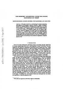
3 Geometric Properties of Shortest Paths This section summarizes the properties of shortest paths we use in our algorithm. Most of these de nitions and lemmas have appeared earlier [17, 18, 24]; we include them here for completeness. The triangle inequality implies that a Euclidean shortest path turns only at obstacle vertices. Shortest paths need not be unique, though|for instance, every obstacle polygon Oi has at least one point on its boundary reached by two shortest paths; the two shortest paths together form a cycle enclosing the polygon. We use the notation � (p; q ) to denote the set of shortest paths connecting two points p and q . The length of any path in � (p; q ) is the shortest path distance between p and q , denoted d(p; q ). (Clearly, if one or both points lie inside an obstacle, there is no legal path between them; their shortest path distance is assumed to be in nite.) If the shortest path between p and q is the line segment pq, then p and q are said to be mutually visible . We occasionally use d(X; Y ) to denote the shortest path distance between two sets of points X and Y , which is the minimum d(x; y ) over all pairs of points x 2 X and y 2 Y . We consider the problem of computing shortest paths from a xed point s to all points of the free space. We de ne the weight of an obstacle vertex to be its shortest path distance to s. Given an arbitrary point p in free space, its weighted distance to a visible vertex u is de ned as jpuj + d(u; s)|the straight-line distance from p to u plus the shortest path distance from u to s. Obviously, the shortest path distance d(p; s) is the minimum weighted distance between p and all vertices visible to p. The predecessor of an arbitrary point p is de ned as the vertex (or vertices) of V adjacent to p in � (p; s); recall that V includes both s and the obstacle vertices. A predecessor of p is necessarily visible from p. (If p and s are mutually visible, then s is a predecessor of p.) The shortest path map of a particular source point s, denoted SPM (s), is a subdivision of the plane into two-dimensional regions such that all the points in one region have the same, unique predecessor. Points on region boundaries have multiple predecessors. These boundaries are pieces of bisectors |a bisector is the locus of points equidistant (by weighted 12
distance) from two obstacle vertices, and it is in general an arc of a hyperbola. Figure 7 shows an example of a shortest path map.
s
Figure 7: SPM (s) and a wavefront sweeping it. The next three lemmas establish some fundamental properties of shortest paths and shortest path maps.
Lemma 3.1 The set of points in the plane with multiple predecessors has measure zero. Proof. A point p with two obstacle vertices u and v as predecessors lies on the
bisector of u and v , which is the hyperbola determined by the equation
jpuj + d(u; s) = jpvj + d(v; s): There are at most O(n2) such hyperbolas, and each has measure zero.
2
There are two types of edges in the subdivision SPM (s): (portions of) obstacle edges and arcs of hyperbolas determined by pairs of weighted vertices. The hyperbolic arcs may degenerate to straight lines|this happens when the weights of two vertices are equal, or di�er by precisely the distance between the vertices; in the latter case the vertex with smaller weight is a predecessor of the other vertex. The vertices of SPM (s) are of three types: the obstacle vertices, the intersections of obstacle edges with (bisector) hyperbolic arcs, and the intersections of two or more bisectors; each of the last variety of vertices has three or more predecessors. The following lemma proves a linear upper bound on the total size of a shortest path map.
Lemma 3.2 The shortest path map SPM (s) has O(n) vertices, edges, and faces. Each edge is a segment of a line or a hyperbola.
Proof. We rst observe that each face of SPM (s) is star-shaped, with the unique
predecessor vertex for the face in its kernel|this follows from Lemma 3.1, which shows that interior points of a face have a unique predecessor. The key step in the proof is to show that each obstacle vertex is the predecessor vertex for at most one face in SPM (s). Consider a vertex u that is the predecessor 13
of a face F , and let pred (u) be the set of predecessors of u; observe that d(u; s) = juvj + d(v; s), for any v 2 pred (u). By the triangle inequality, if a point p is visible from a vertex v 2 pred (u), with v; u; p not collinear, then p cannot have u as its predecessor. Let R(u; v) denote the region of the free space that is visible from u but not visible from v 2 pred (u). Then R(u; v) lies in an angular wedge around u of less than 180�. De ne \ R(u) = R(u; v): v2pred (u)
Clearly, F � R(u). We claim that there is at most one face of SPM (s) in R(u) with u as its predecessor. Suppose there were two faces, F1 and F2 , both having u as their unique predecessor. The faces F1 and F2 have exactly one point in common: the vertex u. In the space between F1 and F2 , there is a point p arbitrarily close to u with predecessor z such that z is distinct from both u and pred (u). In other words, jpuj + d(u; s) > jpz j + d(z; s). However, as p moves towards u, the di�erence in the distance shrinks, and nally d(u; s) = juzj + d(z; s). But then z must be a predecessor of u, contradicting the hypothesis. Thus, a vertex u is a predecessor of at most one face in the shortest path map. Finally, to prove the linear upper bound on the size of the shortest path map, recall that the number of obstacle vertices is n; the remaining vertices border at least three faces of SPM (s) (for this argument, we count the obstacle polygons as faces of the shortest path map). Since the number of faces is O(n), Euler's formula for planar graphs implies that the total number of vertices is also O(n). This completes the proof. 2 Lemma 3.3 Let u and v be two obstacle vertices that lie on the same side of a line `. If ` intersects the bisector generated by u and v more than once, the intersections lie on opposite sides of the line supporting uv . Proof. If the bisector is a straight line, the claim follows readily. Otherwise, the bisector is a hyperbola, and let us consider an arbitrary point p on this bisector. Every point on pu has u as its predecessor, and every point on pv has v as its predecessor. Points in the interiors of pu and pv have only one predecessor since they are not on the bisector. See Figure 8. If the half-bisector on one side of uv intersects ` at two points p and q , then there is an intersection of pu with qv or pv with qu that is not on the bisector and yet has two predecessors|a contradiction.
2
With these preliminaries in place, we can now describe our shortest path algorithm, which works by propagating a wavefront through the conforming subdivision of the free space.
4 The Shortest Path Algorithm Our algorithm uses the continuous Dijkstra method [18, 19, 20], which simulates a unit-speed wavefront expanding from a point source and spreading among the obstacles. At simulation 14
q
p
l u
v
Figure 8: The intersection of qu with pv has two predecessors, even though it is not on a bisector|a contradiction. time t, the wavefront consists of points whose shortest-path distance to the source is t. The wavefront is a set of disjoint paths and closed cycles. Each path or cycle is a sequence of circular arcs, called wavelets. Each wavelet is centered on an obstacle vertex that is already covered by the wavefront, called the generator of the wavelet. As the wavefront expands, the meeting point of two adjacent wavelets sweeps along a bisector curve, which is the hyperbolic bisector of the two wavelets' generators. The endpoints of paths in the wavefront are formed where wavelets meet obstacle boundaries; these endpoints sweep along obstacle boundaries as the wavefront expands. During the wavefront simulation, the topology of the wavefront is changed by events of two types: wavefront-wavefront collisions and wavefront-obstacle collisions. Our shortest path algorithm has two phases: a wavefront propagation phase, followed by a map computation phase. The rst phase simulates the wavefront and determines approximate locations of all the wavefront collision events. The second phase uses this information to build the shortest path map in each cell of the conforming subdivision. In the following two subsections, we describe the details of these two phases, deferring the data structures and implementation issues of the propagation until the next section.
4.1 The Propagation Algorithm
Our algorithm works by propagating the wavefront through the cells of the conforming subdivision of the free space. The wavefront propagates between adjacent cells only across transparent edges; it dies upon meeting an opaque edge. Propagating the exact wavefront appears to be quite di�cult, so we content ourselves with computing two \single-sided" approximations to the wavefront at each transparent edge. Speci cally, at each transparent edge, we compute two approximate wavefronts, passing through the edge in opposite directions. An approximate wavefront represents the wavefront reaching an edge from one side of the edge only. We can think of an approximate wavefront as labeling each point p on the edge with the time at which the approximate wavefront reaches p. The true distance d(p; s) is the minimum of the two labels from opposite sides of the edge.
Remark: In some cases we can determine that a portion of a wavefront arrives at an edge after
the wavefront from the other side of the same edge, and in such cases we drop the part that arrives later. In that sense, an approximate wavefront is not necessarily a complete representation of all the wavelets coming from one side of the edge.
An approximate wavefront at an edge e is represented as a sequence of obstacle vertices weighted with their shortest path distances from s. These vertices are the generators of 15
the wavelets in the approximate wavefront. All the generators in an approximate wavefront sequence lie on the same side of e, since the approximate wavefront passes through e in one direction only. The core of our algorithm is a method for computing an approximate wavefront at an edge e based on the approximate wavefronts of nearby edges. These nearby edges are formalized in the following with the de nitions of input (e) and output (e). We denote by input (e) the set of edges whose approximate wavefronts are used to compute the approximate wavefronts at e. This set consists of the transparent edges on the boundary of U (e), the well-covering region of e (cf. Section 2.1). To compute the approximate wavefront at e, we propagate the approximate wavefronts from input (e) to e inside U (e). The propagation algorithm introduces bends only at obstacle vertices in the closure of U (e); that is, the shortest paths corresponding to the wavefront do not bend except at obstacle vertices. Because U (e) need not be convex (nor even simply connected), nonconvexities of U (e) may block the wavefronts from some edges of input (e) from reaching e. Typically, the paths corresponding to blocked wavefronts either run into obstacles outside U (e), or they pass through free space outside U (e) and re-enter through other edges of input (e). We denote by output (e) the set of edges to which the approximate wavefronts of e will be passed; output (e) = input (e) [ ff j e 2 input (f )g. We set output (e) to contain input (e) because our algorithm for detecting wavefront collision events depends on output (e) having a cycle enclosing e.
Lemma 4.1 For any transparent edge e, output (e) contains a constant number of edges. Proof. Because jU (f )j = O(1) for all f , and each U (f ) is a connected set of cells of S 0 , no edge e can belong to input (f ) for more than O(1) edges f . 2 Our simulation of the wavefront propagation is loosely synchronized. For a transparent edge e = ab, we de ne d~(e; s) = min(d(a; s); d(b; s)); this is a rough estimate of d(e; s), since d(e; s) � d~(e; s) � d(e; s) + 12 jej. We compute the approximate wavefronts for e at the rst time we are sure that e has been completely covered by wavefronts from the edges in input (e). This time is d~(e; s) + jej, the approximate time at which the expanding wavefront rst hits an endpoint of e, plus the length of e. It is a conservative estimate of the time when e is completely run over by the wavefront. We compute d~(e; s)+ jej on the y for each edge e using a variable covertime (e). Initially, for every edge e whose well-covering region U (e) includes the source point s, we calculate an upper bound on d~(e; s) directly, considering only straight-line paths inside U (e), and set covertime (e) to this upper bound plus jej. For all other edges, we initialize covertime (e) = 1. Thus covertime (e) is not equal to d~(e; s) + jej only for edges e = ab such that �(a; s) or � (b; s) crosses the boundary of U (e). The simulation maintains a time parameter t, and processes edges in order of their covertime (�) values. The main loop of the simulation is as follows:
16
Propagation Algorithm
while there is an unprocessed transparent edge do 1. Select the edge e with minimum covertime (e), and set t := covertime (e). 2. Compute the approximate wavefronts at e based on the approximate wavefronts from all edges f 2 input (e) satisfying covertime (f ) < covertime (e). Compute d(v; s) exactly for each endpoint v of e. 3. For each edge g 2 output (e), compute the time tg when the approximate wavefront from e rst engulfs an endpoint of g . Set covertime (g ) := min (covertime (g ); tg + jg j).
endwhile
The following lemma proves the consistency of our algorithm|it shows that covertime () is correctly maintained and that the edges required for processing e are already processed. The details of Step 2 appear in Sections 4.1.1 and 4.1.2; the computation of tg in Step 3 is described in Section 5.
Lemma 4.2 During the wavefront propagation, the following invariants hold: (a) If the wavefront of an edge f 2 input (e) contributes to an approximate wavefront of e, then d~(f; s) + jf j < d~(e; s) + jej.
(b) The value of covertime (e) is updated a constant number of times. (c) The nal value of covertime (e) is d~(e; s) + jej. This value is reached no later than the simulation clock reaches that time. (d) Edge e is processed at simulation time d~(e; s) + jej. Proof.
(a) Any wavelet that contributes to the approximate wavefront at e must reach e at some time te with d(e; s) � te < d~(e; s) + jej. Such a wavelet reaches e either by traveling straight from s inside U (e), or by passing through a transparent edge f 2 input (e) at an earlier time tf , with d(f; s) � tf < d~(f; s) + jf j and te � tf + d(e; f ). By Condition (W3fs) of a well-covering region with parameter 2, d(e; f ) � 2jf j, and so te � d(f; s) + 2jf j. Since d~(f; s) � d(f; s) + 12 jf j, we can conclude that d~(f; s) + jf j < d~(e; s) + jej. (b) The value of covertime (e) is updated only when an edge f is processed such that f 2 input (e) or e 2 input (f ). There are O(1) such edges, by Lemma 4.1. of well-covering. (c); (d) We prove these by induction on the simulation clock. Claims (c) and (d) hold for the edges whose initial covertime (�) values are not in nite. The wavelet that rst 17
reaches an endpoint of e (at te = d~(e; s)) passes through some f 2 input (e). By induction and the proof of (a), f has already been processed before the simulation clock reaches te , and so covertime (e) is set to d~(e; s) + jej no later than te = d~(e; s). The variable covertime (e) cannot be set to any smaller value, because no approximate wavefront can reach the endpoints of e earlier than d~(e; s). It follows that e will be processed at simulation time d~(e; s) + jej. 2
Lemma 4.3 For every vertex v of our conforming subdivision, the propagation algorithm correctly determines the distance d(v; s) before v is used as a generator in any wavefront. Proof. Every vertex v of the conforming subdivision is an endpoint of a transparent
edge e. The wavefront that determines d(v; s) either reaches v from s by traveling only inside U (e), or it passes through an edge f 2 input (e) such that covertime (f ) < covertime (e). In the former case, initialization computes d(v; s) correctly; in the latter case, Step 2 of the propagation algorithm implies that d(v; s) is correctly computed. If v is an obstacle vertex, it may appear as a generator in a wavefront, but it will not be used until after d(v; s) is computed at time d~(e; s)+ jej (Lemma 4.2(d)).
2
While a well-covering region U (e) has constant complexity, it is not necessarily simplyconnected; consider, for instance, the case of a square annulus. Consequently, there may be multiple, topologically distinct paths from a boundary edge f 2 input (e) to e. In order to avoid comparing paths of di�erent topologies, we split the wavefront W (e) into topologically-equivalent pieces. In particular, let W (e) denote one of the two approximate wavefronts passing through e. In computing W (e) from a set fW (f ) j f 2 input (e)g, we use topologically constrained versions of the incoming wavefronts, denoted W (f; e). A wavefront W (f; e) is a portion of W (f ) that follows a single topological path inside U (e) from f to e. If U (e) contains islands, there are multiple topologically distinct paths from an edge f 2 input (e) to e. When we need to refer to multiple topologically distinguished wavefronts from a single edge f to e, we use primed notation: W (f; e), W (f 0; e), etc. If two points p; q 2 e are hit by a single topologically constrained wavefront W (f; e), then the segments connecting p and q to their predecessors among the generator vertices in W (f ) intersect f and e, and the quadrilateral bounded by those segments and f and e is a subset of U (e). (The paths are not always segments: if an obstacle vertex v lies in the well-covering region of e and the path from f to p turns at v , then the predecessor of p in W (f; e) may be v . Even in this case, the paths from p and q to f can be continuously deformed to each other inside U (e).) For any point p 2 e, the shortest path � (p; s) passes through some f 2 input (e) (unless s 2 U (e)), so constraining the source wavefronts to pass through input (e) does not lose any essential information.
4.1.1 The Arti cial Wavefronts
When we compute the approximate wavefronts at a transparent edge e, we allow limited interaction between waves coming from opposite sides of the edge. This lets us eliminate some waves coming from one side of the edge that are dominated by waves from the other side. The interaction between the wavefronts from two sides is implemented using arti cial 18
wavefronts . These arti cial wavefronts are our only mechanism for pruning the wavefront that arrives second at a transparent edge. We depend on arti cial wavefronts to eliminate dominated wavefronts within a constant number of cells of where they rst become dominated. Consider a horizontal transparent edge e, and let v be an endpoint of e. We introduce an arti cial wavefront with generator v and weight d(v; s) into the computation of both approximate wavefronts at e. The triangle inequality implies that d(p; s) � d(v; s) + jvpj, for any point p 2 e. If the arti cial wavefront reaches p 2 e before the wavefront from below e reaches p, then p is surely reached rst by the upper wavefront, and so there is no need to propagate the lower wavefront through p. See Figure 9 for an illustration. In essence, an arti cial wavefront is a convenient mechanism for discarding parts of the actual wavefront that are completely dominated by some other part of the wavefront. A generator of an arti cial wavefront is not passed on to output (e) as part of the approximate wavefront, unless it is also a vertex of O. Remark: An arti cial wavefront is just a conceptual device that lets us argue about shortest paths without having to exhibit a speci c shortest path. We use this technique in our proofs (e.g. Lemma 4.8) to discard generators at a cell boundary if the wavelet from an arti cial wavefront reaches that boundary before the wavelets from those generators|since the path passing through an arti cial generator is no shorter than the true path from the predecessor of the arti cial generator, the paths from the losing generators cannot be shortest paths. from s p v
Figure 9: An arti cial wavefront generated by v . If d(v; s) + jvpj is less than the time at which the wavefront from below reaches p, then p is reached rst by a wavefront from above. When we compute the approximate wavefront passing through e from below (that is, coming from predecessors below e), the contributing wavefronts are the following: 1. All wavefronts W (f; e) for f 2 input (e) and f below the line supporting e. (If f intersects the line supporting e, we split W (f; e) in two, and keep only the portion W (f 0; e) that comes from the part of f below e.) 2. An arti cial wavefront expanding from each endpoint of e. An arti cial wavefront generator v has weight d(v; s). The contributing wavefronts for the approximate wavefront passing through e from above are symmetric. The wavefront coming directly from s is handled separately. The approximate wavefront from below is what the true wavefront would be if we were to block o� the wavefront from above by adding extra obstacles. In physical terms, we 19
can imagine replacing the transparent edge e with an (open) opaque obstacle segment. The opaque segment absorbs the wavefront from above, but the open endpoints let the wavefront from above pass through to generate arti cial wavefronts. (Open endpoints are needed only to guard against the case in which an actual obstacle segment shares an endpoint of e, in which case replacing e with a closed segment would prevent arti cial wavefronts from passing through the endpoint.) Consider a set of wavefronts that reach e from the same side. We say that a contributing wavefront W (f ) claims a point p 2 e if W (f ) reaches p before any other contributor from the same side of e.
Lemma 4.4 Let e be horizontal, and let W (f; e) and W (g; e) be two contributors to the
approximate wavefront that passes through e from below. Let x and x0 be points on e claimed by W (f; e), and let y be a point on e claimed by W (g; e). Then y cannot lie between x and x0 . Proof. Consider the shortest paths � (x; s), � (x0; s), and � (y; s) in the modi ed
environment in which e has been replaced by an open, opaque segment. These paths connect x and x0 to f , and y to g , inside U (e). Shortest paths � (x; s), � (x0; s), and � (y; s) do not cross. The subpaths of � (x; s) and � (x0; s) inside U (e) can be continuously deformed to each other inside U (e), so g is not between them. It follows that y is not between them, either. 2
Lemma 4.5 Let u and v be two obstacle vertices, both generating wavelets that are con-
sidered when the approximate wavefront passing through an edge e from below is computed. Then the bisector generated by u and v intersects e at most once in SPM (s). Proof. Suppose the bisector intersects e twice. Without loss of generality assume u lies inside the loop formed by the bisector and e. If the bisector intersects e twice in SPM (s), then the segment from u to its predecessor must intersect e between the two bisector intersections. This means that d(e; s) < d(u; s); in fact, d(e; s) + 2jej � d(u; s). Hence d~(e; s) + jej < d(u; s), and u cannot contribute to the approximate wavefront at e: it does not become a generator until after e is processed, contradicting the assumption that both u and v contribute to the approximate wavefront at e. 2
Lemma 4.6 Given W (f; e) for each f below e that contributes to W (e), we can compute
the interval of e claimed by each W (f; e) in O(1+ k) total time, where k is the total number of generators in all wavefronts W (f; e) that are absent from W (e). Proof. For each contributing wavefront W (f; e), we show how to determine the
portion of e claimed by W (f; e) if only one other contributing wavefront W (g; e) is present. Lemma 4.4 implies that this portion is contiguous. The intersection of these claimed portions, taken over all other contributors W (g; e), is the part of e claimed by W (f; e) in W (e). In constant time we determine whether the claim of W (f; e) is left or right of that of W (g; e). If both W (f; e) and W (g; e) reach the left endpoint of e, in constant time check which one reaches it sooner. Otherwise, one of W (f; e) and W (g; e) reaches a point on e that is left of any point reached by the other, and this point determines 20
pa
pb x
a
e
b
Figure 10: The contribution of b to W (e) is constrained to be left of pb and right of x, and therefore does not exist. the ordering. Without loss of generality, assume that the claim of W (f; e) is left of that of W (g; e). By Lemma 4.4, we can combine the two wavefronts using only local operations. Let a denote the generator in W (f; e) claiming the rightmost point on e. Let pa be the left endpoint of a's interval on e. Similarly, let b denote the generator in W (g; e) claiming the leftmost point on e, and let pb be the right endpoint of b's interval on e. Compute the bisector of a and b, and let its intersection with e be the point x. (By Lemma 4.5, there is only one intersection point in SPM (s). If the hyperbola generated by a and b intersects e twice, then a is to the left of b at only one of the intersections, and we use that intersection as x.) See Figure 10. If x is to the left of pa , then delete a from W (f; e); if x is to the right of pb , then delete b from W (g; e); in either case, rede ne a, b, pa , pb , recompute x, and repeat this test. If pa is left of pb and x lies between them, then x is the right endpoint of W (f; e)'s claim in the presence of W (g; e). By combining the claimed regions for all contributors W (f; e), we construct the approximate wavefront at e. The time bound follows since we spend constant time per generator that is deleted for each pair of wavefronts, and the total number of wavefronts W (f; e) to be merged is also a constant. This nishes the proof. 2
Lemma 4.7 Any generator deleted during the construction of an approximate wavefront at
edge e does not contribute to the true wavefront at e. Every generator that contributes to the true wavefront at e either is s or belongs to one of the approximate wavefronts at e. Proof. The rst part is clear|every deleted generator is dominated by some other generator at e. The second part follows by induction from two facts: any wavelet that contributes to the true wavefront at e must come either from s inside U (e) or through one of the edges in input (e) (by the de nition of well-covering). The approximate wavefronts at input (e) are ready before they are needed to construct W (e) (by Lemma 4.2). 2
21
4.1.2 The Bisector Events
When we propagate an approximate wavefront W (e) to output (e), we may detect bisector events, which are intersections of bisectors with each other or with obstacles. Bisector events are detected in two ways: 1) during the computation of W (e; g ) from W (e) for some g 2 output (e); 2) during the merging process described in Lemma 4.6. 1. Bisector events of the rst kind are detected when we simulate the advance of the wavefront from e to g to compute W (e; g ); the details of this simulation are discussed in Section 5. In particular, if two generators u and v are non-adjacent in W (e) but become adjacent at any time during the propagation from e to g , then there is a bisector event involving u and v . 2. Bisector events of the second kind are detected during merging. If a generator v contributes to one of the input wavefronts W (e; g ) but not to the merged wavefront W (g) at g, then v is involved in a bisector event on the way from e to g. (As a special case, if a generator's claim on W (g ) is shortened (but not eliminated) by an arti cial wavefront, then that generator is also considered to have a bisector event. This adds at most two extra bisector events for each edge g .) Our algorithm detects bisector events in a small neighborhood of their actual location in SPM (s). To ensure that all bisector events are properly localized, we mark the generators that participate in a bisector event in O(1) cells near where the event is detected: if a generator v is involved in a bisector event in a cell c, then v is guaranteed to belong to a set of marked generators for c. However, the set of marked generators for a cell c may be a superset of the generators that actually participate in bisector events in c. We will show that the total number of generators marked in all the cells is O(n). The precise rules for marking the generators are given below.
22
Marking Rules for Generators
1. If a generator v lies in a cell c, then mark v in c. 2. Let e be a transparent edge, and let W (e) be the approximate wavefront coming from some generator v 's side of e. (a) If v claims an endpoint of e in W (e), or if it would do so except for an arti cial wavefront, then mark v in all cells incident to the claimed endpoint. (b) If v 's claim in W (e) is shortened or eliminated by an arti cial wavefront, then mark v in the cell on v 's side of e. 3. Let e and f be two transparent edges with f 2 output(e). Mark v in both the cells that have e as an edge if one of the following events occurs: (a) v claims an endpoint of f in W (e; f ); (b) v participates in a bisector event detected either during the computation of W (e; f ) from W (e), or during the merging step at f (Lemma 4.6). (We also mark v as having a bisector event if v 's claim on W (f ) is shortened by an arti cial wavefront.) 4. If v claims part of an opaque edge when it is propagated from an edge e toward output (e), mark v in both cells with e on their boundary. Rules 2a and 3a both apply when a wavefront claims an endpoint of an edge. The main di�erence between the two rules is that Rule 2a puts marks in cells near the claimed endpoint, and Rule 3a puts marks in cells near the source edge of the wavefront. A generator may contribute to a wavefront more than once in the wavefront sequence; each mark applies to only one instance of the generator in the sequence. The following technical lemma is used in the proof of Lemma 4.9 to establish the correctness of the marking rules.
Lemma 4.8 Let v be a generator that contributes to an approximate wavefront W (e). Suppose there is a point p 2 e that is claimed by v in W (e) but not in SPM (s) (because a wave from the other side of e reaches p rst). Then v is marked in the cell c on v 's side of e. Proof. If v is unmarked in c, there must be generators u and w such that u; v; w
are consecutive in W (e)|otherwise Rule 2 would apply. The bisectors (u; v ) and (v; w) must exit from U (e) through the same transparent edge h|otherwise Rule 3 or 4 would apply. For the same reason, the region bounded by (u; v ), (v; w), h, and e is a subset of of U (e)|if the region contained a non-U (e) island, v would claim an endpoint of a boundary edge of that island. Edge h is by de nition part of input (e). Consider the point p 2 e that is claimed by v in the approximate wavefront W (e) 23
but not in the true wavefront at e, and suppose that the true predecessor of p is z 6= v. The vertex z is either an obstacle vertex or the source s. In the former case, z lies outside U (e) or on its boundary @ U (e)|by Condition (C3), U (e) contains at most one obstacle vertex, so any vertex not strictly outside U (e) must be connected to points outside U (e) by opaque edges. Vertex z may lie strictly inside U (e) only if z = s. Let us rst assume that z lies outside the well-covering region U (e)|the proof simpli es in the other case, which is considered below. Let q denote the intersection point between zp and input (e) closest to p (recall that input (e) � output (e), and input (e) � @ U (e)). Based on the position of q relative to the bisectors (u; v ) and (v; w), we argue that v must have been involved in a bisector event detected by our algorithm, and thus marked in cell c. First, consider the case in which q lies between the bisectors (u; v ) and (v; w) on the edge h. Now, since jqpj � jhj (by the well-covering property), the endpoints of h are engulfed by a wavefront from z or from some other generator before the wavefront from z reaches p at time d(z; s) + jzpj. The arti cial wavefronts from h's endpoints will cover h before time d(z; s) + jzpj + jhj. By assumption we have d(v; s) + jvpj > d(z; s) + jzpj. The wavefront from v cannot reach e earlier than d(v; s)+jvpj?jej. By well-covering with parameter 2, d(e; h) is at least jej+jhj, and so the wavefront from v reaches h no earlier than d(v; s)+ jvpj + jhj > d(z; s)+ jzpj + jhj, at which time h is already covered by the arti cial wavefront. The claim of v on h is shortened by the arti cial wavefront (in fact, v 's claim is eliminated completely), and so it must be marked by Rule 3b. In the second case, q is not between the bisectors (u; v ) and (v; w) on h. The segment qp must intersect one of the bisectors. Without loss of generality, assume qp intersects bisector (u; v). Since every point on qp has z as its predecessor in SPM (s), the bisector (u; v ) does not reach @ U (e) in SPM (s). We show that our propagation and merging algorithms will detect a bisector event for (u; v ). Let r be the intersection point between the bisector (u; v ) and the edge h. As noted in the discussion after Lemma 4.3, the triangle de ned by the segments ur, vr, and e is a subset of U (e). Bisector (u; v ) crosses the triangle boundary on e and at r, but nowhere else. The larger region R bounded by e, h, ur, and bisector (v; w) also is a subset of U (e), and it contains point p. Because qp crosses into R to intersect (u; v ), and it does not intersect the (v; w) or h sides of R, qp must intersect ur; let x be the point of intersection. The wavelet from z reaches x before the one from u, so the path z ! x ! r, starting at time d(z; s), reaches r before the path u ! r, starting at time d(u; s). Observe also that the path z ! x ! r is a legal path|it lies in free space. Now, consider the shortest path from z to r inside the triangle 4zxr that does not cross h or any obstacle edge (see Figure 11). Because z ! x ! r lies in free space, such a path exists, and is shorter than z ! x ! r. This path claims r from the same side as u before the wavelet from u reaches r. (If the path passes through an endpoint of h, then an arti cial wavefront claims r; otherwise the last obstacle vertex on the path claims r.) Thus, a bisector event for (u; v ) is detected during the computation of W (e; h) or W (h), and v is marked by Rule 3b. 24
z q
r h x e
p u
v
w
Figure 11: The shaded path from z to r claims r before the wavelet from u, and from the same side of h as u. Next consider what happens if the predecessor vertex z lies on the boundary of the well-covering region U (e). Let h be a boundary edge of U (e) incident to z . In this case we detect a bisector event involving v when we advance the wavefront from e to output (e): if z lies between the bisectors (u; v) and (v; w), then v is marked by Rule 3a or 4; if z is not between the bisectors, the segment zp intersects one of the bisectors, say (u; v ), and we detect a bisector event for (u; v ) in advancing the wavefront from e to output (e). Finally, consider the case in which z = s lies inside U (e). If z is not between the bisectors (u; v ) and (v; w), segment zp intersects one of them and the proof is as above. Let r be the intersection of (u; v ) with h, and let t be the intersection of (v; w) with h. The convex quadrilateral bounded by subsegments of e, ur, h, and tw is contained inside U (e). Hence if z is between the bisectors (u; v) and (v; w), the entire segment rt is visible from z (that is, 4zrt is empty) and so v 's claim on h is eliminated by z . Therefore v is marked by Rule 3b. This completes the proof. 2
Lemma 4.9 If a generator v participates in a bisector event of SPM (s) in a cell c, then v
is marked in c.
Proof. If a bisector has an endpoint on an opaque edge of c, it either emanates from
an obstacle vertex on the edge, or it is de ned by two generators that claim part of the opaque edge. Rules 1 and 4 guarantee that all such generators are marked in c. If a generator v that contributes to an approximate wavefront in c is unmarked, then by Rule 2a there must be transparent edges e and f on the boundary of c such that W (e) and W (f ) both contain the generator subsequence u; v; w, for some u and w. Without loss of generality assume W (e) enters c and W (f ) leaves c. If v participates in a bisector event of SPM (s) in c, then at least one point p inside the region R bounded by e, f , (u; v ), and (v; w) is not claimed by v in SPM (s). Let z be the true predecessor of p. Let r and t be the intersections of (u; v ) and (v; w) with f , respectively. Region R is contained in the convex quadrilateral Q bounded by ur, rt, tw, and the line supporting e. Because u; v; w is a subsequence of W (e), no vertex 25
on the same side of e as v claims any point of the side of Q collinear with e; that is, zp does not cross that side of Q. If r and t are both claimed by v in SPM (s), then ur 2 � (s; r), and wt 2 � (s; t). In this case � (s; p) cannot cross ur or wt, and hence it must cross rt. The intersection of zp with rt is a point q that satis es the hypothesis of Lemma 4.8, and so v is marked in c. On the other hand, if either r or t is not claimed by v in SPM (s), that vertex satis es the hypothesis of Lemma 4.8, and so v is marked in c. 2 The following technical lemma shows that the approximate wavefronts are not too di�erent from the true wavefronts; this lets us bound the number of marks made by the marking rules.
Lemma 4.10 Let B be the set of pairs (e; b) of transparent edges e and bisectors b such
that b crosses e in some approximate wavefront, but the same crossing does not occur in SPM (s). Then jB j = O(n). Proof. Let (e; b) be a pair in B . Bisector b is de ned by two generators u and v .
The proof of Lemma 4.8 notes that each generator (except possibly s) is outside or on the boundary of U (e). That proof also shows that b's intersection with e in some approximate wavefront (that is, the presence of u and v in W (e)) is proof that u and v claim points on the boundary of U (e) (in input (e)) in SPM (s). Let p = b \ e. Because (e; b) is not an incident pair in SPM (s), there must be at least one bisector event in SPM (s) that lies in the interior of U (e) between the line segments up and vp. We can charge the early demise of b to any one of these bisector events. The segments pu and pv are disjoint inside U (e) from the corresponding segments de ned by any other pair (e; b0) 2 B |in the modi ed shortest path problem in which the obstacles are O [ feg, the segments pv and pu belong to � (s; p), and hence they * and * are disjoint from any other such segments. Thus the sector bounded by pu pv 0 is disjoint inside U (e) from the sector de ned by any other pair (e; b ) 2 B , so each bisector event inside U (e) is charged at most once for all pairs in B that have e as the rst element of the pair. Each cell in the conforming subdivision belongs to O(1) well-covering regions U (e). Hence the sum over all transparent edges e of the number of bisector events in U (e) is only O(n). This total is an upper bound on jB j.
2
Lemma 4.11 The total number of marked generators over all cells is O(n). Proof. We begin by de ning a propagation region for each edge e. For any
transparent edge e, let P (e) be the collection of cells through which wavefronts propagate on the way from e to all edges f 2 output (e). Clearly P (e) � U (e) [ fU (f ) j f 2 output (e)g. The number of cells in P (e) is constant, since joutput (e)j is constant, and so is the number of cells in U (f ) for any f . Furthermore, since every cell of P (e) is within a constant number of cells of e, each cell c belongs to P (e0 ) for only a constant number of edges e0 . The total number of generator-cell marks made under Rule 1 is clearly O(n). 26
Each P (e) has constant complexity, so there are O(n) edge pairs (e; f ), where e is transparent and f is either transparent and in output (e), or opaque and inside or on the boundary of P (e). From this it follows that the number of marks made by Rules 2a and 3a is O(n). Similarly, there are O(n) Rule 4 marks in which the wavelet from v claims an endpoint of the opaque edge, or is the rst or last non-arti cial wavelet in W (e). Any Rule 4 mark not yet counted involves a generator v that does not reach any opaque edge endpoint when propagated forward from e. Because v is not the rst or last non-arti cial wavelet in W (e), there is a generator u such that v 's claim on e in W (e) is bounded on the left by bisector (u; v). We can assume that (u; v) intersects e in SPM (s); by Lemma 4.10 there are only O(n) bisector-edge pairs that intersect in approximate wavefronts but not in SPM (s). Bisector (u; v ) terminates in P (e), either on the opaque edge or in a bisector event before the opaque edge. Let us charge the marking of v at e to this endpoint of (u; v ) in SPM (s). Because each cell belongs to P (e0 ) for a constant number of edges e0 , each vertex of SPM (s) is charged O(1) times. Since jSPM (s)j = O(n), the number of Rule 4 marks is O(n). The proofs for Rules 2b and 3b are similar to that for Rule 4. We begin with the proof for Rule 3b. We can assume that the interval claimed by v on e in W (e) is bounded by two bisectors (u; v ) and (v; w), for two non-arti cial generators u and w; the rst and last generators in W (e), counted separately, sum to at most O(n) overall. Furthermore, we can assume that (u; v) and (v; w) both intersect e in SPM (s); there are only O(n) bisector-edge pairs that appear in some approximate wavefront but not in SPM (s) (Lemma 4.10). At least one of the two bisectors fails to reach the boundary of P (e) in SPM (s), because Rule 3b applies, and a detected bisector event implies the existence of an actual bisector event no later than the point of detection; we charge the marking of v to that bisector endpoint. Each bisector event gets charged O(1) times, and there are O(n) bisector events in SPM (s). To bound the number of Rule 2b marks, consider where the generator v lies. There is at most one generator v inside U (e), and so O(n) marks for such generators overall. If v lies outside U (e), there is at least one edge in input (e) where v is marked by Rule 3b because of the shortening of v 's claim on e. Charge the Rule 2b mark at e to this Rule 3b mark. There are O(n) Rule 3b marks and hence O(n) Rule 2b marks. 2 We defer the ner details of the propagation algorithm to Section 5, and instead describe the second phase of the algorithm next, namely, the shortest path map computation.
4.2 Computing the Shortest Path Map
At the end of the propagation phase, approximate wavefronts for all transparent edges have been computed. Furthermore, for every cell c, a set of marked generators is known; each marked generator is in the approximate wavefront of one of the boundary edges of c, and all but O(1) of them contribute to a bisector event either in c or in one of O(1) nearby cells. The algorithms of Lemma 4.6 and Section 5 let us compute the marked generators in O(log n) time apiece. 27
We now show how to break the interior of a cell c into active and inactive regions such that no vertices of SPM (s) lie in the inactive regions. By Lemma 4.9, no unmarked generator contributes to a bisector event in c. A bisector de ned by a marked generator and an unmarked neighbor belongs to SPM (s). All such bisectors are disjoint. They partition c into regions such that each region is claimed only by marked generators or only by unmarked generators. These are the active and inactive regions, respectively. See Figure 12. The active regions can be computed in time proportional to the number of marked generators in c, since the order of the generators along the boundary of c is known. A
I A
A I
I A A A
I
A
Figure 12: Active regions (white) and inactive regions (shaded). Each region-bounding bisector is de ned by one marked and one unmarked generator. The boundary of an active region consists of O(1) segments. Each segment is a transparent edge fragment, an opaque edge, or a bisector in SPM (s). Let e be a transparent edge fragment bounding an active region, and let W (e) be the wavefront that enters the active region by crossing e. In the absence of wavefronts from other transparent edges, W (e) partitions the active region into pieces we call S -faces, each with a unique predecessor in W (e). These S -faces may not cover the active region, since each point in an S -face must be connected to its predecessor by a segment that intersects e. Denote this partition by S (e). S (e) is essentially a shortest path map, restricted to the active region and considering only generators in W (e). If a point p lies in an S -face of S (e) with predecessor v , then S (e) assigns weight jpvj + d(v; s) to p. Points outside any S -face are assigned in nite weight by S (e). We can compute S (e) in O(m log m) time, where m = jW (e)j, by using the propagation algorithm and data structure of Section 5. The following lemma shows how to combine the wavefronts incident to di�erent boundary edges of an active region.
Lemma 4.12 Given the approximate wavefronts on the boundary of a cell c and a set of k marked generators in those wavefronts, we can compute the vertices of SPM (s) inside c in time O(k log k). Proof. Consider an active region inside c and two transparent edge fragments e and
f on the boundary of this active region. We can use the merge step from a standard divide-and-conquer Voronoi diagram algorithm to compute the portion of the region 28
nearer to W (e) than to W (f ), using weighted distance, in time O(jW (e)j + jW (f )j). More speci cally, assume that S (e) and S (f ) have both been computed. Let m = jW (e)j + jW (f )j. Each of S (e) and S (f ) de nes a distance function on the points of the active region. The point-wise minimum of these two functions determines which points are nearer to W (e) than to W (f ) under weighted distance. Consider a point p in the S -face for some generator v 2 W (e). Point p belongs to v 's S -face in SPM (s) only if all of the segment pv is closer to v than to any generator in W (f ). The set of points p such that the entire segment from p to its predecessor is closer to W (e) than to W (f ) is bounded by a single chain ? of O(m) hyperbolic arcs. (The number of arcs follows from Lemma 3.2.) To nd ?, rst trace along a ray emanating from some generator v 2 W (e), marching through S (e) and S (f ) simultaneously, until the ray reaches the boundary of c or reaches a point whose weight in S (f ) equals its weight in S (e). This takes O(m) time, since a line cuts O(m) edges of S (e) and S (f ). Then trace outward from this point along ?. Each arc of ? is a hyperbola determined by the generators of the S -faces of S (e) and S (f ) containing the current point; trace along the hyperbola until it leaves one of the two S -faces, then follow the hyperbola determined by the next pair of S -faces, etc. This procedure takes O(1) time per arc of ?, or O(m) time altogether. See Figure 13.
v f e
Figure 13: To nd the region closer to W (e) than to W (f ) under weighted distance, trace a ray from some v 2 W (e) through S (e) and S (f ) until it hits a point equidistant from the two wavefronts, then trace outward from the point along the bisector ?. The tracing procedure computes the region closer to W (e) than to W (f ) for one edge f . Intersecting the results for all such edges f on the boundary of the active region produces the region R(e) claimed by W (e) in SPM (s). Intersecting R(e) with S (e) gives the vertices of SPM (s) to which W (e) contributes. We repeat this computation for each transparent edge fragment to nd all the vertices of SPM (s) in the active region. Applying this algorithm to all active regions nds all vertices of SPM (s) inside c. The partition S (e) determined by each edge fragment e participates O(1) times in a Voronoi-style merge, so the total cost of merging is O(k). Hence the running time is dominated by the propagation algorithm, which takes O(k log k) time altogether.
2
29
Lemma 4.13 The shortest path map vertices computed cell-by-cell can be combined to build
SPM (s) in additional O(n log n) time. Proof. To compute SPM (s), we compute all its edges separately, then use a standard plane sweep to assemble them, as follows. Create a list of the bisector endpoints discovered in the computation of Lemma 4.12, each identi ed by a key consisting of two generators. Put each three-bisector endpoint into the list three times, once for each bisector. Put each bisector/edge collision in once, labeled with the generators of the bisector. Now sort the list to group together endpoints belonging to each bisector. Take the endpoints belonging to the bisector of a generator pair (v; w) and sort them along the hyperbola determined by the weighted generators v and w. This determines all edges of SPM (s) on the hyperbola. Doing this for all pairs that appear as keys in the sorted list gives all O(n) hyperbolic arcs of SPM (s). Finally, with a standard plane sweep [23], we can combine these arcs with the edges of O to build the subdivision SPM (s). 2
5 An Implementation of the Wavefront Propagation In this section, we give the implementation details of our algorithm. We describe the data structures used by our algorithm, and ner details of the propagation algorithm.
5.1 The Data Structures
An approximate wavefront is a list of generators (obstacle vertices). Our algorithm performs the following two types of operations on these lists: 1. Standard list operations: insert, delete, concatenate, split, nd previous and next elements, and search. The search operation locates the position of a query point in the list of bisectors de ned by the generators at a particular time. 2. Priority queue operations: we assign each generator in the list a priority, and the data structure needs to update priorities and nd the minimum priority in the list. Both of these types of operations can be supported by a data structure based on balanced binary trees, for example red-black trees, with the generators at the leaves. In particular, the list operations take O(log n) time each because the maximum list length is O(n). The priority queue operations are supported by adding a priority eld to the nodes of the binary tree: each node records the minimum priority of the leaves in its subtree. Each priority queue operation takes O(log n) time, while the list operations retain their O(log n) bound. We also require our data structure to be fully persistent|we need the ability to operate on past versions of any list. Each of the two kinds of operations uses O(1) storage per node of the binary tree, so we can make the data structure fully persistent by path-copying. Each of our operations a�ects O(log n) nodes of the tree, including all the ancestors of every a�ected node. Once we have determined which nodes an operation will a�ect, and before the operation modi es any node, we copy all of the nodes that will be a�ected, then modify the copies. This creates a new version of the tree while leaving the old version unchanged. The data structure uses O(m log n) storage, where m is the total number of data structure operations, and keeps the O(log n) per-operation time bound quoted above. 30
Lemma 5.1 There is a linear-space data structure that represents an approximate wave-
front and supports list operations and priority queue operations in O(log n) time per operation. The data structure can be made fully persistent at the expense of an additional O(log n) space per operation.
5.2 Details of the Wavefront Propagation
Using the data structures just described, we now show how to propagate an approximate wavefront from edge to edge. In particular, given an approximate wavefront W (e), we show how to compute W (e; g ) for every edge g 2 output (e). In the process, we also determine the time of rst contact between W (e; g ) and the endpoints of g . We describe how to compute W (e; g ) for all the transparent edges g on the boundary of e's cell. Because the edges of output (e) belong to a constant number of cells in the neighborhood of e, we can use this primitive to compute W (e; g ) for all g 2 output (e). When we propagate the wavefront cell-by-cell, we e�ectively split W (e; g ) into multiple pieces, each labeled by the sequence of transparent edges it follows from e to g . We assemble W (e; g ) out of these component wavefronts by concatenating pieces that correspond to topologically equivalent paths inside U (e). (Recall that for a pair e and g , there may be several constrained wavefronts W (e; g ), W (e0; g ), etc., topologically distinguished by the paths they follow among the islands inside U (e).) Each component piece is a list of generators; adjacent pieces may contain a single duplicate generator, namely the generator that claims the common endpoint. Before concatenation of the lists, one copy of the duplicate generator is deleted. In Figure 14, W (e; g ) is assembled from W (e0 ; g ) and W (e00; g ), where e0 and e00 are two edges on the boundary of g 's cell. g e' e" e
Figure 14: W (e; g ) may reach g via multiple paths.
5.2.1 Preparing the Cells for Propagation
The propagation algorithm that follows assumes that the cell c is convex. When c is nonconvex, which is the case for subcells of an annulus cell, we temporarily break c into convex subcells by adding transparent edges parallel to e through the points of nonconvexity, as illustrated by Figure 15. Let f 6= e be another transparent edge on the boundary of c. Our propagation algorithm assumes the following invariant: 31
obstacle
e
e
Figure 15: Preparing nonconvex cells for wave propagation.
Propagation Invariant: When a wavefront W (e; f ) is propagated for distance 2jf j beyond f , it intersects only a constant number of cells of the conforming
subdivision of the free space.
The edges of the conforming subdivision S 0 already satisfy the Propagation Invariant, since each edge f is well-covered with parameter 2. However, we need to be more careful in dealing with a cell derived from an annulus. We subdivide each of the newly added, nonconvexity-removing edges into O(1) pieces, each no longer than the edges of S on the annulus's outer boundary (one-eighth the side length of the outer square, by the uniform edge property of the conforming subdivision). Let H denote the convex hull of e and the inner square of the annulus. If H intersects a newly added edge f , then we further partition f \ H into pieces no longer than the inner boundary's edges (one-eighth the side length of the inner square). We illustrate this last step in Figure 16. Because f is parallel to e, and the inner boundary of the annulus is well separated from the outer boundary (cf. the minimum clearance property of the conforming subdivision S ), the total length of edges inside H is proportional to the side length of the inner square. It follows that the partition step creates only O(1) edges. The subdivided edges satisfy the Propagation Invariant: for any such edge f , let g 0 be an edge of c such that W (e; f ) leaves c by passing through g 0. Edge g 0 is an edge of S 0, the conforming subdivision of free space; it is a fragment of an edge g of S , the conforming subdivision for the vertices. The construction of S 0 in Lemma 2.2 ensures that there are O(1) cells of S 0 within shortest path distance 2jgj of g 0. The subdivision of nonconvexityremoving edges guarantees that jf j � jg j, which implies that the Propagation Invariant holds for edge f .
5.2.2 Simulating the Wavefront Propagation Across Convex Cells So far we have used a wavefront in its static form, namely, as a sequence of generators whose bisectors intersect an edge in the subdivision. We now describe a dynamic form of the wavefront, in which we track changes in the combinatorial structure of the wavefront as it sweeps across a cell. In particular, we simulate the evolution of a wavefront W (e) as it sweeps across a cell c after entering it through the edge e; the cell c is a convex cell satisfying the Propagation Invariant. Our simulation detects and processes any bisector events involving the generators of W (e) that may occur inside c. Events are processed in 32
f H e
Figure 16: Subdividing the added edges. order of increasing distance from s, that is, in simulation time order. Generators are marked as events are processed, though the description below does not necessarily itemize all the marks made. Let W denote the current dynamic wavefront at any time during the simulation. At the start of the simulation, we have W = W (e), the approximate wavefront that passes through e|it is a list of generators, each claiming some portion of e. Every generator v 2 W de nes a pair of bisectors with its neighbors in the list. If v is the rst generator in the list, then its rst bisector is the ray from v through the endpoint of e at v 's end of the list; the last bisector for the last generator is de ned similarly. If v is an endpoint of e, then there is no rst bisector (or last bisector, as appropriate). To process bisector events in order, we maintain the corresponding generators of W in a priority queue. The priority of a generator v is the weighted distance to the point at which the two bisectors de ned by v intersect beyond e; the priority is in nite if the bisectors do not intersect beyond e. Speci cally, if the bisectors de ned by v and its neighbors intersect ahead of e, either in c or beyond it, at a point p, then priority (v ) = jvpj + d(v; s). Our simulation of the wavefront propagation processes these bisector events in order of increasing priority up to some maximum priority tstop , which is determined by the shape of c, as explained below. This limit tstop is the minimum of individual tstop(f ) values for each transparent edge f on c. Initially, we set tstop = 1 and tstop (f ) = 1 for all f . We also initialize an empty set T , which is used to hold generators whose priorities need to be reset after the simulation. At each step of the simulation, we extract the event with minimum priority from the queue; let v be the generator vertex producing this event. If the event occurs inside c (that is, the intersection point corresponding to the event lies in c), then we delete v from the generator list and recompute the priorities of its neighbors. We mark v in W (e) for the cell c; in addition, we also mark v for a constant number of cells near c to satisfy Rule 3 of Section 4.1.2. If, however, v 's event occurs outside c, then we set priority (v ) = 1, and add v to the set T . The generator list is not changed in this case, because we have found the correct intersection between the boundary of c and the wavelet from v , at least locally. If we were to process all the bisector events of W in strict time order, the generators on either side of 33
v might participate in further bisector events outside c before the last bisector event inside c occurred. However, we are not interested in those events now. Setting priority(v) to 1 avoids processing those events outside c. We compute the intersection points of the two bisectors de ned by v with the boundary of c. If either intersection lies on an opaque edge, or if they lie on di�erent transparent edges with an opaque edge between, mark the generator v for cell c and O(1) neighbors to satisfy Rule 4 of Section 4.1.2. If either of the intersection points, say x, lies on a transparent edge, say f , then we update tstop as follows: tstop (f ) = min(tstop (f ); d(v; s) + jvxj + jf j) tstop = min(tstop ; tstop (f )): The second term of the minimum in the rst line above is a time at which the wavefront W certainly will have swept over f ; it is also no more than 2jf j greater than the time at which the wavefront W rst contacts f . When we reach priority tstop , either tstop = 1 and all events inside c have been processed, or tstop < 1 and there is a transparent edge f on the boundary of c with tstop (f ) = tstop . The de nition of tstop (f ) ensures that all the bisector events needed to produce W (e; f ) have been processed. We compute the static wavefront W (e; f ) from the current dynamic wavefront W , as follows. We rst locate the endpoints of f in W by searching outward from one of the bisectors in W that intersects f |there is at least one such bisector. At this point we mark the endpoint-claiming generators to satisfy Rule 2. We split the current generator list at the endpoints of f ; this breaks up the wavefront into three parts: one that passes through f (in fact, once the generator priorities are reset, this part becomes W (e; f )), and the other two that pass on the left and right of f . We continue with the simulation process on the latter two pieces independently, after we have reset tstop in each piece to be the minimum of tstop (g ) over the transparent edges g in that piece. If we stop because tstop = 1, we split the current generator list at all the transparent edge endpoints, producing W (e; f ) for each transparent edge f , plus some wavefront pieces that hit only opaque edges. If no transparent edges remain in some piece, all bisectors in the piece hit an opaque edge. We mark all the generators in that piece for cell c and in O(1) nearby cells to satisfy Rule 4, as well as making all necessary marks for Rules 2 and 3. When we nish, we reset the priority of each vertex in the temporary set T based on the bisectors it de nes with its neighbors in the (new) list. This ensures that each wavefront fragment W (e; f ) has its priorities set properly. Once we have computed the wavefront W (e; f ), we determine the time of rst contact between this wavefront and each endpoint of f . Each endpoint p lies in the region claimed by some v 2 W (e); v is the rst or last generator in W (e; f ). The time of rst contact is d(v; s) + jvpj. (Because of visibility constraints, p may not be claimed by any generator in W (e); recall that W (e; f ) is constrained to reach f by paths passing through e and contained in U (f ). In this case the time of rst contact is in nite.) The propagation algorithm performs O(1) priority queue and list operations per bisector event processed, plus O(1) per edge of the conforming subdivision. Each operation takes O(log n) time and space. Because the wavefront data structure is fully persistent, all the 34
modi cations to a single wavefront list W (e) are independent: for example, a wavefront W (e; f ) may share generators with a wavefront W (e; g), for f; g 2 output (e), but that overlap causes no problems. We summarize the main result of the preceding discussion in the following lemma.
Lemma 5.2 Every bisector event processed in the procedure above either (1) lies inside c, (2) involves a generator whose region is truncated by an opaque edge of c, (3) is associated with tstop (f ) being set to a nite value for the rst time for some transparent edge f of c, or (4) lies within shortest path distance 2jf j of a transparent edge f of c. If the number of events is m, then the procedure takes O(m log n) time. As argued in the proof of Lemma 4.11, our simulation of the wavefront propagation discovers a bisector event for a generator v within a constant number of cells of a true bisector event for v in the shortest path map SPM (s). By the Propagation Invariant, the bisector events processed during the propagation of a wavefront W (e) across a cell c lie within a constant number of cells near the edge e (cf. Lemma 5.2 (4)). We conclude that a generator v is marked for a constant number of cells in the vicinity of each of the true bisector events involving v . Thus, the total number of events processed and generators marked during the wavefront propagation is O(n). This concludes the proof of our main result:
Theorem 5.3 Let O be a family of polygonal obstacles in the plane with pairwise disjoint interiors and a total of n vertices. Given a point s, we can construct the shortest path map from s with respect to O in time O(n log n) and space O(n log n). The shortest path map SPM (s) can be preprocessed for point location, after which a shortest path query from s to any point t in the plane can be answered in time O(log n) [10, 16]. A shortest path � (s; t) can be computed in additional time O(k), where k is the number of edges in the path.
6 Constructing a Conforming Subdivision This section contains the proof of Theorem 2.1. It gives an algorithm to construct an �conforming subdivision for a set V of n points in the plane. The main part of the algorithm constructs a 1-conforming subdivision of size O(n) in O(n log n) time. The following lemma shows how to transform this subdivision into an �-conforming subdivision of size O(�n) in O(�n) additional time.
Lemma 6.1 Let V be a set of n points, and let S be a 1-conforming subdivision for V of size O(n). For any � > 1, we can build an �-conforming subdivision S� for V with complexity O(�n) in time O(�n). If S is a strong 1-conforming subdivision, then S� is a 1
strong �-conforming subdivision.
1
S1 into d�e equal-length pieces. De ne the wellcovering region of each edge e in S� to be the same as the well-covering region in S1 of the edge of S1 of which e is a fragment. These operations can be performed
Proof. Subdivide each edge of
35
in O(�n) time. We show below that the subdivision thus de ned satis es properties (C1){(C3). Text in [brackets] applies if S1 is strongly 1-conforming. (C1) S� has the same set of cells as S1, so each cell of S� contains at most one point of V in its closure. (C2) Each internal edge e� of S� is well-covered with parameter �, since it satis es conditions (W1), (W2), and (W3) [(W30)]. Let e1 be the edge of S1 of which e� is a fragment. Let C�(e� ) be the set of cells of S� whose union U� (e�) is the well-covering region of e� . De ne C1(e1 ) and U1 (e1 ) analogously. (W1) U� (e�) covers the same area as U1 (e1 ), so e� is contained in its interior. (W2) Each edge of each cell in C1 (e1) is divided in d�e pieces in C�(e� ) , so the total complexity of C� (e�) is O(�). (W3) [(W3 )] 0
Let f� be an edge of S� on [or outside] the boundary of U� (e� ), and let f1 be the edge of S1 from which it is derived. The Euclidean distance between e� and f� is at least as large as the distance between e1 and f1 , which is at least max(je1j; jf1j) � max(�je� j; �jf�j). (C3) Well-covering regions in S� are the same as in S1, so each contains at most one vertex of V . This establishes the lemma. 2 Before we describe the construction of the 1-conforming subdivision, we need a few de nitions.
6.1 The i-boxes and i-quads
We x a Cartesian coordinate system in the plane. For any integer i, an ith-order grid in this coordinate system is the arrangement of all lines x = k2i and y = k2i , where k ranges over all integers. Each face of this grid is a square of size 2i � 2i , whose lower-left corner lies at a point (k2i; l2i), for a pair of integers k; l. We call each such face an i-box . Any 4 � 4 array of i-boxes is called an i-quad. Though an i-quad has the same size as an (i + 2)-box, it is not necessarily an (i + 2)-box because it may not be a face in the (i + 2)-order grid. The four non-boundary i-boxes of an i-quad form its core ; that is, the core of an i-quad is a 2 � 2 array of i-boxes. Observe that an i-box b may have up to four i-quads that contain b in their cores. Our algorithm for building a 1-conforming partition of the point set V is a bottomup procedure. The algorithm simulates a growth process in which we grow a square box around each data point, until the entire plane is covered by these boxes. The simulation works in discrete stages numbered ?2; 0; 2; 4; .. . . It produces a subdivision of the plane into orthogonal cells. The key object associated with a data point p in stage i is an i-quad containing p in its core. In fact, the following stronger condition holds inductively: each (i ? 2)-quad constructed in stage (i ? 2) lies in the core of some i-quad constructed in stage i. In each stage, we maintain only a minimal set of quads. The set of quads in stage i is denoted Q(i). This set is partitioned into equivalence classes under the transitive closure of the overlap relation|two quads q and q 0 are in the same equivalence class if there is 36
a sequence of quads q = q0 ; q1; : : :; qm = q 0 2 Q(i) such that qj and qj +1 overlap (have a common interior point) for all j = 0; 1; : : :; m ? 1. Let fS1(i); : : :; Sk (i)g denote the partition of Q(i) into equivalence classes in the ith stage, and let �i denote the equivalence relation. The region of the plane covered by quads in one class of this partition is called a component . Each component in stage i is either an i-quad or the union of i-quads. We can classify each component as either a simple component or a complex component. A component at stage i is simple if (1) its outer boundary is an i-quad and (2) it contains exactly one (i ? 2)-quad of Q(i ? 2) in its interior. Otherwise, the component is complex.
6.2 The Invariants
As the algorithm progresses, we draw the boundaries of certain components. Each boundary edge is a straight line segment, parallel to one of the axes, and together these edges subdivide the plane into orthogonal cells. The critical property of our subdivision is the following conforming property :
Invariant 1: For any edge e and cell c of the subdivision, c has an interior point within distance jej of e if and only if c and e are incident (their closures intersect). Thus there are at most six cells within distance jej of any edge e. Our algorithm draws edges of increasing lengths, and so we never need to subdivide previously drawn edges inside a component. In order to help maintain Invariant 1, we will also enforce the following auxiliary invariant.
Invariant 2: The boundary of each complex component in stage i is subdivided into edges of length 2i that are aligned with the ith-order grid. Our algorithm does not actually draw the outer boundary of a simple component until just before it merges with another component to form a complex component. Indeed, this is crucial to ensure that the nal subdivision has only O(n) size, and not �(n log A), where A is the maximum aspect ratio of a triangle in the Delaunay triangulation of the input points [3]. There are two main parts to our algorithm|one involves growing the (i ? 2)-quads of stage (i ? 2) to i-quads of stage i, and the other involves computing and maintaining the equivalence classes and drawing subdivision edges to satisfy Invariants 1 and 2. These tasks are performed by procedures growth and build-subdivision , respectively. We postpone the discussion of growth till later, but introduce the necessary terminology to allow us to describe build-subdivision . Given an i-quad q , growth (q ) is an (i +2)-quad containing q inside its core. For a family S of i-quads, growth (S ) is a minimal set of (i + 2)-quads satisfying the following:
8 q 2 S; 9 q� 2 growth (S ) s.t. q� = growth (q): As mentioned earlier, up to four (i + 2)-quads may qualify for the role of growth (q ). We will describe later how the procedure growth chooses growth (q ), but for now we will use growth (q ) as a unique (i + 2)-quad returned by the procedure growth . We also use the notation q� to denote growth (q ). 37
6.3 Details of build-subdivision
By proper scaling and translation of the plane, we assume that either the horizontal or the vertical distance between any two points in V is at least 1, and no point coordinate is a multiple of 1=4. For every point p 2 V , we compute a (?2)-quad with p in the upper left (?2)-box of its core; this choice ensures that quads of di�erent points are disjoint. These quads form the initial set of quads Q(?2)|each quad in Q(?2) forms its own singleton component under the equivalence class in stage ?2. We regard all quads in Q(?2) as simple components. We draw a (?2)-box around each point p. Each of these (?2)-boxes is contained in the core of its (?2)-quad. (The (?2)-quads are not drawn.) Invariants 1 and 2 are both clearly satis ed at this stage. The pseudo-code below describes the details of the algorithm build-subdivision . This pseudo-code is correct, but not particularly e�cient; an e�cient implementation is presented in Section 6.5.
38
Algorithm build-subdivision
while jQ(i)j > 1 do
1. Increment i : i = i + 2. 2. (� Compute Q(i) from Q(i ? 2). �) (a) Initialize Q(i) = ;. (b) for each equivalence class S of Q(i ? 2) do Q(i) = Q(i) [ growth (S ). (c) for every pair of i-quads q; q 0 2 Q(i) do if q \ q 0 6= ;, set q �i q 0 . (d) Extend �i to an equivalence relation by transitive closure, and compute the equivalence classes. 3. (� Process simple components of �i?2 that are about to merge with some other component. �) for each q 2 Q(i ? 2) do (a) Let q� = growth (q ) as computed in Step 2. (b) if q is a simple component of Q(i ? 2) but q� is not a simple component of Q(i) then Draw the boundary box of q and subdivide each of its sides into four edges at the (i ? 2)-order grid lines. 4. (� Process complex components. �) for each equivalence class S of Q(i) do Let S 0 = fq 2 Q(i ? 2) s.t. growth (q ) 2 S g. if jS 0j > 1 then (� S is complex �) (a) Let R1 = [q2S 0 fthe core of growth (q )g. (b) Let R2 = [q2S 0 fthe region covered by q g. (c) Draw (i ? 2)-boxes to ll the region between the boundaries of R1 and R2. (d) Draw i-boxes to ll the region between the boundaries of R1 and S ; break each cell boundary with an endpoint incident to R1 into four edges of length 2i?2 , to satisfy Invariant 1.
endwhile
Lemma 6.2 The subdivision computed by the algorithm build-subdivision satis es Invari-
ants 1 and 2.
Proof. We prove by induction that the invariants hold inside the family of quads
Q(i), for all i. The initial family of quads Q(?2) clearly satis es the two invariants.
We show that no step of the algorithm build-subdivision ever violates these invariants. 39
Step 2 computes growth (S ) for each equivalence class of Q(i ? 2), and then computes Q(i). No new edges are drawn in this step. The only edges drawn in Step 3 are on the boundaries of simple components. Let q be an (i ? 2)-quad that is a simple component of Q(i ? 2). By de nition, the single (i ? 4)-quad of Q(i ? 4) contained in q lies in its core, and thus is separated from the outer boundary of q by a gap of at least 2i?2 on all sides. Hence the edges already drawn in the core satisfy Invariant 1: they have length no more than 2i?2 (actually 2i?4, except when i = 0), and are separated from the boundary of q by a gap of at least 2i?2. We draw the boundary of q in Step 3; since any previously drawn edges within q lie in its core, the new edges satisfy Invariant 1. Invariant 2 holds vacuously. Step 4 subdivides the region covered by each complex component S . Again, the boundary of S is separated from any components of Q(i ? 2) contained in it by a gap at least the width of an i-box. Step 4(c) adds (i ? 2)-boxes to pad the region covered by Q(i ? 2) out to the boundaries of i-boxes. By Invariant 2, the newly drawn boxes satisfy Invariant 1 with respect to the previously drawn edges; they clearly satisfy Invariant 1 with respect to each other's edges. Step 4(d) packs the area between the core and the boundary of S with i-boxes, and breaks the segments incident to previously drawn cells into four pieces to guarantee Invariant 1 with respect to those cells. (The previously drawn edges on the core boundary have length 2i?2 , so by induction the cells incident to them have side lengths at least 2i?2 . It follows that the cells inside the core satisfy Invariant 1 with respect to the newly drawn segments of length 2i?2 .) The segments on the boundary of S are unbroken, so Invariant 2 holds at the next stage of the algorithm. This completes the proof. 2
Lemma 6.3 The subdivision produced by build-subdivision has size O(n). Proof. We show that the algorithm draws a linear number of edges altogether. The number of edges drawn in Step 3 is proportional to the number drawn in Step 4|we draw a constant number of edges in Step 3 for each simple component that merges to form a complex component at the next stage. The number of edges drawn in Step 4 for a complex component S is O(jS 0j), the number of (i ? 2)-quads whose growths constitute S . The key observation in proving the linear bound is that the total size of Q decreases every two stages by an amount proportional to the total number of quads in complex components. This fact, which we prove in the next subsection (Lemma 6.5), can be expressed as follows: If ei edges are drawn in stage i, then jQ(i + 2)j � jQ(i ? 2)j ? �(ei ): That is, there exists an absolute constant such that ei � jQ(i ? 2)j ? jQ(i + 2)j: If we sum this inequality over all even i � 0, the right hand side telescopes, and we obtain X ei � jQ(?2)j + jQ(0)j ? 2: i
40
P
Since jQ(?2)j = n, we have i ei � (2n ? 2)= . The total number of edges in the subdivision is O(n). 2
Lemma 6.4 The subdivision produced by build-subdivision is strongly 1-conforming and satis es the following additional properties: (1) all edges of the subdivision are horizontal or vertical, (2) each face is either a square or a square-annulus (with subdivided boundary), (3) each annulus has the minimum clearance property, (4) each face has the uniform edge property, and (5) every point of V is contained in a square face.
e
Figure 17: A well-covering region U (e). The boundary of I (e) is shown dashed. Proof. Strong 1-conformity is a consequence of Invariant 1, as we now show.
Condition (C1) is trivially true, since each point is initially enclosed by a square. To establish well-covering (Condition (C2)), let I (e) be the union of the (at most six) cells incident to an edge e. By Invariant 1, the distance from e to any edge outside or on the boundary of I (e) is at least jej. Edge e may be collinear with other edges of the two cells on whose boundary it lies. We de ne C (e) to be the set of cells incident to any of these collinear edges; U (e), the union of these cells, is a superset of I (e). See Figure 17. Because the two cells with e as a boundary edge meet only along edges collinear with e, this de nition of U (e) means that for any edge f on or outside the boundary of U (e), I (f ) does not contain both cells incident to e. But this implies, by Invariant 1, that e is on or outside the boundary of I (f ), and hence the distance from e to f is at least jf j. Edge e certainly lies in the interior of U (e) (Condition (W1)). Condition (W2) follows because C (e) is the union of I (e0) for O(1) edges e0 collinear with e, jI (e0)j � 6 for each e0 , and each cell has constant complexity. As noted above, the minimum distance between e and any edge f on or outside the boundary of U (e) is at least max(jej; jf j), which establishes Condition (W30). Condition (C3) follows from the observation that a well-covering region U (e) includes a vertex v of V if and only if e is an edge of the square containing v . This is because each vertex-containing square is the inner square of a square annulus in the subdivision. No edge belongs to two such squares, so Condition (C3) holds. 41
Properties (1){(5) hold by construction. This completes the proof.
2
6.4 The Algorithm growth ()
In this subsection, we describe our algorithm for computing growth (S ) for a set of i-quads S , and prove that the number of quads decreases every two stages by an amount proportional to the total complexity of the complex components. Let S � Q(i) be a set of i-quads forming a complex component under the equivalence relation �i . Recall that growth (S ) is a minimal set of (i + 2)-quads such that each i-quad of S lies in the core of some (i + 2)-quad in growth (S ). We will show that jgrowth (growth (S ))j � �jS j; for an absolute constant 0 < � < 1. The pseudo-code below describes an unoptimized version of our algorithm for computing growth (S ). The algorithm works by building a graph on the quads in S . Algorithm growth (S )
0. Set growth (S ) = ;. 1. for each pair of quads q1 ; q2 2 S do if q1 [ q2 can be contained in a 2 � 2 array of (i + 2)-boxes, then Put an edge between q1 and q2 . 2. Compute a maximal matching in the graph computed in Step 1. 3. for each edge (q1; q2 ) in the maximal matching do Choose an (i + 2)-quad q� containing q1 ; q2 in its core. Set growth (q1) = growth (q2) = q�, and add q� to growth (S ). 4. for each unmatched quad q 2 S do Set growth (q ) = q�, where q� is an (i + 2)-quad containing q in its core. Add q� to growth (S ). In this algorithm, Step 1 builds a graph whose nodes are the i-quads of S ; two quads q1 and q2 have an edge between them if their union q1 [ q2 lies in some 2 � 2 array of (i + 2)boxes. The maximum node degree of this graph is O(1) since only a constant number of i-quads can touch any i-quad q. Thus, a maximal matching in this graph has �(jE j) edges. Each i-quad at stage i maps to an (i + 2)-quad at stage (i + 2). Since each matching edge corresponds to two i-quads that map to the same (i + 2)-quad, it clearly follows that jgrowth (S )j = jS j ? �(jE j): The crucial fact to prove is that jE j is a constant fraction of jS j at stage (i + 2). Lemma 6.5 Let S � Q(i) be a set of two or more i-quads such that growth (S ) is a complex component under the equivalence relation �i+2 . Then jgrowth (growth (S ))j � �jS j, for an absolute constant 0 < � < 1. 42
Proof. We show that either jgrowth (S )j < (3=4)jS j, or at least half of the quads of
growth (S ) can be contained in a 2 � 2 array of (i + 2)-boxes with some other quad of growth (S ). If jgrowth (S )j < (3=4)jS j, then we are done, because the following inequality obviously holds: jgrowth (growth (S ))j � jgrowth (S )j � (3=4)jS j. Therefore, suppose that jgrowth (S )j � (3=4)jS j. Then at least half the i-quads of S are not matched in Step 2 of the function growth (), and their growths contribute more than half of the (i + 2)-quads of growth (S ). Consider one such i-quad q 2 S . Since S is a nonsingleton equivalence class, there exists another i-quad q 0 2 S that overlaps q . Let q� = growth (q) and q�0 = growth (q 0 ). By assumption, q� 6= q�0 . The cores of q� and q�0 both contain the overlap region q \ q 0, so the cores must overlap. Therefore both cores are contained within a 3 � 3 array of (i + 2)-boxes, and both the (i + 2)-quads q� and q�0 are contained within a 5 � 5 array of (i + 2)-boxes. This ensures that q� and q�0 are joined by an edge in the graph of growth (S ): any two (i + 2)-quads whose bounding box is contained in a 5 � 5 array of (i + 2)-boxes can be covered by a 2 � 2 array of (i + 4)-boxes. Hence the number of edges in the maximal matching of growth (S ) is (jS j), which proves the inequality jgrowth (growth (S ))j � �jS j for some � < 1. 2
Since the number of edges drawn at stage i, call it ei , is proportional to the number of (i?2)-quads whose growths belong to complex components, the preceding lemma establishes the earlier claim that jQ(i + 2)j � jQ(i ? 2)j ? �(ei ): For any q; q 0 2 S , we have growth (q ) = growth (q 0) only if q and q 0 are touching|their closures intersect|otherwise q and q 0 cannot be contained in the core of the same (i + 2)quad. We use this fact to implement the procedure growth (S ) to run in time O(jS j log jS j): each quad of S touches at most a constant number of other quads, and we can compute which quads touch using an O(jS j log jS j) plane sweep algorithm [23]. From the set of touching pairs we can compute the graph edges in Step 1 of growth (S ) in O(jS j) additional time. All other steps of growth (S ) take time proportional to the graph size, which is O(jS j).
6.5 An O(n log n) Implementation of build-subdivision
In order to keep the time complexity of build-subdivision independent of the aspect ratio of the points, we process a simple component only when it is about to merge with another component. In other words, the amount of processing is proportional to the number of boundary edges drawn at any stage. Except for Step 2(b), which computes growths, and Step 2(c), which detects overlapping i-quads, all other steps can be implemented to run in time proportional to the number of edges drawn in the subdivision. (Steps 3 and 4 use the adjacency information computed in Step 2(c) to run in linear time.) We maintain the simple components and the complex components of Q(i) in two separate sets. We compute growth (S ) explicitly for the complex components, but only implicitly for the simple components. Suppose that q is a singleton component of Q(i ? 2j ), and growth j (q ) 2 Q(i) is the result of applying the growth () operator j times. If growth k (q ) is simple for all positive k � j , then growth j (q ) can be determined in constant time from 43
q using the oor operation. The set of simple components of Q(i) is maintained as a set
of singletons from earlier stages; when we determine that a simple component is about to merge with another component (Step 2(c)), we compute the simple component explicitly. The transitive closure can be computed in time proportional to the total size of the complex components, which is proportional to the number of edges drawn at this stage. Since the nal subdivision has size O(n), all the work except that in Steps 2(b) and 2(c) takes a linear amount of time. In the following we show how to use a minimum spanning tree algorithm to implement Step 2(c) in O(n log n) time.
6.5.1 The Merging of i-quads Before we present the algorithm, we discuss the distance properties satis ed by points that lie in the same equivalence class in stage i. We say that a quad q is a containing i-quad of a point u 2 V if q 2 Q(i) and u lies in q 's core. A point u belongs to an equivalence class S 2 Q(i) if there is a containing i-quad of u in S . Lemma 6.6 Let u be a point of V and let q 2 Q(i) be a containing i-quad of u. Then the minimum L1 distance between u and the outer boundary of q is 2i . Proof. The lemma depends on the property that u lies in the core of q . Since q has side length 2i+2 , and u lies at least a quarter of this distance away from the outer boundary, the lemma follows. 2 In the following, the notation d1 (u; v ) denotes the distance between the points u and v under the L1 norm. Lemma 6.7 Let u and v be two points of V that belong to di�erent equivalence classes of Q(i). Then d1(u; v) > 2 � 2i. Proof. Let qu and qv be two containing i-quads for u and v , respectively. Since u and v lie in di�erent equivalence classes, these i-quads do not intersect. By Lemma 6.6, each of the points lies at least a distance 2i away from the outer boundaries of their i-quads, which immediately gives the lower bound on d1 (u; v ) stated in the lemma. 2 Lemma 6.8 Let u; v 2 V be two points and let qu ; qv , respectively, be two i-quads of Q(i) containing them. If qu \ qv 6= ;, then d1 (u; v ) < 6 � 2i . Proof. By Lemma 6.6, the maximum distance between u and the outer boundary of qu is at most 3 � 2i . The same holds for v and qv , which implies the upper bound on d1 (u; v ). 2
6.5.2 Minimum Spanning Trees
Let VS be the set of points in the core of some component S 2 Q(i). Our implementation of build-subdivision is based on the observation that the longest edge of the L1 minimum spanning tree of VS has length less than 6 � 2i. To make this observation more precise, we de ne G(i) to be the graph on V containing exactly those edges whose L1 length is at most 6 � 2i, and de ne MSF (i) to be the minimum spanning forest of G(i). 44
Lemma 6.9 The points contained in any component of Q(i) belong to a single tree of
MSF (i).
Proof. Let S be a component of Q(i). By Lemma 6.8, the points contained in S
can be linked by a tree with edges shorter than 6 � 2i . For any bipartition of the points of VS , the minimum weight edge linking the two subsets is shorter than 6 � 2i . The minimum spanning tree of VS has all edges shorter than 6 � 2i, and therefore VS belongs to a single tree of MSF (i). 2
Lemma 6.10 If i-quads q and q belong to di�erent components of Q(i), then their points belong to di�erent trees of MSF (i ? 2). 1
2
Proof. Every edge from a point in q1 's component to any point outside that
component has length greater than 2 � 2i , by Lemma 6.7. The points of quads q1 and q2 are in the same tree of MSF (i ? 2) only if every bipartition of V that separates the points of q1 from those of q2 is bridged by an edge of length less than 6 � 2i?2 . But the bipartition separating the points of q1 's component of Q(i) from the rest of V has bridge length greater than 2 � 2i > 6 � 2i?2 . 2 Our algorithm is based on an e�cient construction of MSF (i) for all i such that MSF (i) 6= MSF (i ? 2). The standard algorithm for computing a geometric minimum spanning tree is well-suited to our needs. We compute the L1 Delaunay triangulation of V in O(n log n) time [6], then run Kruskal's MST algorithm [8]. Kruskal's algorithm inserts the O(n) Delaunay edges into the current minimum spanning forest in sorted order from shortest to longest; any edge that joins two trees of the forest is retained, l and all other m edges 1 are dropped. For each edge e added to the forest, we compute k = 2 2 log2(jej=6) , which determines the stage k at which e is added to MSF (k). By stopping just before each stage change, we produce MSF (i) for each even i such that MSF (i) 6= MSF (i ? 2) in O(n log n) total time.
45
Implementation of build-subdivision
For each T 2 MSF (i), maintain the corresponding set of i-quads in Q(i) that are the containing quads for the vertices of T . Call this set Q(i; T ). Initialize i = ?2. Initialize MSF (?2) to be a forest of singleton vertices. For each vertex v 2 V , Q(?2; fv g) is a singleton quad with v in its core. Maintain a set N of trees in MSF (i) such that for each T 2 N , jQ(i; T )j > 1; that is, T 's component is not a singleton quad. Initialize N = ;.
while jQ(i)j > 1 do
iold = i; if jNj > 0 then i = i + 2 else Set i to the smallest even i0 > i such that MSF (i0) 6= MSF (i). foreach edge e of MSF (i) not in MSF (iold) do Let T1 and T2 be the trees linked by e. foreach Tx 2 fT1; T2g do if Tx 2 N then Remove Tx from N .
else
Compute the singleton (i ? 2)-quad in Q(i ? 2; Tx). Join T1 and T2 to get T 0 , and put T 0 in N . Set Q(i ? 2; T 0) = Q(i ? 2; T1) [ Q(i ? 2; T2).
end (� Invariant: if T 2 N , then Q(i ? 2; T ) is correctly computed. �) foreach T 2 N do 2(a) Initialize Q(i; T ) = ;. 2(b) for each equivalence class S of Q(i ? 2; T )) do Q(i; T ) = Q(i; T ) [ growth (S ). 2(c{d) Compute the equivalence classes of Q(i; T ) by plane sweep. 3{4 Perform Steps 3 and 4 of build-subdivision on Q(i; T ). if jQ(i; T )j = 1 then Delete T from N . end endwhile The implementation of build-subdivision above replaces Steps 1 and 2 of build-subdivision with more e�cient code based on minimum spanning trees. First, we process only stages at which something happens: MSF (i) changes, or there are complex components of Q(i) whose growth computation is nontrivial. (This optimization is not usually signi cant; it matters only if the ratio of maximum to minimum point separation is greater than 2n .) Second, we compute growth (S ) only for complex components and for simple components 46
that will merge with another component soon, and compute the equivalence classes of Q(i) only for this same set of quads. Simple components that are well-separated from others are not involved in the computation. The running time of this algorithm is dominated by the O(k log k) required for a plane sweep [23] of k = jQ(i; T )j quads in Step 2(c{d). There are O(k) quads in complex components either in Q(i; T ) or in Q(i + 2; T ), so there are O(k) edges drawn for these quads at stage i or i + 2. We amortize this cost by charging O(log k) per edge of the subdivision, getting O(n log n) time overall. The computation of the Delaunay triangulation and the minimum spanning forest contributes a term of the same asymptotic magnitude. We have established the following lemma. Lemma 6.11 Algorithm build-subdivision can be implemented to run using O(n log n) standard operations on a real RAM, plus O(n) oor and base-2 logarithm operations. Lemmas 6.1, 6.3, 6.4, and 6.11 establish the main theorem of this section. Conforming Subdivision Theorem For any � � 1, every set of n points in the plane admits a strong �-conforming subdivision of O(�n) size satisfying the following additional properties: (1) all edges of the subdivision are horizontal or vertical, (2) each face is either a square or a square-annulus (with subdivided boundary), (3) each annulus has the minimum clearance property, (4) each face has the uniform edge property, and (5) every data point is contained in the interior of a square face. Such a subdivision can be computed in time O(�n + n log n).
7 Extensions and Concluding Remarks We have presented a worst-case optimal algorithm for the planar, Euclidean shortest path problem. Our algorithm uses the wavefront propagation method and builds a shortest path map, which can be used to answer shortest path queries from a xed source in logarithmic time. We introduced several new ideas and techniques in order to implement the wavefront propagation optimally. Perhaps the most original contribution of our paper is the idea of a conforming subdivision|it is a quad-tree-like subdivision that seems especially useful for line segments. We expect this subdivision to nd other applications in computational geometry. Our wavefront simulation is highly \local" in the sense that all interactions among bisectors occur within \small" regions (well-covering regions). Obviously, we still require the bisectors to satisfy some global properties, such as the ones stated in Lemmas 3.2 and 3.3, but the locality of processing allows our algorithm to extend to several more general instances of the shortest path problem. These include generalizations involving the shape and the number of sources. We sketch below the modi cations necessary for some of these extensions.
Non-Point Sources
When the source is not a point, but rather a more complex geometric shape such as a line segment or a disk, then the initial wavelet originating from the source has a more complicated form: it is the Minkowski sum of a disk and the source. However, the intermediate 47
generators are still just the obstacle vertices, and they generate circular wavelets. Thus, except for initialization and propagating the initial wavelets, the rest of the wavefront propagation algorithm does not change. The initialization involves computing \direct" distances to all the cells that are within a constant number of cells of the the source, which can be done easily in O(n log n) time.
Multiple Sources
Computing shortest paths in the presence of multiple sources is equivalent to computing a \geodesic Voronoi diagram": a partition of the free space into regions so that all points in a region have the same nearest source and the combinatorial structure of the shortest path to that source is also the same for all points in the region. To help visualize the process, we might imagine that the wavefront of each source has a distinct color; in the end, the region claimed by each source acquires the color of its source. During the initialization, we compute direct distances between each source and the corners of its well-covering regions; if well-covering regions overlap, we use the Voronoi diagram of the sources to decide which corner is closer to which source. Again, this can be done in O(n log n) time initially. We maintain a common priority queue for all the sources, and as each obstacle vertex is claimed, it acquires the color of its claiming source. Knowing the color of each generator helps us determine whether a bisector is bounding two regions belonging to the same source or two di�erent sources. In all other respects, the processing of bisectors in cells is the same as in the original algorithm.
Other Generalizations
The ideas mentioned above also work for multiple sources with speci ed release times. In particular, each source has associated with it an initial \delay" and its wavelet is issued after the speci ed delay. The delays are easily handled by our algorithm: just add the delay time of each source to its initial priority queue entries. The rest of the algorithm proceeds as before.
Open Problems
Finally, we conclude with two open problems. 1. Can the space complexity of our algorithm be reduced to linear? 2. Does our wavefront propagation method extend to the shortest path problem on the surface of a convex polytope?
Acknowledgment We are grateful to an anonymous referee for a thoughtful and thorough review; the referee's suggestions signi cantly improved the presentation of our results.
48
References [1] T. Asano. An e�cient algorithm for nding the visibility polygons for a polygonal region with holes. Transactions of IECE of Japan, E-68:557{559, 1985. [2] Ta. Asano, Te. Asano, L. Guibas, J. Hershberger, and H. Imai. Visibility of disjoint polygons. Algorithmica, 1(1):49{63, 1986. [3] M. Bern, D. Eppstein, and J. R. Gilbert. Provably good mesh generation. In Proc. of 31st IEEE Symposium on Foundations of Computer Science, pages 231{241, 1990. [4] B. Chazelle. A theorem on polygon cutting with applications. In Proceedings of the 23rd IEEE Symposium on Foundations of Computer Science, pages 339{349, 1982. [5] L. P. Chew. There are planar graphs almost as good as the complete graph. J. Comput. Syst. Sci., 39:205{219, 1989. [6] L. P. Chew and R. L. Drysdale. Voronoi diagrams based on convex distance functions. In Proceedings of 1st ACM Symposium on Computational Geometry, pages 235{244, 1985. [7] K. L. Clarkson. Approximation algorithms for shortest path motion planning. In Proceedings of 19th Symposium on Theory of Computing, pages 56{65, 1987. [8] T. Cormen, C. Leiserson, and R. Rivest. Introduction to Algorithms. MIT Press, 1993. [9] E. W. Dijkstra. A note on two problems in connection with graphs. Num. Mathematik, 1:269{271, 1959. [10] H. Edelsbrunner, L. Guibas, and J. Stol . Optimal point location in a monotone subdivision. SIAM J. Comput., 15:317{340, 1986. [11] M. Fredman and R. Tarjan. Fibonacci heaps and their uses in improved network optimization algorithms. J. ACM, 34:596{615, 1987. [12] S. K. Ghosh and D. M. Mount. An output-sensitive algorithm for computing visibility graphs. SIAM J. Comput., 20(5):888{910, 1991. [13] L. Guibas, J. Hershberger, D. Leven, M. Sharir, and R. Tarjan. Linear time algorithms for visibility and shortest path problems inside triangulated simple polygons. Algorithmica, 2:209{233, 1987. [14] J. Hershberger and J. Snoeyink. Computing minimum length paths of a given homotopy class. Comp. Geom.: Theory and Appl., 4:63{97, 1994. [15] S. Kapoor and S. N. Maheshwari. E�cient algorithms for Euclidean shortest paths and visibility problems with polygonal obstacles. In Proceedings of the 4th ACM Symposium on Computational Geometry, pages 172{182, 1988. [16] D. Kirkpatrick. Optimal search in planar subdivisions. SIAM J. Comput., 12:28{35, 1983. 49
[17] D. T. Lee and F. P. Preparata. Euclidean shortest paths in the presence of rectilinear barriers. Networks, 14(3):393{410, 1984. [18] J. S. B Mitchell. A new algorithm for shortest paths among obstacles in the plane. Annals of Mathematics and Arti cial Intelligence, 3:83{106, 1991. [19] J. S. B. Mitchell. Shortest paths among obstacles in the plane. Internat. J. Comput. Geom. Appl., 6:309{332, 1996. [20] J. S. B. Mitchell, D. M. Mount, and C. Papadimitriou. The discrete geodesic problem. SIAM J. Comput., 16(4):647{668, 1987. [21] J. Mitchell, D. Mount, and S. Suri. Query-sensitive ray shooting. In Proc. 10th Annu. ACM Sympos. Comput. Geom., pages 359{368, 1994. [22] M. H. Overmars and E. Welzl. New methods for computing visibility graphs. In Proceedings of the 4th ACM Symposium on Computational Geometry, pages 164{171, 1988. [23] F. P. Preparata and M. I. Shamos. Computational Geometry. Springer-Verlag, New York, 1985. [24] J. Reif and J. Storer. Shortest paths in the plane with polygonal obstacles. J. ACM, 41(5):982{1012, 1994. [25] H. Rohnert. Shortest paths in the plane with convex polygonal obstacles. Inf. Process. Lett., 23:71{76, 1986.
50