single flashlight model. We use chrominance histogram correlation as correlation measure in order to distinguish flashlight from other shot boundary. Therefore ...
Shot Boundary Determination on MPEG Compressed Domain and Story Segmentation Experiments for TRECVID 2004 Keiichiro Hoashi, Masaru Sugano, Masaki Naito, Kazunori Matsumoto, Fumiaki Sugaya, and Yasuyuki Nakajima KDDI R&D Laboratories, Inc. 2-1-15 Ohara, Kamifukuoka, Saitama 356-8502, JAPAN {hoashi,sugano,naito,matsu,fsugaya,nakajima}@kddilabs.jp
0. STRUCTURED ABSTRACT Story segmentation 1. Briefly, what approach or combination of approaches did you test in each of your submitted runs? z 1_kddi_ss_base1_5: “Baseline” method based on SVM, which discriminates shots that contain story boundaries. z 1_kddi_ss_c+k1_4: Baseline + section-specialized segmentation (SS-S). z 1_kddi_ss_all1_3: Baseline + SS-S + anchor shot segmentation (ASS) based on audio classification results z 1_kddi_ss_all1_pfil_1: Baseline + SS-S + ASS and post-filtering (PF) based on audio classification results z 1_kddi_ss_all2_pfil_2: Extended baseline + SS-S + ASS + PF based on audio classification results. z 1_kddi_ss_all1nsp07_pfil_6: Baseline + SS-S + ASS + PF by HMM-based non-speech detection. z 1_kddi_ss_all2nsp07_pfil_7: Extended baseline + SSS + ASS + PF by HMM-based non-speech detection. z 2_kddi_ss2_all1_pfil_8: Baseline + SS-S + ASS and PF based on "speech segment" information from LIMSI ASR results[1]. z 2_kddi_ss2_all2_pfil_9: Extended baseline + SS-S + ASS and PF based on "speech segment" information from LIMSI ASR results. z 3_kddi_ss3_10: Naive TextTiling based story segmentation based on LIMSI ASR data. 2. What if any significant differences (in terms of what measures) did you find among the runs? Overall, section-specialized segmentation worked effectively to detect story boundaries that were overlooked by the baseline method. Anchor shot segmentation enabled the detection of story boundaries that were impossible to detect by the baseline method. 3. Based on the results, can you estimate the relative contribution of each component of your system/approach to its effectiveness? Our estimation of the contribution of each component in our system is as the following: Section-specialized segmentation: Improved both recall and precision, especially for CNN.
Anchor shot segmentation: Enabled the extraction of story boundaries that occur within a single shot, thus improved recall. Post-filtering: Successful in deleting some obviously erroneous story boundary candidates, but also mistakenly omits correct story boundaries. Improvement in terms of Fmeasure was scarce, if any. 4. Overall, what did you learn about runs/approaches and the research question(s) that motivated them? The major motivation of our participation was to develop a story segmentation method that can be used not only for segmentation of broadcast news, but also for video from nonnews domain. By comparison with the results of the other official runs, we proved that the effective use of general lowlevel features achieves highly accurate story segmentation for news programs. Due to the generality of the extracted features, our method is theoretically applicable to segmentation of non-news video. Another notable point is that, also due to the generality of the features, it was fairly easy to develop various components, such as sectionspecialized segmentation, which contributed to the overall improvement of story segmentation accuracy.
Shot boundary determination 1. Briefly, what approach or combination of approaches did you test in each of your submitted runs? z kddi_labs_sb_run_07: "Baseline", which corresponds to the TRECVID 2003 approach with newly introduced edge features and a color layout feature. z kddi_labs_sb_run_01: "Baseline" with postprocessing for deleting non-CUT candidates, which is based on non-CUT learning method using development data. z kddi_labs_sb_run_06: "Baseline" with postprocessing for deleting non-CUT candidates (see above) and for adding OTH candidates, which is based on SVM. z kddi_labs_sb_run_09: SVM-based method. Two SVMs were built: one based on color histograms, the other based on edge-energy. Results from the two SVMs were fused by another SVM. z kddi_labs_sb_run_10: SVM-based method similar to kddi_labs_sb_run_09. This run fused the results from the two SVMs by linear classification.
2. What if any significant differences (in terms of what measures) did you find among the runs? Compared with our TRECVID 2003 approach, using edge features gives a significant improvement, especially for gradual shot boundary (GRAD) detection. Among the above three “Baseline” runs, there is no significant difference. The SVM-based methods actually achieved higher accuracy compared to the “Baseline” methods on cross-validation evaluation on TRECVID 2003 experiment data, but could not achieve high accuracy on TRECVID 2004 data. 3. Based on the results, can you estimate the relative contribution of each component of your system/approach to its effectiveness? Edge features contributes to improve recall of GRAD determination. The maximum improvement rate compared to the TRECVID 2003 method is approximately 20%. 4. Overall, what did you learn about runs/approaches and the research question(s) that motivated them? Basically, the “Baseline” approaches are based on compressed domain feature analysis, and in this 2nd attempt, it becomes clear that extracting edge features on compressed domain, i.e. from DC image, is easy way to enhance system performance, even though additional computational cost is very small. For the SVM-based approaches, the generated SVMs seem to have over-adapted to the TRECVID 2003 data, which we consider as the main cause of the poor results.
1. INTRODUCTION This is the second TRECVID participation for KDDI R&D Laboratories. This year, we have participated in the story segmentation and shot boundary determination tasks. For the story segmentation task, our main focus was to conduct story segmentation based only on low-level audio-video features. This paper, therefore, only provides description of the “Audio + Video” story segmentation experiments. In the shot boundary determination task, we applied our proprietary shot segmentation algorithm originally proposed in [2] and slightly upgraded for this task. In our methods, statistics such as histogram as well as motion vector information from MPEG coded bitstream are used to adaptively determine various types of shot boundaries. Descriptions of our story segmentation and shot boundary experiments are written in Sections 2 and 3, respectively.
2. STORY SEGMENTATION This section describes our story segmentation methods and experiment results.
2.1 System outline In this year's participation, our main focus was story segmentation based on the audio+video experiment condition. Therefore, virtually all of our experiments were conducted based on a story segmentation system which utilizes only audio-video features. The following sections provide an explanation of our system.
2.1.1 Baseline method Our baseline approach to the story segmentation task is to generate a vector expression for each shot in the video based on low-level features extracted from each shot, and to apply support vector machines (SVM) [3] to discriminate shots which contain a story boundary. Shot segmentation Since the TRECVID common shot boundaries were insufficient (in terms of recall), we merged the common shot boundaries with the boundaries drawn by VideoAnnEx v.2.1, which was distributed by IBM T.J. Watson Labs to the participants of the annotation forum of TRECVID 2003 [4]. Furthermore, we also added the results of the curtain-type wipe detection component, which was used for our shot boundary determination task experiments. Audio-video feature extraction The low-level features extracted from each shot can be roughly divided into four types: audio, motion, color, and temporal related features. A summary of all features extracted in our method is shown in Table 1. The audio-related features consist of the average RMS (root mean square) of the shot, average RMS of the first n frames of the shot, and the frequency of four audio classes (silence, speech, music, noise) per shot. For our experiments, n was fixed to 10. Frequency of audio class is extracted by classifying the audio of each frame based on an audio classification algorithm presented by Nakajima et al[5]. This algorithm classifies incoming MPEG audio into the previously mentioned four classes, by analyzing characteristics such as temporal density, and bandwidth/center frequency of subband energy on compressed domain. Audio class frequency is then derived by counting the number of frames which each class occurs within a shot, and calculating the ratio of frames classified to the class in question.
The motion of a shot is calculated based on motion vectors of the video. Motion vectors can be directly extracted from the predicted frames of MPEG encoded video. Our method exploits all the motion vectors in P-frames within each shot. Motion intensity, which indicates the intuitional amount of motion in a shot, is defined as the standard deviation of motion vector magnitudes. Definition of motion intensity is provided in MPEG-7 Visual[6]. The color layout features, also defined in MPEG7 Visual, are extracted based on the algorithm of Sugano et al[7]. This information corresponds to 8×8 DCT coefficients of Y, Cb, and Cr components of the 8×8 downscaled image. For our method, the above 8×8 image is directly calculated from DC images, that are generated from the first, center, and last frames of the shot being processed. As clear from Table 1, all extracted features are general, low-level features that can be extracted from any MPEG video data, regardless of the content domain of the video. Furthermore, all features can be extracted directly from MPEG-encoded video, hence, there is no necessity to decode the MPEG video during the feature extraction process.
Story segmentation based on SVM Training of the story segmentation SVM is conducted by regarding shots which contain a story boundary as positive items, and all other shots as negative. In the test phase, all "shot vectors" are input to the SVM, which discriminates shots that contain a story boundary. The actual boundary points are then set at the beginning of each extracted shot. For our experiments, the top N shots are extracted based on the distance between each shot vector and the hyperplane of the SVM. Parameter N is set based on the average number of story boundaries in the development data set, i.e., 20 and 36 for ABC and CNN, respectively. Furthermore, we also generated “extended baseline” runs, where N is set to 1.5 times the average number of story boundaries, i.e., 30 and 53 for ABC and CNN, respectively. Problems of baseline method While the baseline method achieves highly accurate story segmentation (as will be described later, Fmeasure of the baseline run was higher than all nonKDDI official Audio + Video runs), two weak points became clear from preliminary experiments on TRECVID 2003 data.
Table 1. Summary of audio-video features extracted for story segmentation. Audio - Average RMS - Avg RMS of first n frames - Frequency of audio class: (silence, speech, music, noise)
Motion - Horizontal motion - Vertical motion - Total motion - Motion intensity
Color - Color layout of first, middle, last frames - Color layout distance between first, middle, last frames
Temporal - Shot duration - Shot density
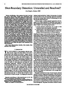
Baseline
Input video
Anchor shot segmentation
shot segmentation
Section-specialized segmentation
feature extraction
section extraction
SVM-based story segmentation
anchor shot extraction
anchor shot segmentation based on “silence”
Post-filter
section-specialized SVM
story boundary addition
Filter candidates w/o silent segments and anchor shots
kddi_ss_c+k1
kddi_ss_all1
kddi_ss_all*pfil*
result output
kddi_ss_base1
Figure 1 Outline of KDDI story segmentation system and official runs.
First, the baseline method frequently overlooks story boundaries that occur in specific sections of the video that have different characteristics from the general content of the video file in question. An example of such sections is the "Top Stories" section of CNN, which, unlike the other portions of the program, contains background music. Furthermore, story changes within the “Top Stories” section occur without anchor shots. Second, the baseline method is incapable of detecting multiple story boundaries that occur within a single shot, such as shots where the anchorperson presents numerous stories successively. In order to solve these problems, and to improve overall story segmentation accuracy, three components were added to the baseline system: (1) Section-specialized segmentation (2) Anchor shot segmentation (3) Post-filtering Figure 1 illustrates the outline of our story segmentation system, and the correlation between each component and officially submitted runs. The following sections provide detailed descriptions of each component.
2.1.2 Section-specialized segmentation As mentioned in the previous section, the recall of the baseline method was significantly poor in specific sections of CNN, such as “Top Stories” and “Headline Sports”. The main cause of this problem is the difference of the characteristics of the specific sections, compared to the general content of the program. While a typical news story features the anchor talking alone in a silent studio environment, stories within the “Top Stories” and “Headline Sports” sections are presented by narration over video reports and background music. Furthermore, the main anchorperson does not appear in both sections. We assumed that the baseline SVM, which is constructed based on the whole development data set, was not able to adapt to the various characteristics of the above sections. In order to increase the recall of story segmentation in these sections, we took the simple approach to develop an SVM specialized to conduct story segmentation within known specific sections. In the training phase, the specific sections, namely, CNN's Top Stories and Headline Sports, are extracted from all files of the development data set. The extracted portions of video are used to construct development data to generate story segmentation SVMs specialized for Top Stories and Headline Sports, respectively. The section-specialized SVMs are then applied to the test data. In order to utilize these SVMs to the test data, it is necessary to automatically extract sections
from each file in the test data set. Automatic section extraction is conducted by applying the "time-series active search" algorithm proposed by Kashino et al[8], which is an efficient and accurate algorithm to detect specific signals from a long signal sequence. In our experiments, we manually extracted the audio signals of the “jingles”, i.e., the introduction and ending music tunes of the Top Stories and Headline Sports sections, from the files in the development data set. The extracted audio signals were then used as reference signals to extract the starting and ending points of the sections in the test data. As a result, we were able to accurately extract approximately 95% of all sections in the test data set. Finally, the section-specialized SVMs are applied to each extracted section, where the story boundaries within the sections are calculated.
2.1.3 Anchor shot segmentation As previously written in Section 2.1.1, the other weak point of the baseline approach is that it is impossible to detect multiple story boundaries within a single shot, since story boundaries can only be set at the start of the extracted shots. Therefore, in order to detect such story boundaries, a method to plot story boundaries within a shot is necessary. Considering the general characteristics of news programs, it is rather obvious that a large majority of shots which contain multiple story boundaries are anchor shots with sufficient length. Therefore, our approach was to first extract long anchor shots from the test data, and segment the extracted anchor shots. Anchor shot extraction was implemented by constructing an anchor shot detection SVM, based on the same features used for the baseline story segmentation method. Table 2 shows the recall, precision, and F-measure of preliminary anchor shot detection experiments, which were conducted on TRECVID 2003 data, using the 2003 development data for training, and the 2003 test data for evaluation. The reference data used for the evaluation of the experiments in Table 2 were constructed manually. Results in Table 2 show that the anchor shot detection SVM is generally achieves high accuracy. The TRECVID 2004 anchor shot detector was generated by using the TRECVID 2003 development and test data for training. Table 2. Recall, precision, and F-measure of anchor shot detection based on TRECVID 2003 data. Recall Precision F-measure ABC 0.859 0.866 0.862 CNN 0.695 0.936 0.798
Next, the extracted anchor shots are segmented based on the detection of “silent sections”, which are assumed to correspond to “pauses” that are inserted by the anchorperson between stories. Silent sections are detected by applying the audio classification algorithm used in the feature extraction process. As previously mentioned in Section 2.1.1, the audio classification algorithm classifies each frame to one of four audio classes: Silence, Noise, Speech, and Music. In this component, we extract consecutive frames classified to the “Silence” class as silent sections. Story boundaries are then inserted at the starting point of each silent section. Furthermore, we also implemented a Hidden Markov Model (HMM) based “non-speech” segment detector, which was also used to segment anchor shots. The non-speech segment detector attempts to classify audio to Male Speech, Female Speech, Silence, Noise, or Music. All audio segments which are not classified as Male or Female speech are extracted as “nonspeech” segments. As in the audio classification approach, story boundaries are inserted at the start of each extracted non-speech segment. The outline of the non-speech segment detector is illustrated in Figure 2.
shot detection methods that were applied in the anchor shot segmentation component are also utilized in the post-filtering component. Condition (1) is based on the observation that story boundaries which occur without significant pause are scarce. There is an obvious tradeoff between recall and precision regarding the candidates that will be omitted based on Condition (2). While a large majority of stories are either initiated or followed by an anchor shot, it is also clear that story boundaries which do not accompany anchor shots also exist. Preliminary experiments were conducted using each of the two conditions independently. However, no improvement could be achieved by the independent implementation of each condition. Therefore, for the official submissions, both conditions were used simultaneously, i.e., only story boundary candidates that fulfill both conditions were omitted in the postfiltering process.
2.2 Experiment results This section presents our TRECVID 2004 story segmentation results, namely results of our official submissions, and comparison of our runs with other non-KDDI runs.
HMMs for speech segments
Male speech Female speech
Silence Noise Music
HMMs for non-speech segments
Figure 2. Outline of HMM-based non-speech segment detector.
2.1.4 Post-filtering In addition to the previously described components, of which the main objective was to increase recall, a postfiltering component was added to improve precision, by omitting suspicious story boundary candidates. The post-filter is a rather naive approach, where story boundary candidates (1) which have no silent segments within its vicinity, and (2) where the shots preceding and following the boundary are both non-anchor shots, are omitted. The silent segment detection and anchor
2.2.1 Results of official KDDI runs Table 3 shows the recall, precision, and F-measure (F1) of all officially submitted “Audio + Video” condition runs from KDDI. The relation between each RunID and their details are presented in the structured abstract. Hereafter, we will refer to each run based on the numbers listed in the first column of Table 3. Table 3. Recall, precision and F-measure of all “Audio + Video” KDDI runs. # 1 2 3 4 5 6 7
RunID 1_kddi_ss_base1_5 1_kddi_ss_c+k1_4 1_kddi_ss_all1_3 1_kddi_ss_all1_pfil_1 1_kddi_ss_all2_pfil_2 1_kddi_ss_all1nsp07_pfil_6 1_kddi_ss_all2nsp07_pfil_7
Recall 0.640 0.707 0.741 0.710 0.756 0.738 0.786
Prec 0.622 0.637 0.630 0.675 0.567 0.642 0.531
F1 0.631 0.670 0.681 0.692 0.648 0.687 0.634
The effects of each component are analyzed by comparing the results of the runs listed in Table 3. Section-specified segmentation (SS-S) By comparison of Runs 1 (Baseline) and 2 (Baseline + SS-S), it is clear that the section-specified segmentation component has achieved approximately 6.7% increase of recall, and 1.5% increase of precision. However, since we could not define any specific sections in ABC,
SS-S was applied only for CNN. Evaluation based only on CNN data showed that the actual increase of recall from the baseline run was 12.3% (60.5% to 72.8%), while the increase of precision was 2.6% (59.6% to 62.5%). These results show that, if it is possible to extract specific sections, the section-specified segmentation method is highly effective to improve recall, without sacrificing precision. Anchor shot segmentation (ASS) By comparing the results of Runs 2 (Baseline + SS-S) and 3 (Baseline + SS-S + ASS), the effect of anchor shot segmentation based on audio classification results can be measured. Since the ASS component naively inserts story boundaries at every detected silence segment, the expected effect is the increase of recall accompanied with the decrease of precision. However, while the overall increase of recall was as expected (+3.4%), the expected decrease of precision was not as significant as predicted (-0.7%). Based on post-analysis of the experiment results, we discovered that silent segments detected by audio classification appear frequently near the end of anchor shots. Many of such detected segments occur within the 5 second buffer of story boundaries, which helped to minimize the negative effects of other mistakenly extracted story boundaries. Post-filtering (PF) Comparison between Run 3 and Runs 4 and 6 show that, as expected, the post-filtering component has achieved improvement of precision. Along with the increase of precision, the recall has decreased, hence, the overall improvement of F-measure was minimal. As mentioned previously, we implemented two methods to detect “silent” sections, which are utilized in the post-filtering process: audio classification and HMM-based non-speech detection. The effects of these two methods can be compared by examining the results of Runs 4 and 6. Generally, the audio classification method achieved higher precision and lower recall compared to HMM-based non-speech detection.
2.2.2 Comparison with non-KDDI runs Next, we compare the performance of our submitted runs with the officially submitted non-KDDI “Audio + Video” runs. Figure 3 illustrates the recall, precision, and F-measure of all official “Audio + Video” story segmentation runs. As clear from the results in Figure 3, our submissions have outperformed all non-KDDI runs. While details regarding the methods used in the nonKDDI runs are not disclosed at the present time, it can be assumed that many of the runs have made use of
news-specific characteristics, such as anchor shot extraction results, as major features for story segmentation. The overall superiority of our results, namely the baseline method, proves that the effective use of low-level audio-video features is sufficient to achieve highly accurate story segmentation.
2.3 Discussions Overall, the results of our story segmentation experiments were satisfying. However, there are some problems which need to be solved in order to implement our method to video data from various domains. One major problem is how to conduct story segmentation on video data when there is insufficient training data. While the recall for ABC was generally high for most of the test data, there were several data where the baseline method could only achieve approximately 10% recall. Post-analysis revealed that the low-recall programs were recorded outside of the usual studio environments, hence, the baseline SVM was incapable to adapt to environment changes which do not appear in the development data set. Another interesting task is to develop a method to automatically extract reference signals for the section detecting algorithm used in the section-specialized segmentation component. As mentioned in Section 2.1.2, the reference signals used to extract specific sections were prepared manually, which is a timeconsuming process. If it becomes possible to input a sufficient amount of video data into an automatic jingle detector, and use the extracted audio/video signals as reference signals for section extraction, the sectionspecialized segmentation method will be applicable to unknown TV programs without deep pre-analysis of the video program in question.
1.0
Recall
0.9
Precision
F-Measure
0.8 0.7 0.6 0.5 0.4 0.3 0.2 0.1
UIowaSS0401_1
rmit4_1
rmit1_1
Imperial-anc-0.43_1
Imperial-anc-0.40_1
Imperial-anc-0.37_1
ibm_mck_av_efc+ec_6
ibm_mck_av_efc+efc_5
ibm_mck_av_fc+fc_8
CLIPS_2
CLIPS_1
kddi_ss_base
kddi_ss_all2nsp07_pfil
kddi_ss_all2_pfil
kddi_ss_c+k1
kddi_ss_all1
kddi_ss_all1nsp07_pfil
kddi_ss_all1_pfil
0.0
Figure 3. Results of all TRECVID 2004 “Audio + Video” official story segmentation runs.
3. SHOT BOUNDARY DETERMINATION This section describes our shot boundary determination methods and experiments. In TV2004, we especially focused on improving recall of gradual shot transitions, as well as precision of abrupt shot boundaries. These modifications are further described in the following subsections.
3.1 Partial MPEG decoding DCT DC coefficients give the lowest frequency component of image and at the same time they represent spatially scaled image since DC component is a block averaged value [9]. Furthermore, in I-pictures these coefficients are directly obtained during VLD (Variable Length Decoding) process without time consuming process such as Inverse DCT. DC components in these pictures can be obtained after some manipulation. In P- and B-pictures, although some of macroblocks may be intra coded, most of the coded blocks are inter coded where only prediction error after motion compensation is coded using DCT. In addition, there may be skip blocks and MC no Coded blocks where no DCT coefficient is coded. DCT DC image is a reduced size image by 1/8 both horizontally and vertically. Therefore DC components of P- and B-pictures are obtained using motion compensation in reduced size image domain.
There are two ways to obtain DCT DC image for P-/Bpictures. One is to apply motion compensation (MC) using reduced size motion vectors in 1/8. The other is to apply weighted motion compensation reflecting contribution of all the blocks used for motion compensation [16][21]. Figure 4 shows a block diagram of the latter scheme. Subjectively, it is found that the latter has less visible noise due to motion compensation mismatch. Therefore we use the latter method to obtain DCT DC images for P- and Bpictures. MPEG Coded Stream
VLD
DCT DC Reconst.
8×8 Block Average
Weighted MC
DC image for I, B, P
Frame Memory
Figure 4. DC image with weighted MC
3.2 Shot boundary determination methods 3.2.1 Abrupt shot boundary determination By incorporating the MC operation mentioned above, P- and B-pictures are roughly reconstructed so that temporal resolution can be greatly improved. Previously a good deal of research work has been
reported on shot boundary determination. The major technique includes pixel differences, histogram comparison, edge differences statistical differences, compressed data amount differences, and motion vectors. Although either one of the above techniques achieves relatively high accuracy, each has its own disadvantage [2]. We proposed shot boundary determination from Ipicture sequence of MPEG coded video in 1994 [9]. We use both pixel differences and histograms methods to overcome problems when either one of them is used. Here, we extend this approach to detect shot boundaries in one frame unit. Pre-processing To exclude undesired false detection mainly due to camera motion and object movement, only frames with high inter-frame difference are picked up for the succeeding shot boundary determination. The interframe difference is obtained by: M
N
Dn = ∑∑ Yn (i, j ) − Yn −1 (i, j )
(1)
i =0 j =0
, where M and N are total number of 8×8 blocks in a frame for vertical and horizontal direction, respectively. For example, in MPEG-1 in SIF size (352×240), M=30 and N=44. Yn(i,j) is the luminance block average at block (i,j) in the n th frame. Since DCT DC component of each 8×8 block is obtained from section 2, Yn(i,j) for each frame is directly given from this value. Then the following equation is used as pre-processing: Dn > Th_pre
(2)
Only those frames which satisfy the above conditions are further investigated in abrupt shot boundary detection in the following.
Shot boundary determination using luminance and chrominance change Both luminance and chrominance characteristics dramatically change at shot boundaries. Thus ordinary shot boundaries are detected when both the luminance and chrominance information greatly change. We use temporal peak detection of both inter-frame luminance difference and chrominance histogram correlation [9]. A frame is declared as a shot boundary when: αDn > Dn - 1, Dn + 1 and ρn > ρn - 1, ρn + 1
(3)
Here, α is a weighting factor for the detection. ρn is chrominance histogram correlation obtained by:
ρn =
∑H
n ,k ,l
H n−1,k ,l
k ,l
1/ 2
⎛ ⎞ ⎜⎜ ∑ H n ,k ,l 2 ∑ H n−1,k ,l 2 ⎟⎟ k ,l ⎝ k ,l ⎠
(4)
, where Hn,k,l is a chrominance histogram matrix. The histogram is obtained classifying DC chrominance Cb and Cr data in a frame into hc classes for each chrominance component. Then two dimensional hc×hc histogram matrix in the n-th frame Hn,k,l (k, l = 0, 1, 2... hc-1) is obtained. When shot boundary exists on scenes with large motion, it is very difficult to find temporal peak using frame difference since frame difference may be very large all the way due to motion so that Eq. (3) may not detect such shot boundaries. Therefore, only chrominance correlation is used to detect such shot boundary for those frames which do not satisfy Eq. (3).
ρn > Th_ac
(5)
, where Th_ac is a threshold value for determination of temporal peak in ρn. Furthermore, when consecutive two shots are different only in camera angle, color histogram will be similar and thus it is difficult to detect shot boundary by the above conditions such as Eq. (3) and (5). However, since pixel difference usually has a very large peak at these shot boundaries, peak detection of luminance difference are applied. When either of the following equation is satisfied for those frames which are not declared as scene change in the above process, the frame is declared as shot boundary. βDn > Dn - 1, Dn + 1 Dn – Th_ad > Dn - 1, Dn + 1
(6) (7)
, where β and Th_ad are a weighting factor and a threshold value for detecting a temporal peak in Dn, respectively. Basically, Eq. (6) will detect shot boundaries in similar scenes. However, Eq. (7) is also used for such cases when motion is involved since all of the inter-frame differences are kept relatively high and the ratio of Dn to Dn-1 or Dn+1 may not be significantly high enough to find the shot boundary using Eq. (6).
Shot boundary determination between fields in a progressive sequence TRECVID test data are encoded by MPEG-1, i.e. encoded as progressive sequences, while the source materials (CNN/ABC news videos) are captured as interlaced sequences. Therefore some abrupt shot boundaries between the different fields in a progressive
image appears in the test data. That is, a top field belongs to the previous shot while a bottom field belongs to the next shot. In order to detect such abrupt shot boundaries correctly, we determine the n-th frame as CUT between fields on following conditions: -
If adjacent frames are determined to have very large Dn and low edge histogram correlation εn (see 3.2.2.) If ρ(n, n-2), the chrominance histogram correlation between the n-th frame and (n-2)-th frame is low and Dn is large.
Each threshold value is obtained from training data (TRECVID 2003 test data).
Post-processing for deleting non-CUT For the purpose of improving precision for CUT, we optionally applied post-processing for deleting nonCUT candidates, which is based on non-CUT learning method using development data. More specifically, non-CUT shot boundaries were manually extracted from the initial CUT candidates results, and behaviors of each parameter on non-CUT were learned. Based on learning, for each sequence, we applied the top 50 nonCUT candidates to the intermediate results. Then after deleting non-CUT results, the final CUT results were formed.
3.2.2 Dissolve shot boundary determination Basic detection algorithm of dissolve and fade In gradual transition such as dissolve and fade in/out, two different shots are usually synthesized in the course of transition. For example, in dissolve transition, gradual change from one shot to another occurs with simultaneous decrease and increase of intensities of preceding and following shots. Since both shots are synthesized during transition, activity of the each frame shows U-shape curve surrounded by flat shoulders when dissolve occurs [14]. In the case of fade in/out, activity curve shows monotonous increase/decrease. The frame activity for n-th frame FAn is described as: M
N
FAn = ∑∑ Yn (i, j ) 2 − Yn (i, j ) i =0 j =0
2
(8)
In [20], the positive peak before dissolve and the negative peak during dissolve are used to detect Ushape variance curve. It assumes that only single pair of positive and negative peaks with a large peak to peak difference exists during dissolve period. However, in the actual video sequences, it rarely shows these shapes due to motion and local fluctuations. However it
is difficult to find real positive and negative peaks of dissolve region even if the variance shows U-shape curve [2]. Furthermore, peak to peak difference may not always be large due to picture flatness or motion. In order to detect these shapes avoiding false detection, we have applied filtering process as noise reduction for the DCT DC activity data. Since dissolve and fade processes take long duration, temporal filtering with long tap is suitable to absorb spontaneous fluctuations and examine long duration variation. As a temporal filtering, we use a moving average of activities MAn for a period of frames VF which includes current and previous (VF -1) frames: MAn =
1 VF
n−VF +1
∑ FA t =n
t
(9)
After temporal filtering, temporal peak or monotonous increase/decrease can be detected. However, since duration of dissolve and fade depends on how the shots are edited, such a technique as simple peak detection may result in false detection. Furthermore, very flat Ushape curve will be expected when a dissolve transition occurs in between relatively flat shots. Therefore it is necessary to contrast these curves with others. We use first order derivative of the filtered activity DAn in order to detect these curves. It is obtained as: DAn = MAn − MAn−1
(10)
In TRECVID data, the derivative curve tends to be negative in our preliminary experiment. Therefore dissolve period are found when the derivative curve continuously takes negative values during a certain period. Fade in/out period can also be found when only positive/negative period is detected. In order to exclude undesired detection in such scenes as motion, we use chrominance correlation between n-th and (n-dd)-th frames to confirm that the region is a shot boundary candidate. Therefore dissolve sequence candidates are detected using the following equations. DAn < -Th_dis1 and ρn, n - dd < Th_dis2
(11)
Between n-th and (n-dd)-th frame, if the number of frames satisfying Eq. (11) is larger than Th_dis3, a dissolve transition is determined in this period. In order to avoid detecting motion scenes, the following equation should be considered: k < Th_dis4
(12)
, where k is number of non-intra blocks. Dissolve detection is carried out for those frames which are determined as non abrupt scene change in the previous section.
Although the above equations can detect most of the dissolve shot transitions, there are two problems in terms of detection accuracy. One is that it is difficult to detect those dissolve transitions in similar color shots or in shots with large flat areas, since conditions in Eq. (11) assumes that two shots have different color distributions with non-flat regions. The other is that it may also detect panning or motion scenes as dissolving since these scenes may have similar activity curve in such cases when scenes with large flat object appear during panning. In the following, countermeasures for these errors in the detection are described.
that period. An instance of Color Layout Descriptor is a set of DCT coefficients of Y, Cb, and Cr component of downscaled (8×8) frame. This strategy is used together with other dissolve transition decision strategies. 3.2.3 Wipe shot boundary determination Since our wipe shot boundary determination algorithm has not been changed since TV2003, the detailed descriptions are left out from this paper. Refer to [22] for details of our wipe shot boundary determination algorithm. n
Dissolve determination based on edge features This algorithm has been newly introduced in TV2004, in order to improve recall of dissolves and fades. Based on the observations that edge feature becomes weak during fades or dissolves, we used edge features for determining fade/dissolve transitions. More specifically, two edge features derived from Edge Histogram Descriptor specified in MPEG-7 Visual [6] is extracted from DC images described above. Thus computational complexity for obtaining edge feature is very low. At first DC image is divided into 4×4 sub-images, and for each sub-images 5 types of directional filters are applied, which results in 5 bins of directional histogram. For determining fades and dissolves, the edge power EP for each frame and the edge histogram correlations εn between adjacent frames are used together with above DAn and NPEn. That is, since the edge power EP shows U-shape curve and the edge histogram correlations εn is larger than Th_eh during dissolve period, these observations can determine fade or dissolve transitions at high recall. Dissolve determination between shots with similar color characteristic In TV2004, we added new determination strategy for determining dissolve transitions between adjacent shots with very similar color characteristic. This is because in the TV2003, these types of dissolve transitions were not successfully determined. Basically the luminance difference and chrominance histogram correlation are only the factors for decision, spatial characteristic of color information has been newly incorporated; Color Layout Descriptor defined in MPEG-7 Visual[6]. That is, at gradual transition where adjacent shots have similar color characteristic, although an obvious change is not observed in terms of chrominance histogram, the color layout is more likely to change. Thus we observed the difference of Color Layout values ∆CL for each frame, and if ∆CL > Th_cl is satisfied during a certain period, we determine that dissolve transition is contained in
n-1 L
L H (a) Flashlight/subliminal at n-th frame
H
L
(b) Flashlight/subliminal at n-1-th frame
Figure 4. Single flashlight/subliminal effect models
2.2.4 Flashlight and subliminal effect detection A flashlight scene is spontaneous frame change due to flashlight in a shot. For example, in TV news sequence, a flashlight scene appears while an important person gives a speech in a press conference. Also a subliminal effect (simply subliminal, hereafter) may be inserted into TV programs or films with a certain intention. Since a flashlight frame and a subliminal frame are quite different from preceding and following frames, frames with flashlight/subliminal and after flashlight/ subliminal are often falsely detected as scene change. Luminance and chrominance distributions in flashlight/ subliminal frame are completely different from those in the previous frames. However, unlike shot boundary, these distributions in flashlight return to the previous states after one or a few frames. Therefore by investigating frames before and after flashlight scene, flashlight scene can be excluded from scene change points. Single flashlight model is depicted in Figure 4. For example, when n-th frame is flashlight scene, correlation between n-th and n-1-th is low whereas correlation between n+1 and n-1 is high as shown Figure 4(a). In the same way, especially consecutive flashlight scenes can be easily modeled by extending single flashlight model. We use chrominance histogram correlation as correlation measure in order to distinguish flashlight from other shot boundary. Therefore flashlight/subliminal effect at n-th frame is detected when:
ρ (n , n - 1) < Th _fl , ρ (n +1, n -1) > Th _fh
(24)
In TRECVID 2004, furthermore, we extended this idea to consecutive, multiple flashlights (N flashlights) detection. Based on the above equation, while the n-th frame satisfies:
ρn > Th_mfl and ρn-1 > Th_mfl
(25)
, a sequence of corresponding frames are regarded as being a multiple flashlights candidate, and the chrominance histogram correlation between the frames just before/after the above sequence is higher than a predefined threshold, the multiple flashlights are declared and omitted from CUT results.
3.3 Evaluation results We applied the above mentioned shot boundary determination to TRECVID 2004 test data (totally 12 sequences). All the parameters used in the above equations are determined through TRECVID 2003 test data. Tables 4 through 6 show the results of shot boundary determination; recall, precision, and Fmeasure for ALL, CUT, and GRAD results for submitted 6 runs. The relation between each RunID and their details are presented in the structured abstract. As shown in Table 5, most of abrupt shot boundaries are successfully detected. However, in spite of incorporating flashlight exclusion algorithm, most of the false detections for abrupt shot boundaries are flashlights. In addition, sudden changes of brightness such as shining are falsely determined as abrupt shot boundaries. As for un-detection, the abrupt shot boundaries between fields are not detected since the test data is encoded in frame structures. Also the shot boundaries where the frame is only partly changed are not detected. As for gradual transitions, using edge features greatly improved recall. In our internal evaluation, the recall gain is about 11% on average, and more than 20% at maximum. However, over 30% of gradual transitions are still undetected. These misdetections are mainly caused by the following: i) Shot boundaries between black-and-white shots. ii) Shot boundaries between relatively dark shots. iii) Shot boundaries which occur on not entire image, e.g. when the upper and bottom portions of an image is unchanged such as closed captions and market information, while a shot changes occurs in the middle of the image.
Actually these reasons apply not only for gradual transitions, but also abrupt transitions. In addition, in spite of incorporating multiple flashlights detection algorithm, many of multiple flashlights were not determined. This is because brightness of flashlights during multiple flashlights generally changes. As for computational cost, our method achieves very fast operation, about 923.34 frames/second for processing on the normal Windows PC with Pentium 4 1.8GHz CPU and 512MB RAM, since all the processes are performed on compressed data domain.
Table 4. Recall, precision and F-measure of ALL # 1 2 3 4 5
RunID kddi_labs_sb_run_01 kddi_labs_sb_run_06 kddi_labs_sb_run_07 kddi_labs_sb_run_09 kddi_labs_sb_run_10
Recall 0.833 0.827 0.834 0.734 0.645
Precision 0.808 0.790 0.801 0.551 0.526
F1 0.820 0.808 0.817 0.629 0.579
Table 5. Recall, precision and F-measure of CUT # 1 2 3 4 5
RunID kddi_labs_sb_run_01 kddi_labs_sb_run_06 kddi_labs_sb_run_07 kddi_labs_sb_run_09 kddi_labs_sb_run_10
Recall 0.916 0.893 0.917 0.830 0.683
Precision 0.861 0.877 0.851 0.862 0.915
F1 0.888 0.885 0.883 0.846 0.782
Table 6. Recall, precision and F-measure of GRAD # 1 2 3 4 5
RunID kddi_labs_sb_run_01 kddi_labs_sb_run_06 kddi_labs_sb_run_07 kddi_labs_sb_run_09 kddi_labs_sb_run_10
Recall 0.658 0.687 0.660 0.531 0.564
Precision 0.683 0.622 0.683 0.252 0.252
F1 0.670 0.653 0.671 0.341 0.348
3.4 Conclusion In this Section, firstly the preprocessing method for shot boundary determination is described. By using motion vectors and DCT DC information, DC image in 1/64 of original coded sized has been obtained directly from MPEG bitstream for P- and B-pictures as well as I-pictures. Shot boundary determination algorithm not only for abrupt scene change but also for gradual transitions is proposed. In our methods, statistics such as histograms as well as motion vectors extracted from coded bitstream are used to adaptively detect various types of shot boundaries. In addition, exclusion algorithms for panning and flashlight/subliminal scenes have also been proposed. In the experiment around 95% of abrupt shot boundaries are successfully detected for the TRECVID test data. As for gradual transitions, about half of shot boundaries are detected. Since the shot detection process is very fast and only
less than 5% of normal playback time is required, the proposed method well realizes efficient shot boundary determination, which can be used for higher level processing such as content-based video analysis.
4. REFERENCES [1] J.L. Gauvain, L. Lamel, and G. Adda. The LIMSI Broadcast News Transcription System., Speech Communication, 37(1-2):89-108, 2002. ftp://tlp.limsi.fr/public/spcH4_limsi.ps.Z [2] Y. Nakajima, K. Ujihara, and A. Yoneyama, "Universal scene change detection on MPEG-coded data domain," in Proceeding SPIE Visual Communications and Image Processing, vol. 3024, pp. 992-1003, 1997. [3] V. Vapnik: “Statistical learning theory”, A WileyInterscience Publication, 1998. [4] C.-Y. Lin, B. Tseng, and J.R. Smith, “Video Collaborative Annotation Forum: Establishing Ground-Truth Labels on Large Multimedia Datasets,” Proc of TRECVID 2003, http://www-nlpir.nist.gov/projects/tvpubs/papers/ ibm.final2.paper.pdf, 2003. [5] Y. Nakajima, Y. Lu, M. Sugano, A. Yoneyama, H. Yanagihara, A. Kurematsu: “A fast audio classification from MPEG coded data”, Proc. ICASSP ’99, Vol.6, pp 3005-3008, 1999. [6] ISO/IEC 15938-3, “Information Technology --Multimedia content description interface – Part 3: Visual”, 2002. [7] M. Sugano, Y. Nakajima, H. Yanagihara: “MPEG content summarization based on compressed domain feature analysis”, Proc. SPIE Int’l Symposium ITCom2003, Vol 5242, pp 280-288, 2003. [8] K. Kashino, T. Kurozumi, and H. Murase: “A quick search method for audio and video signals based on histogram pruning,” IEEE Trans Multimedia, Vol 5, Issue 3, pp 349-355, 2003. [9] Y. Nakajima, "A Video Browsing Using fast scene change detection for an efficient networked video database access," IEICE Transactions on Information & Systems, vol.E-77-D, No.12, pp.1355-1364, Dec.1994. [10] Y. Tonomura, A. Akutsu, Y. Taniguchi, and G. Suzuki, "Structured video computing," IEEE Multimedia, pp.34-43, Fall 1994. [11] K. Otsuji and Y. Tonomura, "Projection detecting filter for video cut detection", Proceedings of First ACM International Conference on Multimedia, pp.251-257, Aug.1993 [12] H. J. Zhang, A. Kankanhalli, and S. W. Smoliar, "Automatic parsing of news video," Proc.IEEE Int’l Conf. Multimedia Computing and Systems, May. 1994. [13] S. W. Smoliar and H. J. Zhang, "Content-based video indexing and retrieval," IEEE Multimedia, pp.62-72, 1994. [14] A. Nagasaka and Y. Tanaka, "Automatic video indexing and full-motion search for object appearances", Visual database systems, Vol.II, E.Knuth and L.M.Wegner, eds, Elsevier, Amsterdam, pp.113-127, 1992. [15] F. Arman, R. Depommier, A. Hsu, and M. Y. Chiu, "Image processing on compressed data for large video
databases", Proceedings of First ACM International Conference on Multimedia, pp.267-272, Aug.1993. [16] B. L. Yeo and B. Liu, "Rapid scene analysis on compressed video", IEEE Transactions on Circuits and Systems for Video Technology, Dec.1995. [17] B. Shahrarary, "Scene change detection and contentbased sampling of video sequences", Digital Video Compression: Algorithms and Technologies, SPIE, Vol.2419, pp.2-13, 1995. [18] A. Hampapur, R. Jain and T. Weymouth, "Digital Video Segmentation", Proc. ACM Multimedia 94, pp.357-364, 1994. [19] K. Shen and E. J. Delp, "A Fast Algorithm for Video Parsing Using MPEG Compressed Sequences", Proceeding of IEEE ICIP ‘95, pp.252-255, 1995. [20] J. Meng, Y. Juan and S-F Chang, "Scene Change Detection in a MPEG Compressed Video Sequence", Digital Video Compression: Algorithms and Technologies, SPIE, Vol.2419, pp.14-25, 1995. [21] Y. Nakajima, K. Ujihara, and T. Kanoh, "Video structure analysis and its application to creation of video summary", IEICE 2nd Joint Workshop on Multimedia Communications, pp.3-2, Oct.1995. [22] M. Sugano, K. Hoashi, K. Matsumoto, F. Sugaya, and Y. Nakajima: Shot boundary determination on MPEG compressed domain and story segmentation experiments for TRECVID 2003, Proc of TRECVID 2003, http://wwwnlpir.nist.gov/projects/tvpubs/papers/kddi.final2.paper.pdf, 2003.