Description: Sigmoid dose-response logistic function, predicting the viral transduction dynamics (f(x)td) and viral titre (f(x)vt),. % was implemented in the MATLAB ...
% % % % % % % % %
Description: Sigmoid dose-response logistic function, predicting the viral transduction dynamics (f(x)td) and viral titre (f(x)vt), was implemented in the MATLAB script M-files using the following equations: f(x)_td= 0.01a/(0.01+e^((-bx) ) ) and f(x)_vt= a/(0.01+e^x ), where x is any independent variable described by linspace function; a is a transduction rate (percentage of eGFP cells); e is an exponential constant (e = 2.718); and b integer is a Hill Slope. The linspace function (x = linspace (0, 48)) was used to generate linearly spaced vectors for 48-hour interval curve. The b integer (b = 0.21) was adjusted to the f(x)td logistic function for pWPXL (y1=1.0./(0.01+exp(-x.*0.21)) as a reference curve reaching the upper plateau level with maximal effect after 48 hrs. To determine the viral titre dynamics, seven dilutions were inspected in the range from the highest (0.1) to the lowest (10-7) concentrations of the virus (x = linspace (0, 6)).
subplot (3,3,1) x=linspace(0,48); y1=1.0./(0.01+exp(-x.*0.21)); y2=0.9367./(0.01+exp(-x.*0.21)); y3=0.0./(0.01+exp(-x.*0.21)); y4=0.0./(0.01+exp(-x.*0.21)); y5=0.5101./(0.01+exp(-x.*0.21)); y6=0.8143./(0.01+exp(-x.*0.21)); y7=0.7334./(0.01+exp(-x.*0.21)); y8=0.8663./(0.01+exp(-x.*0.21)); plot(x,y1,'black--',x,y2,'black-.',x,y3,'magenta',x,y4,'cyan',x,y5,'black',x,y6,'blue',x,y7,'green',x,y8,'red','LineWidth',2); % legend('pWPXL','pMD9','pMD9-(w/oEnv)','pcDNA','pMD9-cPPT(HIV)-CTS','pMD9-cPPT(PFV)-CTS','pMD9-cPPT(HIV)','pMD9-CTS','Location','NorthWest'); ylabel('eGFP Cells (%)','FontSize',10); xlabel('Time (hrs)','FontSize',10); set(gca,'XTick',0:8:48); set(gca,'YTick',0:20:100); xlim([0 48]) grid on hold on subplot (3,3,2) x=linspace(0,48); y1=1.0./(0.01+exp(-x.*0.21)); y2=0.8724./(0.01+exp(-x.*0.21)); y3=0.0./(0.01+exp(-x.*0.21)); y4=0.0./(0.01+exp(-x.*0.21)); y5=0.4533./(0.01+exp(-x.*0.21)); y6=0.7741./(0.01+exp(-x.*0.21)); y7=0.7183./(0.01+exp(-x.*0.21)); y8=0.6473./(0.01+exp(-x.*0.21)); plot(x,y1,'black--',x,y2,'black-.',x,y3,'magenta',x,y4,'cyan',x,y5,'black',x,y6,'blue',x,y7,'green',x,y8,'red','LineWidth',2); % legend('pWPXL','pMD9','pMD9-(w/oEnv)','pcDNA','pMD9-cPPT(HIV)-CTS','pMD9-cPPT(PFV)-CTS','pMD9-cPPT(HIV)','pMD9-CTS','Location','NorthWest'); ylabel('eGFP Cells (%)','FontSize',10); xlabel('Time (hrs)','FontSize',10); set(gca,'XTick',0:8:48); set(gca,'YTick',0:20:100); xlim([0 48]) grid on hold on subplot (3,3,3) x=linspace(0,48); y1=1.0./(0.01+exp(-x.*0.21)); y2=0.1679./(0.01+exp(-x.*0.21)); y3=0.0./(0.01+exp(-x.*0.21)); y4=0.0./(0.01+exp(-x.*0.21)); y5=0.0465./(0.01+exp(-x.*0.21)); y6=0.1313./(0.01+exp(-x.*0.21)); y7=0.1468./(0.01+exp(-x.*0.21)); y8=0.2055./(0.01+exp(-x.*0.21)); plot(x,y1,'black--',x,y2,'black-.',x,y3,'magenta',x,y4,'cyan',x,y5,'black',x,y6,'blue',x,y7,'green',x,y8,'red','LineWidth',2); % legend('pWPXL','pMD9','pMD9-(w/oEnv)','pcDNA','pMD9-cPPT(HIV)-CTS','pMD9-cPPT(PFV)-CTS','pMD9-cPPT(HIV)','pMD9-CTS','Location','NorthWest'); ylabel('eGFP Cells (%)','FontSize',10); xlabel('Time (hrs)','FontSize',10); % text(24.5,25,['Aphidicolin']) set(gca,'XTick',0:8:48); set(gca,'YTick',0:20:100); xlim([0 48]) grid on hold on subplot (3,3,4) x=linspace(0,6); y1=100.0./(0.01+exp(x)); y2=93.67./(0.01+exp(x)); y3=0.0./(0.01+exp(x)); y4=0.0./(0.01+exp(x)); y5=51.01./(0.01+exp(x)); y6=81.43./(0.01+exp(x)); y7=73.34./(0.01+exp(x)); y8=86.63./(0.01+exp(x)); plot(x,y1,'black--',x,y2,'black-.',x,y3,'magenta',x,y4,'cyan',x,y5,'black',x,y6,'blue',x,y7,'green',x,y8,'red','LineWidth',2); % legend('pWPXL','pMD9','pMD9-(w/oEnv)','pcDNA','pMD9-cPPT(HIV)-CTS','pMD9-cPPT(PFV)-CTS','pMD9-cPPT(HIV)','pMD9-CTS','Location','NorthEast'); ticks=['10^-1';'10^-2';'10^-3';'10^-4';'10^-5';'10^-6';'10^-7']; ylabel('eGFP Cells (%)','FontSize',10); xlabel('Dilution','FontSize',10);
converted by Web2PDFConvert.com
set(gca,'YTick',0:20:100); set(gca,'XTickLabel',ticks) xlim([0 6]) grid on hold on subplot (3,3,5) x=linspace(0,6); y1=100.0./(0.01+exp(x)); y2=87.24./(0.01+exp(x)); y3=0.0./(0.01+exp(x)); y4=0.0./(0.01+exp(x)); y5=45.33./(0.01+exp(x)); y6=77.41./(0.01+exp(x)); y7=71.83./(0.01+exp(x)); y8=64.73./(0.01+exp(x)); plot(x,y1,'black--',x,y2,'black-.',x,y3,'magenta',x,y4,'cyan',x,y5,'black',x,y6,'blue',x,y7,'green',x,y8,'red','LineWidth',2); % legend('pWPXL','pMD9','pMD9-(w/oEnv)','pcDNA','pMD9-cPPT(HIV)-CTS','pMD9-cPPT(PFV)-CTS','pMD9-cPPT(HIV)','pMD9-CTS','Location','NorthEast'); ticks=['10^-1';'10^-2';'10^-3';'10^-4';'10^-5';'10^-6';'10^-7']; ylabel('eGFP Cells (%)','FontSize',10); xlabel('Dilution','FontSize',10); set(gca,'YTick',0:20:100); set(gca,'XTickLabel',ticks); xlim([0 6]) grid on hold on subplot (3,3,6) x=linspace(0,6); y1=100.0./(0.01+exp(x)); y2=16.79./(0.01+exp(x)); y3=0.0./(0.01+exp(x)); y4=0.0./(0.01+exp(x)); y5=4.65./(0.01+exp(x)); y6=13.13./(0.01+exp(x)); y7=14.68./(0.01+exp(x)); y8=20.55./(0.01+exp(x)); plot(x,y1,'black--',x,y2,'black-.',x,y3,'magenta',x,y4,'cyan',x,y5,'black',x,y6,'blue',x,y7,'green',x,y8,'red','LineWidth',2); % legend('pWPXL','pMD9','pMD9-(w/oEnv)','pcDNA','pMD9-cPPT(HIV)-CTS','pMD9-cPPT(PFV)-CTS','pMD9-cPPT(HIV)','pMD9-CTS','Location','NorthEast'); ticks=['10^-1';'10^-2';'10^-3';'10^-4';'10^-5';'10^-6';'10^-7']; ylabel('eGFP Cells (%)','FontSize',10); xlabel('Dilution','FontSize',10); set(gca,'YTick',0:20:100); set(gca,'XTickLabel',ticks) xlim([0 6]) grid on
Published with MATLAB® 7.14
converted by Web2PDFConvert.com