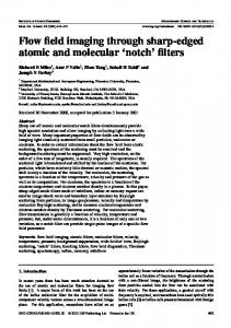
3.4: Contour plots of a slide through the 3D symmetrized ACF; left: Yosemite ... true optical flow: Yosemite (without clouds) diverging tree and translating tree.
Signal and Noise adapted Filters for Differential Motion Estimation Kai Krajsek and Rudolf Mester J. W. Goethe University, Frankfurt, Germany {krajsek, mester}@iap.uni-frankfurt.de http://www.cvg.physik.uni-frankfurt.de/
Abstract. Differential motion estimation in image sequences is based on measuring the orientation of local structures in spatio-temporal signal volumes. Filters estimating the local gradient are applied to the image sequence for this purpose. Whereas previous approaches to filter optimization concentrate on the reduction of the systematical error of filters and motion models, the method presented in this paper is based on the statistical characteristics of the data. We present a method for adapting linear shift invariant filters to image sequences or whole classes of image sequences. Therefore, it is possible to simultaneously optimize derivative filters according to the systematical errors as well as to the statistical ones.
1
Introduction
Many methods have been developed to estimate the motion in image sequences. A class of methods delivering reliable estimates [1] are the differential based motion estimators containing a wide range of different algorithms [1,2,3]. All of them are based on approximation of derivatives on a discrete grid and it turns out that this approximation is an essential key point in order to achieve precise estimates [1,4]. Many different methods have been developed in the last decade trying to reduce the systematical approximation error [5,6,7,8,9,10]. The fact that all real world images are corrupted by noise has been neglected by these methods. In extension to these approaches we propose a prefilter adapted to the statistical characteristics of the signal and the noise contained in it. 1.1
Differential approaches to motion analysis
The general principle behind all differential approaches to motion estimation is that the conservation of some local image characteristic throughout its temporal evolution is reflected in terms of differential-geometric descriptors. In its simplest form, the assumed conservation of brightness along the motion trajectory through space-time leads to the well-known brightness constancy constraint equation (BCCE), where ∂s(x)/∂r denotes the directional derivative in direction r,|r| = 1 and g(x) is the gradient of the gray value signal s(x): ∂s(x) =0 ∂r
⇔
g T (x) · r = 0.
(1)
Since g T (x) · r is identical to the directional derivative of s in direction r, the BCCE states that this derivative vanishes in the direction of motion. Since it is fundamentally impossible to solve for r by a single linear equation additional constraints have to be considered. One way to cope with the so called aperture problem is to perform a weighted average of multiple BCCE’s in a local neighborhood V . Using a spatiotemporal weighting function w(x) and the Euclidean metric this leads to the optimization problem Z 2 w(x) g T (x) · r dx −→ min V Z ⇒ r T Cg r −→ min with Cg := w(x)g(x)g T (x) dx. V
The solution vector rˆ is the eigenvector corresponding to the minimum eigenvalue of the structure tensor Cg (cf. [11,12]). In order to calculate the structure tensor, the partial derivatives of the signal has to be computed at discrete grid points. The implementation of the discrete derivative operators itself is a formidable problem, even though some early authors [2] apparently overlooked the crucial importance of this point. 1.2
Discrete derivative operators
Since derivatives are only defined for continuous signals, an interpolation of the discrete signal s(xn ), n ∈ {1, 2, ..., N }, xn ∈ IR3 to the assumed underlying continuous signal s(x) has to be performed [5] where c(x) denotes the continuous interpolation kernel � � X ∂ X ∂ ∂s(x) = s(xj )c(x − xj ) = s(xj ) c(x − xj ) .(2) ∂r xn ∂r ∂r xn j j | {z } xn dr (xn )
The right hand side of eq. (2) is the convolution of the discrete signal s(xn ) with the sampled derivative of the interpolation kernel dr (xn ), the impulse response n) of the derivative filter ∂s(x = s(xn ) ∗ dr (xn ). Since an ideal discrete derivative ∂r filter dr (xn ) has an infinite number of coefficients [13], an approximation dˆr (xn ) has to be found. In an attempt to simultaneously perform the interpolation and some additional noise reduction by smoothing, often Gaussian functions are used as interpolation kernels c(x) [12]. In the next section we show how to get rid of such ad hoc approaches. Instead of choosing a Gaussian function in order to reduce assumed(!) noise in high frequency regions we derive a signal and noise adapted filter whose shape is determined by the actual signal and noise characteristic.
2
The Signal and Noise adapted Filter approach
The signal and noise adapted (SNA)-filter approach is motivated by the fact that we can exchange the directional derivative filter dr (xn ) in the BCCE by
any other steerable filter hr (xn ) which only nullifies the signal when applied in the direction of motion. The shape of the frequency spectrum of any rank 2 signal is a plane Kr going through the origin of the Fourier space and its normal vector n points to the direction of motion r [12]. Thus, the transfer function 1 Hr (f ) has to be zero in that plane, but the shape of Hr (f ) outside of plane Kr can be chosen freely as long as it is not zero at all. If the impulse response hr (xn ) shall be real-valued, the corresponding transfer function Hr (f ) has to be real and symmetric or imaginary and antisymmetric or a linear combination thereof. The additional degrees of freedom to design the shape outside Kr make it possible to consider the spectral characteristics of the signal and the noise encoded in the second order statistical moments in the filter design. In the following section the derivative of an optimal filter is shown which is a special case of the more general framework presented in [?].
2.1
General model of the observed signal
The general idea of the SNA-filter is to combine Wiener’s theory of optimal filtering with a desired ideal impulse response. Ideal, in this case, means that the filter is optimized with respect to the ideal noise free signal s(x). But signals are always corrupted by noise. Our goal is now to adapt the ideal filter hr (x) to more realistic situations where signal are corrupted by noise. We model the observed image signal z at position i, j, k in a spatio-temporal block of dimension N × N × N by the sum of the ideal (noise free) signal s and a noise term v: z(i, j, k) = s(i, j, k) + v(i, j, k). For the subsequent steps, it is convenient to arrange the s, v, and z of the block in vectors s ∈ IRM , v ∈ IRM and z ∈ IRM . Filtering this ‘vectorized’ pixel set z can thus be written as scalar product gˆ = xT z using a filter coefficient vector x ∈ IRM . The block diagram in fig. 2.1 provides a graphical representation of our model, and the corresponding equation for the actual filter output gˆ reads: gˆ = xT z = xT ( s + v) = x T s + x T v .
(3)
Our task is to choose x T in such a way that the filtered output gˆ approximates, on an average, the desired output g = hT s for the error-free case as closely as possible. The next step is to define the statistical properties of the signal and N the noise processes, respectively. Let the� noise � vector v ∈ IR be a zero-mean T random vector with covariance matrix E vv = Cv (which is in this case equal to its correlation matrix Rv ). Furthermore, we assume that the process that generated the signal s ∈ IRN can be described by the expectation E [s] = ms � � of the signal vector, and an autocorrelation matrix E� ssT� = Rs . Our last assumption is that noise and signal are uncorrelated E sv T = 0. 1
Note that the Fourier transforms of functions are denoted by capital letters.
Fig. 2.1: Block diagram of the filter design scenario (unobservable entities in the dashed frame)
2.2
Designing the optimized filter
Knowing these first and second order statistical moments for both the noise as well as the signal allows the derivation of the optimum filter x. Next, we define the approximation error e := gˆ − g between the ideal output g and the actual output gˆ. The expected squared error Q as a function of the vector x can be computed from the second order statistical moments: � � � � � � Q(x) = E e2 = E gˆ2 − 2E [gˆ g] + E g2 = h T Rs h − 2xT Rs + x T (RsT + Rv )x We see that a minimum mean squared error (MMSE) estimator can now be designed. We set the derivative ∂Q(x)/∂x to 0 and after solving for x we obtain x = (RsT + Rv )−1 Rs h = Mh . | {z }
(4)
M
Thus, the desired SNA-filter is obtained by a matrix vector multiplication. The ideal filter designed for the ideal noise free case is multiplied with a matrix composed out of the correlation matrices of signal and noise.
3
Designed filter sets
With the framework presented in section 2 we are able to find for each linear shift invariant filter h a corresponding noise resistance filter operator which takes into account the 2nd order statistics. In order to obtain optimal results also for low signal to noise ratios, h should be already optimized for the noise free case.
We use filters optimized by the methods of Scharr [7] and Simoncelli [5]. The methods of Elad et al.[9] and Robinson and Milanfar [10] use prior information about the velocity range (before the motion estimation!) which is not guaranteed to be available in all applications. If this information is available it should be used to adapt the filter to it. However, our approach is already adapted to the motion range reflected in the autocorrelation function of the image sequence which can easily be estimated. For comparison reasons we also optimize the 5 × 5 × 5 Sobel operator, which is clearly a non-suitable operator for high-precision motion estimation. t 4 3 2 1
y
y
1
2
3
4
x -4 -3 -2 -1
-1 -2 -3 -4
x
x
Fig. 3.1: Translating tree: Left: One frame of the image sequence. Middle: Motion field. Right: Slice through the corresponding autocorrelation function showing a clear structure in direction of motion r. d/dx
d/dx
d/dx
x=const
x=const
x=const
y=const
y=const
y=const
t=const
t=const
t=const
Fig. 3.2: Left: Original Scharr derivative filter; Middle: Scharr derivative SNAfilter according to the covariance structure of the translating tree sequence; Right: Scharr derivative SNA-filter according to the symmetrized covariance structure of the translating tree sequence. The filter masks are shown for t=constant (upper row), y=constant (middle row) and t=constant (lower row).
In general we could assume no direction of motion to be more important than others. In practice we are faced with the problem of estimating the correlation function of the statistical process from a limited number of signal samples. This can lead to preferred direction in the estimated correlation function. In order to illustrate this issue let us regard the influence of measured autocorrelation function (acf) on SNA-filters. In fig. 3.2 the original Scharr filter (left, for details about this filter we refer to [7]) and the SNA Scharr filter (middle) optimized for the translating tree sequence (fig. 3.1, left) for S/N =0 dB, are depicted. The structure of the autocorrelation function (shown in fig. 3.1, right) with the maximum being aligned with the direction of motion, is reflected in the filter masks leading to a rotation of the direction of the partial derivatives. The partial derivative operator does not point along the corresponding principal axes any more but is adjusted towards the direction of motion r. This is caused
t
t
t
by the optimization procedure described by equation 4. The matrix M rotates the filter such that the filter output is on average as close as possible to the output of the ideal filter applied to the ideal signal as long as we regard only this sequence, or if the acf of the given sequence(s) is typical for all potential input sequences.
x
x
x
x
t
t
t
Fig. 3.3: Contour Plots of a slice through the 3D ACF; left: Yosemite sequence; middle: translating tree; right: diverging tree
x
x
Fig. 3.4: Contour plots of a slide through the 3D symmetrized ACF; left: Yosemite sequence; middle: translating tree; right: diverging tree
The key to avoid over adaptation to the preference motion direction of given sequences is to virtually rotate the sequence in the x-y plane. This can equivalently also been done by rotating the measured acf. We average the estimated autocorrelation matrix over all possible directions of motion r whereas the absolute value of the velocity is kept constant. We eliminate any direction preference and thus optimized filter mask keep their direction. The absolute value of the velocity is still encoded in the averaged autocorrelation matrix. Fig. 3.3 shows some examples of such symmetrized autocorrelation functions. The corresponding optimized filters are shown in fig. 3.2 (right).
4
Experimental results
In this section, we present examples which show the performance of our optimization method. For the test we use three image sequences, together with the true optical flow: Yosemite (without clouds) diverging tree and translating tree sequences2 . The optical flow is estimated with the tensor based method described in section 1.1. For all experiments, an averaging volume of size 11 × 11 × 11 and 2
The diverging and translating tree sequence has been taken from Barron’s web-site and the Yosemite sequence from http://www.cs.brown.edu/people/black/images.html
filters of size 5 × 5 × 5 are applied. For the weighting function w(x) we chose a Gaussian function with standard deviation of 8 (in pixels) in all directions. For performance evaluation, the average angular error (AAE) [1] is computed. The AAE is computed by taking the average over 1000 trials with individual noise realization. In order to achieve a fair comparison between the different filters but also between different signal-to-noise ratios S/N , we compute all AAEs for three different but fixed densities determined by applying the total coherence measure and the spatial coherence measure [12]. We optimized the Scharr, Simoncelli and the Sobel filter for every individual signal to noise ratio S/N in a range from 10 dB to 0 dB (for i. i. d. noise). We applied the original Simoncelli, Scharr and the 5 × 5 × 5 Sobel filter and the corresponding SNA-filters.
40
25
30 20
Diverging tree, Sobel
Translating Tree, Sobel
40
AAE [Degree]
30
AAE [Degree]
AAE[Degree]
Yosemite, Sobel 50
20 15 10
30
20
10
10 5
10
8
6 4 2 S/N [dB] Scharr
0
0
6 4 S/N [dB]
2
0
10
8
6 4 S/N [dB]
2
0
2
0
Scharr 30
20
25
30 AAE [Degree]
AAE [Degree]
8
Scharr
40
20 10 0
0 10
10
8
6 4 2 S/N [dB]
0
AAE [Degree]
0
15 10 5 0
20 15 10 5 0
10
8
6 4 S/N [dB]
2
0
10
8
6 4 S/N [dB]
Fig. 4.1: Bar plots of the average angular error (AAE) vs. the signal to noise (S/N) ratio. For every S/N ratio the AAE for three different densities is depicted: From left to right: 86%, 64% and 43%. The gray bar denotes the AAE with the original, the black ones the AAE with the optimized filters.
As expected and shown in fig. 4.1, the SNA-filters yield a better performance as the original non-adapted filters in case the image sequence is corrupted by noise for all types of ideal filters (the Simoncelli filter performs equivalently to the Scharr filter, thus only the performance of the latter is shown in the figures). The highest performance increase could be gained by optimizing the Sobel filter. But also the performance of the Scharr filter is increased by optimizing it to the corresponding images sequence. In the case of the translating three and diverging tree the difference between the optimized Sobel and optimized Scharr filter decreases for lower signal to noise ratio. We can conclude that for this cases the optimum shape of the filter is mainly determined by the signal and noise characteristics whereas for higher signal to noise ratio the systematical optimization plays a greater role. For lower densities the gain of performance decreases. These are regions where the aperture problem persists (detected by the spatial coherence measure) despite the averaging and in those regions with nearly no structure (detected by the total coherence measure).
5
Summary and conclusion
We present a method for designing derivative filters for motion estimation which are optimized according to the characteristics of signal and noise. The SNA-filter design is completely automatic without the need of any assumption on the flow field characteristics as opposed to previous approaches [9,10]. All information necessary for the filter design can be obtained from measurable data. Furthermore, our filter adapts to the characteristics in spatial and temporal direction which is implicitly reflected in correlation structure of the image sequence. To design filters which are applicable in general, we averaged the autocorrelation matrix over all possible directions while keeping the absolute value of the velocity constant. Thus this method still encodes the absolute value of the velocity in the covariance structure and optimizes the filter according to it. The combination of these filters with the local total least square estimator (structure tensor approach) showed a significant gain in motion estimation when applied to noisy image sequences.
References 1. Barron, J.L., Fleet, D.J., Beauchemin, S.S.: Performance of optical flow techniques. Int. Journal of Computer Vision 12 (1994) 43–77 2. Horn, B., Schunck, B.: Determining optical flow. Artificial Intelligence 17 (1981) 185–204 3. Lucas, B., Kanade, T.: An iterative image registration technique with an application to stereo vision. In: Proc. Seventh International Joint Conference on Artificial Intelligence, Vancouver, Canada (August 1981) 674–679 4. Simoncelli, E.P.: Distributed Analysis and Representation of Visual Motion. PhD thesis, Massachusetts Institut of Technology, USA (1993) 5. Simoncelli, E.P.: Design of multi-dimensional derivative filters. In: Intern. Conf. on Image Processing, Austin TX (1994) 6. Knutsson, H., Andersson, M.: Optimization of sequential filters. Technical Report LiTH-ISY-R-1797, Computer Vision Laboratory, Link¨ oping University, S-581 83 Link¨ oping, Sweden (1995) 7. Scharr, H., K¨ orkel, S., J¨ ahne, B.: Numerische Isotropieoptimierung von FIR-Filtern mittels Quergl¨ attung. In: Mustererkennung 1997 (Proc. DAGM 1997), Springer Verlag (1997) 8. Knutsson, H., Andersson, M.: Multiple space filter design. In: Proc. SSAB Swedish Symposium on Image Analysis, G¨ oteborg, Sweden (1998) 9. Elad, M., Teo, P., Hel-Or, Y.: Optimal filters for gradient-based motion estimation. In: Proc. Intern. Conf. on Computer Vision (ICCV’99). (1999) 10. Robinson, D., Milanfar, P.: Fundamental performance limits in image registration. IEEE Transactions on Image Processing 13 (2004) 11. Big¨ un, J., Granlund, G.H.: Optimal orientation detection of linear symmetry. In: First International Conference on Computer Vision, ICCV, Washington, DC., IEEE Computer Society Press (1987) 433–438 12. Haussecker, H., Spies, H.: Motion. In Handbook of Computer Vision and Applications (1999) 310–396
13. J¨ ahne, B., Scharr, H., K¨ orkel, S.: Principles of filter design. In Handbook of Computer Vision and Applications (1999) 125–153 14. M¨ uhlich, M., Mester, R.: A statistical unification of image interpolation, error concealment, and source-adapted filter design. In: Proc. Sixth IEEE Southwest Symposium on Image Analysis and Interpretation, Lake Tahoe, NV/U.S.A. (2004)