Typical signal-based approaches to extract musical de- ... The Electronic Music Distribution industry ..... on Music Information Retrieval (ISMIR), Vancouver.
SIGNAL + CONTEXT = BETTER CLASSIFICATION Jean-Julien Aucouturier Grad. School of Arts and Sciences The University of Tokyo, Japan ABSTRACT Typical signal-based approaches to extract musical descriptions from audio only have limited precision. A possible explanation is that they do not exploit context, which provides important cues in human cognitive processing of music: e.g. electric guitar is unlikely in 1930s music, children choirs rarely perform heavy metal, etc. We propose an architecture to train a large set of binary classifiers simultaneously, for many different musical metadata (genre, instrument, mood, etc.), in such a way that correlation between metadata is used to reinforce each individual classifier. The system is iterative: it uses classification decisions it made on some classification problems as new features for new, harder problems; and hybrid: it uses a signal classifier based on timbre similarity to bootstrap symbolic inference with decision trees. While further work is needed, the approach seems to outperform signal-only algorithms by 5% precision on average, and sometimes up to 15% for traditionally difficult problems such as cultural and subjective categories. 1 INTRODUCTION: BOOTSTRAPPING SYMBOLIC REASONING WITH ACOUSTIC ANALYSIS People routinely use many varied high-level descriptions to talk and think about music. Songs are commonly said to be “energetic”, to make us “sad” or ”nostalgic”, to sound “like film music” and to be perfect to “drive a car on the highway” among a possible infinity of similar metaphors. The Electronic Music Distribution industry is in demand of robust computational techniques to extract such descriptions from musical audio signals. The majority of existing systems to this aim rely on a common model of the signal as the long-term accumulative distribution of frame-based spectral features. Musical audio signals are typically cut into short overlapping frames (e.g. 50ms with a 50% overlap), and for each frame, a feature vector is computed. Features usually consists of generic, all-purpose spectral representations such as melfrequency cepstrum coefficients (MFCCs), but can also be e.g. rhythmic features [1]. The features are then fed to a statistical model, such as a Gaussian mixture model (GMM), which estimates their global distribution over the c 2007 Austrian Computer Society (OCG).
Franc¸ois Pachet, Pierre Roy, Anthony Beuriv´e SONY CSL Paris 6 rue Amyot, 75005 Paris, France total length of the extract. Global distributions can then be used to compute decision boundaries between classes (to build e.g. a genre classification system such as [2]) or directly compared to one another to yield a measure of acoustic similarity [3]. While such signal-based approaches are by far the most dominant paradigm currently, recent research increasingly suggests they are plagued with important intrinsic limitations [3, 5]. One possible explanation is that they take an auditory-only approach to music classification. However, many of our musical judgements are not low-level immediate perceptions, but rather high-level cognitive reasoning which accounts for the evidence found in the signal, but also depends on cultural expectations, a priori knowledge, interestingness and “remarkability” of an event, etc. Typical musical descriptions only have a weak and ambiguous mapping to intrinsic acoustic properties of the signal. In [6], subjects were asked to rate the similarity between pairs of 60 sounds and 60 words. The study concludes that there is no immediately obvious correspondence between single acoustic attributes and single semantic dimensions, and go as far as suggesting that the sound/word similarity judgment is a forced comparison (“to what extent would a sound spontaneously evoke the concepts that it is judged to be similar to?”). Similarly, we studied in [4] the performance of a typical classifier on a heterogeneous set of more than 800 high-level musical symbols, manually annotated for more than 4,000 songs. We observed that surprisingly few of such descriptions can be mapped with reasonable precision to acoustic properties of the corresponding signals. Only 6% of the attributes in the database are estimated with more than 80% precision, and more than a half of the database’s attributes are estimated with less that 65% precision (which hardly better than a binary random choice, i.e. 50%). The technique provides very precise estimates for attributes such as homogeneous genre categories or extreme moods like “aggressive” or “warm”, but typically fails on more cultural or subjective attributes which bear little correlation with the actual sound of the music being described, such as “Lyric Content”, or complex moods or genres (such as “Mysterious” or “Electronica”). This does not mean human musical judgements are beyond computational approximation, naturally. The study in [4] shows that there are large amounts of correlation between musical descriptions at the symbolic level. Table 1 shows a selection of pairs of musical metadata items (from a large manually-annotated set), which were found
Table 1. Selected pairs of musical metadata with their Φ score (χ2 normalized to the size of the population), between 0 (corresponding to statistical independence between the variables) and 1 (complete deteministic association). Data analysed on a a set of 800 metadata values manually annotated for more than 4,000 songs, used in previous study [4] Attribute1 Attribute2 Φ Music-independant Textcategory Christmas Genre Special Occasions 0.89 Mood strong Character powerful 0.68 Mood harmonious Character well-balanced 0.60 Character robotic Mood technical 0.55 Mood negative Character mean 0.51 Music-dependant Main Instruments Spoken Vocals Style Rap 0.75 Style Reggae Country Jamaica 0.62 Musical Setup Rock Band Main Instruments Guitar (distortion) 0.54 Character Mean Style Metal 0.53 Musical Setup Big Band Aera/Epoch 1940-1950 0.52 Main Instruments transverse flute Character Warm 0.51 to particularly fail a Pearson’s χ2 -test ([7]) of statistical independence. χ2 tests the hypothesis that the relative frequencies of occurrence of observed events follow a flat random distribution (e.g. that hard rock songs are not significantly more likely to talk about violence than non hard-rock songs). On the one hand, we observe considerable correlative relations between metadata, which have little to do with the actual musical usage of the words. For instance, the analysis reveals common-sense relations such as “Christmas” and “Special occasions” or “Wellknown” and “Popular”. This illustrates that the process of categorizing music is consistent with psycholinguistics evidences of semantic associations, and that the specific usage of words that describe music is largely consistent with their generic usage: it is difficult to think of music that is e.g. both strong and not powerful. On the other hand, we also find important correlations which are not intrinsic properties of the words used to describe music, but rather extrinsic properties of the music domain being described. Some of these relations capture historical (“ragtime is music from the 1930’s”) or cultural knowledge (“rock uses guitars”), but also more subjective aspects linked to perception of timbre (“flute sounds warm”, “heavy metal sounds mean”). Hence, we are facing a situation where: 1. Traditional signal-based approaches (e.g. nearestneighbor classification with timbre similarity) work for only a few well-defined categories, which have a clear and unambiguous sound signature (e.g. Heavy metal). 2. Correlations at the symbolic level are potentially useful for many categories, and can be easily exploited by machine learning techniques such as Decision Trees [8]. However, these require the availability of values for non-categorical attributes, to be used as features for prediction: we have to first know that “this has distorted guitar”, to infer that
“it’s probably rock”. This paper quite logically proposes to use the former to bootstrap the latter. First, we use a timbre-based classifier to estimate the values of a few timbre-correlated attributes. Then we use decision trees to make further predictions of cultural attributes on the basis of the pool of timbre-correlated attributes. This results in an iterative system which tries to solve simultaneously a set of classification problems, by using classification decisions it made on some problems as new features for new, harder problems. 2 ALGORITHM This section describes the hybrid classification algorithm, starting with its 2 sub-components: an acoustic classifier based on timbre similarity, and a decision-tree classifier to exploit symbolic-level correlations between metadata. In the following, metadata items are notated as attributes Ai , which take boolean values Ai (S) for a given song S (e.g. has guitar(S) ∈ {true, f alse}). 2.1 Sub-component1: Signal-based classifier The acoustic component of the system is a nearest neighbor classifier based on timbre similarity. We use the timbre similarity algorithm described in [3]: 20-coefficient MFCCs, modelled with 50-state GMMs, compared with Monte-Carlo approximation of the Kullback-Leibler distance. The classifier infers the value of a given attribute A for a given song S by looking at the values of A for songs that are timbrally similar to S. For instance, if 9 out of the 10 nearest neighbors of a given song are “Hard Rock” songs, then it is very likely that the seed song be a “Hard Rock” song itself. More precisely, we define as our observation OA (S) the number of songs among the set NS of the 10 nearest
neighbors of S for which A is true, i.e. OA (S) = card{Si \ Si ∈ NS ∧ A(Si )}
BEST
>θ
Α1i+1
BEST
>θ
Α1i+2
Αki
BEST
>θ
Αki+1
BEST
>θ
Αki+2
Αni
BEST
>θ
Αni+1
BEST
>θ
Αni+2
(1)
We make a maximum-likelihood decision (with flat prior) on the value of the attribute A based on OA (S): A(S) = p(OA (S)/A(S)) > p(OA (S)/A(S))
Α1i
(2)
where p(OA (S)/A(S)) is the probability to observe a number OA (S) of true values in the set of nearest neighbors of S, given that A is true, and p(OA (S)/A(S)) is the probability to make the same observation given that A is false. The likelihood distribution p(OA (S)/A(S)) is estimated on a training database by the histogram of the empirical frequencies of the number of positive neighbors for all songs having A(S) = true (similarly for P (OA (S)/A(S))). 2.2 Sub-component2: Decision-tree classifier The symbolic component in our system is a decision-tree classifier [8]. It predicts the value of a given attribute (the category attribute) on the basis of the values of some noncategory attributes, in a hierarchical manner. For instance, a typical tree could classify a song as “natural/acoustic” • if it is not aggressive
Figure 1. The algorithm constructs successive classifiers for the attributes Ak . At each iteration, the features of the new classifiers is the set of the previous classifiers (in the set of {Al }l6=k ) with precision greater than threshold θ. At each iteration, for each attribute, only the best estimate so far is stored for future use. The Aik are estimated by timbre inference for i = 1, and by decision trees for i ≥ 2 More precisely, at each iteration i, each of the newlybuilt classifiers takes as input (aka features) the output of classifiers from the previous generations, based on their precision. Hence, each iteration in this overall training procedure requires some training (to build the classifiers) and some testing (to select the input of the next iteration’s classifiers). • i = 1: Bootstrap with timbre inference g1 are based on timbre Classifiers: The classifiers A k
• else, if it is from the 50’s (where little amplification was used) • else, if it’s a folk or a jazz band that performs it, • else, if it doesn’t use guitar with distortion, etc. Decision rules are learned on a training database with the implementation of C4.5 provided by the Weka library [8]. As mentionned above, a decision tree for a given attribute is only able to predict its value for a given song if we have access to all the values of the other non-categorical attributes for that same song. Therefore, it is of little use as such. The algorithm described in the next section uses timbre similarity inference to bootstrap the automatic categorization with estimates of a few timbre-grounded attributes, and then use these estimates in decision trees to predict non-timbre correlated attributes. 2.3 Training procedure The algorithm is a training procedure to generate a set of classifiers for N attributes {Ak ; k ∈ [1, N ]}. Training is iterative, and requires a database of musical signals with annotated values for all Ak . At each iteration i, we progi ; k ∈ [1, N ]}, which each duce a set of classifiers {A k
estimates the attribute Ak at iteration i. Each classifier is gi ). At each iteration i, we associated with a precision p(A k gi ) the best classifier of A so far, i.e. define as best(A k
k
gj ) gi ) = Agm , m = arg max p(A best(A k k k j≤i
(3)
inference, as described in Section 2.1. Each of these classifiers estimates the value of an attribute Ak for a song S based on the audio signal only, and doesn’t require any attribute value in input. Training: Timbre inference requires training to evaluate the likelihood distributions p(OAk (S)/Ak (S)), and hence a training set L1 (Ak ) for each attribute Ak g1 is tested on a testing set Testing: Each A k
T 1 (Ak ). For each song S ∈ T 1 (Ak ), estimates g1 (S) are compared to groundtruth A (S), to A k
k
g1 ). yield a precision value p(A k • ∀i ≥ 2: Iterative improvement by decision trees gi are decision trees, Classifiers: The classifiers A k
as described in Section 2.2. Each of them estimates the value of an attribute Ak based on the output of the best classifiers from previous generations. More precisely, the non-category attributes (aka features) gi are the attribute estimates generated used in the A k
gj ; l ∈ by a subset Fk i of all previous classifiers {A l [1, N ], j < i}, defined as: i−1 i−1 Fk i = {best(Ag ); l 6= k, p(best(Ag )) ≥ θ} l l (4) where 0 ≤ θ ≤ 1 is a precision threshold. Fk i contains the estimate generated by the best classifier so far (up to iteration i − 1) for every attribute other than Ak , provided that its precision be greater than θ. This is illustrated in Figure 1. Training: Decision trees require training to build
and trim decision rules, and hence a training set Li (Ak ) for each category attribute Ak and each iteration i ≥ 2: new trees have to be trained for every new set of features attributes Fk i , which are selected based on their precision at previous iterations. Trees are trained using the true values (groundtruth) of the non-categorical attributes (but they will be tested using estimated values for these same attributes, see below). gi is tested on a testing set Testing: Each A k i T (Ak ). For each song S ∈ T i (Ak ), estimates gi (S) are computed using the estimated values A k
i−1 best(Ag )(S) of the non-categorical attributes l Al , i.e. values computed by the corresponding best classifier, and compared to the true value Ak (S), to gi ). yield a precision value p(A k
• Stop condition: The training procedure terminates when there is no more improvement of precision between successive classifiers for any attribute, i.e. gi ) reaches a fixed point. the set of all best(A k
2.4 Output The output of the above training procedure is a final set of classifiers, containing the best classifiers for each Ak , i.e. {best(Agif ), k ∈ [1, N ]}, where i is the iteration k
f
where stop condition is reached. For a given attribute Ak , the final classifier is a set of 1 ≤ n ≤ N.if component classifiers, arranged in a tree where parent classifiers use results of their children. The top-level node is a decision tree 1 for Ak , the intermediate nodes are decision trees for Ak but also part of the other attributes Al , l ∈ [1, N ], and the leaves are timbre classifiers also for part of the Al , l ∈ [1, N ]. Each component classifier has fixed parameters (likelihood distributions for timbre classifiers and rules for decision trees) and fixed features (the Fk i ), as determined by the above training process. Therefore, they are standalone algorithms which take as input an audio signal S, fk (S). and outputs an estimate A Figure 2 illustrates a possible outcome scenario of the above process, using a set of attributes including “Style Metal”, “Character Warm”, “Style Rap” (which are attributes well correlated with timbre) and “TextCategory Love” and “Setup Female Singer”, which are poor timbre estimates (the former being arguably “too cultural”, and the latter apparently too complex to be precisely described by timbre). The first set of classifiers Sg0 is built A
using timbre inference, and logically performs well for the timbre-correlated attributes, and poorly for the others. Classifiers at iteration 2 estimate each of the attributes using a decision tree on the output of the timbre classifiers (only keeping classifiers above θ = 0.75, which appear in gray). For instance, the classifier for “Style Metal” uses a decision tree on the output of the classifiers for “Charac1
or a timbre classifier for Ak if if = 1
Figure 2. An example scenario of iterative attribute estimation
ter Warm” and “Style Rap”, and achieves poorer classification precision that the original timbre classifier. Similarly, the classifier for “Setup Female Singer” uses a decision tree on “Style Metal”, “Character Warm” and “Style Rap”, which results on better precision than the original timbre classifier. At the next iteration, the just-produced classifier for “Setup Female Singer” (which happens to be above threshold θ) is used in a decision tree to give a good estimate of “TextCategory Love” (as e.g. the knowledge of whether the singer is a female may give some information about the lyric contents of the song). At the next iteration, all best classifiers so far may be used in a decision tree to yield a classifier of “Style Metal” which is even better than the original timbre classifier (as it uses some additional cultural information).
3 RESULTS 3.1 Database We report here on preliminary results of the above algorithm, using a database of human-made judgments of high-level musical descriptions, collected for a large quantity of commercial music pieces. The data is proprietary, and made available to the authors by research partnerships. The database contains 4936 songs, each described by a set of 801 boolean attributes (e.g. “Mood happy”= true). These attributes are grouped in 18 categories, some of which being correlated with some acoustic aspect of the sound (“Main Instrument”,“Dynamics”), while others seem to result from a more cultural take on the music object (“Genre”, “Mood”, “Situation 2 ”). Attribute values were filled in manually by human listeners, under a process related to Collaborative Tagging, in a business initiative comparable to the Pandora project 3 . 2 i.e. in which everyday situation would the user like to listen to a given song, e.g. “this is music for a birthday party” 3 http://www.pandora.com/
3.2 About the isolation between training and testing As seen above, there are several distinct training and testing stages in the training procedure described here. For a joint optimisation of N attributes over if iterations, as many as N.if training sets Li (Ak ) and testing sets T i (Ak ) have to be constructed dynamically. Additionally, for the purpose of evaluation when this training procedure is finished, final algorithms for all Ak have to be tested on separate testing sets W(Ak ). The construction of these various datasets has to respect several constraints to ensure isolation between training and testing data.
30 out of the 45 attributes see their classification precision improved by the iterative process (the remaining 15 do not appear in the table). We observe that, for 10 classifiers, the precision improves by more than 10% (absolute), and that 15 classifiers have a final precision greater than 70%. Cultural attributes such as “Situation Sailing” or “Situation Love” can be estimated with reasonable precision, whereas their initial timbre estimate was poor. It also appears that two “Main Instrument” attributes (guitar and choir), that were surprinsingly bad timbre correlates, have been refined using correlations between cultural attributes. This is consistent with the example scenario in Figure 2.
• No overlap between T i (Ak ) and Li (Ak ) • No overlap between T i (Ak ) and ∪j