Aug 31, 2016 - natives (Figure 8a). This was to be expected and .... This is because their unforgiveness to the type of inequalities used. Indeed, mistakenly ... Some reservations to the generality of our findings are in order. Firstly, not all accuracy ..... Journal of the American Statistical Association, 97(457):77â87, Mar. 2002.
arXiv:1608.08873v1 [stat.ME] 31 Aug 2016
Better-Than-Chance Classification for Signal Detection Jonathan Rosenblatt Ben Gurion University,
Roee Gilron Tel Aviv University,
Roy Mukamel Tel Aviv University. September 1, 2016 Abstract We show that using a classifier’s accuracy as a test statistic, is underpowered for the purpose of finding a difference between populations, compared to a bona-fide statistical test. It is also more complicated to implement, so that a statistical test should be preferred. For the cases that the goal of the test is not the existence of a difference between populations, but the actual classification ability, we suggest several improvements to the classification accuracy, to increase its power against a “pure chance” null.
1
Introduction
A common workflow in neuroimaging consists of fitting a classifier, and estimating its predictive accuracy using cross validation. Given that the cross validated accuracy is a random quantity, it is then common to test if the cross validated accuracy is significantly better than chance using a permutation test. Examples in the neuroscientific literature include Golland and Fischl [2003], Pereira et al. [2009], Varoquaux et al. [2016], and especially the recently popularized multivariate pattern analysis (MVPA) framework of Kriegeskorte et al. [2006]. This practice is also observed in some high profile publications in the genetics literature: Golub et al. [1999], Slonim et al. [2000], Radmacher et al. [2002], Mukherjee et al. [2003], Juan and Iba [2004], Jiang et al. [2008]. 1
To fix ideas, we will adhere to a concrete example. In Gilron et al. [2016], the authors seek to detect brain regions which encode differences between vocal and non-vocal stimuli. Following the MVPA workflow, the localization problem is cast as a supervised learning problem: if the type of the stimulus can be predicted from the spatial activation pattern significantly better than chance, then a region is declared to encode vocal/non-vocal information. We call this an accuracy test, a.k.a. class prediction, or pattern discrimination This same signal detection task can be also approached as a two-group multivariate test. Inferring that a region encodes vocal/non-vocal information, is essentially inferring that the spatial distribution of brain activations is different given a vocal/non-vocal stimulus. As put in Pereira et al. [2009]: ... the problem of deciding whether the classifier learned to discriminate the classes can be subsumed into the more general question as to whether there is evidence that the underlying distributions of each class are equal or not. A practitioner may thus approach the signal detection problem with a twogroup population test such as Hotelling’s T 2 [Anderson, 2003]. Alternatively, if the size of brain region of interest is large compared to the number of observations, so that the spatial covariance cannot be fully estimated, then a high dimensional version of Hotelling’s test can be called upon, such as in Sch¨afer and Strimmer [2005] or Srivastava [2007]. For brevity, and in contrast to accuracy tests, we will call any two-sample multivariate tests simply population tests, a.k.a. class comparisons. At this point, it becomes unclear which is preferable: a population test or an accuracy test? The former with a heritage dating back to Hotelling [1931], and the latter being extremely popular, as the 959 citations1 of Kriegeskorte et al. [2006] suggest. The comparison between population and accuracy tests was precisely the goal of Ramdas et al. [2016], who compared the T 2 population test to the accuracy of Fisher’s linear discriminant analysis classifier (LDA). By comparing the rates of convergence of the powers to 1, Ramdas et al. [2016] concluded that accuracy and population tests are rate equivalent. Asymptotic relative efficiency measures (ARE) are typically used by statisticians to compare between rate-equivalent test statistics [van der Vaart, 1998]. Ramdas et al. [2016] derive the asymptotic power functions of the two test statistics, which allows to compute the ARE between Hotelling’s T 2 (population) test and Fisher’s LDA (accuracy) test. Theorem 14.7 of van der Vaart [1998] relates asymptotic power functions to ARE. Using this theorem 1
GoogleScholar. Accessed on Aug 4, 2016.
2
and the results of Ramdas et al. [2016] we deduce that the ARE is lower bounded by 2π ≈ 6.3. This means that Fisher’s LDA requires at least 6.3 more samples to achieve the same (asymptotic) power than the T 2 test. In this light, the accuracy test is remarkably inefficient compared to the population test. For comparison, the t-test is only 1.04 more (asymptotically) efficient than Wilcoxon’s rank-sum test [Lehmann, 2009], so that an ARE of 6.3 is strong evidence in favor of the population test. Before discarding accuracy tests as inefficient, we recall that Ramdas et al. [2016] analyzed a half-sample holdout. The authors conjectured that a leave-one-out approach, which makes more efficient use of the data, may have better performance. Also, the analysis in Ramdas et al. [2016] is asymptotic. This eschews the discrete nature of the accuracy statistic, which will be shown to have crucial impact. Since typical sample sizes in neuroscience are not large, we seek to study which test is to be preferred in finite samples? Our conclusion will be quite simple: population tests typically have more power than accuracy tests, and are easier to implement. Our statement rests upon the observation that with typical sample sizes, the accuracy test statistic is highly discrete. Permutation testing with discrete test statistics are known to be conservative [Hemerik and Goeman, 2014], since they are insensitive to mild perturbations of the data, and they cannot exhaust the permissible false positive rate. As simply put by Frank Harrell in CrossValidated2 post back in 2011: ... your use of proportion classified correctly as your accuracy score. This is a discontinuous improper scoring rule that can be easily manipulated because it is arbitrary and insensitive. The degree of discretization is governed by the number of samples. In our example from Gilron et al. [2016], the classification is computed using 40 examples, so that the test statistic may assume only 40 possible values. This number of examples is not unusual if considering this is the number of trial-repeats, or the number of subjects, in an neuroimaging study. The discretization effect is aggravated if the test statistic is highly concentrated. For an intuition consider the usage of a the resubstitution accuracy as a test statistic. This statistic simply means that the accuracy is not cross validated, but rather evaluated on the training data. If the data is high dimensional, the resubstitution accuracy will be very high due to over fitting. In a very high dimensional regime, the resubstitution accuracy will be 1 for the observed data [McLachlan, 1976, Theorem 1], but also for any 2
A Q&A website for statistical questions: http://stats.stackexchange.com/ questions/17408/how-to-assess-statistical-significance-of-the-accuracy-of-a-classifier
3
permutation. The concentration of resubstitution accuracy near 1, and its discreteness, render this test completely useless, with power tending to 0 for any (fixed) effect size, as the dimension of the model grows. To compare the power of accuracy tests and population tests in finite samples, we study a battery of test statistics by means of simulation. We start with formalizing the problem in Section 2. The main findings are reported in Sections 4, 5 and Appendix B. A discussion follows in Section 6.
2
Problem setup
Let y ∈ Y be a class encoding. Let x ∈ X be a p dimensional feature vector. In our vocal/non-vocal example we have Y = {−1, 1} and p, the number of voxels in a brain region so that X = R27 . Given n pairs of (xi , yi ), typically assumed i.i.d., a population test amounts to testing whether x|y = 1 has the the same distribution as x|y = −1. I.e., we test if the multivariate voxel activation pattern has the same distribution when given a vocal stimulus, as when given a non-vocal stimulus. An accuracy test amounts to learning a predictive model and testing if its predictions y|x are better than chance. Denoting a dataset by S := (xi , yi )ni=1 , the a predictor, AS (x) : X → Y, is the output of a learning algorithm A when applied to the dataset S, so that A : S → AS (x). The accuracy of predictor, EAS (x) , is defined as the probability of AS (x) making a correct prediction. The accuracy of an algorithm, EA , is defined as the expected accuracy over all possible data sets. Formally– denoting by P the probability measure of (x, y), and by P n the same for the i.i.d sample S, then Z EAS (x) := I{AS (x) = y} dP(x, y), (1) (x,y)
and Z EA :=
EAS dP n (S).
(2)
S
Denoting an estimate of EAS (x) by EˆAS (x) , and EA by EˆA , a statistically significant “better than chance” estimate of either, is evidence that the classes are distinct. In a typical application, the predictor is not fixed, so that EˆA , and not EˆAS (x) , will be used for the testing. Two popular estimates of EˆA are the resubstitution estimate, and the V-fold cross validation (CV) estimate.
4
Definition 1 (Resubstitution estimate). The resubstitution accuracy estimator, EˆAResub , is defined as n
1X I{AS (xi ) = yi }, EˆAResub := n i=1
(3)
where I{A} is the indicator function of event A. Definition 2 (V-fold CV estimate). Denoting by S v the v’th partition, or fold, of the dataset, and by S (v) its complement, so that S v ∪S (v) = ∪Vv=1 S v = S, the V-fold CV accuracy estimator, EˆAV f old , is defined as V 1 X 1 X V f old ˆ EA := I{AS (v) (xi ) = yi }, V v=1 |S v | i∈S v
2.1
(4)
Candidate Tests
The design of a permutation test using EˆA requires the following design choices: 1. Is EˆA cross validated or not? 2. For a V-fold cross validated test statistic: (a) Should the data be refolded in each permutation? (b) Should the data folding be balanced (a.k.a. stratified)? (c) How many folds? 3. How to estimate EˆA ? We will now address these questions while bearing in mind that unlike the typical supervised learning setup, we are not interested in an unbiased estimate of EA , but rather in the detection of its departure from chance level. Cross validate or not? Given our goal, a biased estimate of EˆA is not a problem provided that bias is consistent over all permutations. The underlying intuition is that a permutation test will be unbiased, provided that the exact same computation is performed over all permutations. We will thus be considering both cross validated accuracies, and resubstitution accuracies.
5
Balanced folding? The standard practice when cross validating is to constrain the data folds to be balanced, i.e. stratified [e.g. Ojala and Garriga, 2010]. This means that each fold has the same number of examples from each class. We will report results with both balanced and unbalanced data foldings, only to discover, it does not seem to matter. Refolding? The standard practice in neuroimaging is to permute labels and refold the data after each permutation, so that the balance of the classes in each fold is preserved. We will adhere to this practice due to its popularity, even though it can be avoided by permuting features instead of labels, as done by Golland et al. [2005]. How many folds? Different authors suggest different rules for the number of folds. We will look into the effect of the number of folds. How to estimate accuracy? Lower than 0.5 accuracies, known as antilearning, are evidence that signal is present and classes are separated. Given out detection purposes, we should consider the departure from chance level |EˆA − 0.5| as candidate test statistic. For unbalanced classes, chance level is not 0.5, but rather the the probability of the majority class, which we denote by EˆM aj . This suggests the following test statistic |EˆA − EˆM aj |. Since we will be aggregating these statistics over random data sets where EˆM aj may vary, it seems appropriate to standardize the scale. We thus study, along with the naive accuracy estimate, EˆA , also the z-scored accuracy of algorithm A: |EˆA − EˆM aj | . ZˆA := q ˆ ˆ EM aj (1 − EM aj ) Table 1 collects an initial battery of tests we will be comparing.
6
(5)
Name Algorithm Accuracy Z-scored Parameters Hotelling Hotelling – – – Hotelling.shrink Hotelling – – – sd Hotelling – – – LDA V-fold FALSE – lda.CV.1 lda.CV.2 LDA V-fold TRUE – LDA Resubstitution FALSE – lda.noCV.1 lda.noCV.2 LDA Resubstitution TRUE – svm.CV.1 SVM V-fold FALSE cost=10 svm.CV.2 SVM V-fold FALSE cost=0.1 SVM V-fold TRUE cost=10 svm.CV.3 SVM V-fold TRUE cost=0.1 svm.CV.4 svm.noCV.1 SVM Resubstitution FALSE cost=10 SVM Resubstitution FALSE cost=0.1 svm.noCV.2 svm.noCV.3 SVM Resubstitution TRUE cost=10 svm.noCV.4 SVM Resubstitution TRUE cost=0.1 Table 1: This table collects the various test statistics we will be studying. Three are population tests: Hotelling, Hotelling.shrink, and sd. Hotelling is the classical two-group T 2 statistic. Hotelling.shrink is a high dimensional version with the regularized covariance from Sch¨afer and Strimmer [2005]. sd is another high dimensional version of the T 2 , from Srivastava et al. [2013]. The rest of the tests are variations of the linear SVM, and Fisher’s LDA, with varying accuracy measures, cross validated or not, and varying tuning parameters. For example, svm.CV.4 is a linear SVM (implemented with the svm R function [Meyer et al., 2015]), the cost parameter set at 0.1, and using the cross validated z-scored accuracy in Eq. 5. Another example is lda.noCV.1, which is Fisher’s LDA, returning the resubstitution accuracy.
3
Controlling the False Positive Rate
Our simulations show that all of the tests considered conserve the desired 0.05 false positive rate, up to varying levels of conservatism. This can be seen from the fact that the probability of rejection is no higher than 0.05 in the absence of any effect, encoded by a red circle. This is true, in particular if: (a) The folds are balanced or not (Figures 5,6 and 7). (b) The tuning parameters are varied (cost=10 versus cost=0.1). (c) The number of folds is varied (Figures 6 and 7). (d) The noise is heavytailed (Figure 8b). 7
(e) The problem is high or low dimensional (Figure 9.) (f) The noise is correlated (Figure 10b). We also observe that the most conservative tests are the resubstitution accuracy statistics. We return to this matter in the Discussion.
4
Power
Having established that all of the tests in our battery control the false positive rate, it remains to be seen if they have similar power– especially when comparing population tests to accuracy tests. From the simulation results reported in Appendix B we collect the following insights: 1. Population tests have no less– and typically more– power than accuracy tests in our simulations. 2. The conservativeness of accuracy tests decays as the sample grows (Figures 9a, 9b and 10a) 3. For heavy tailed distributions (Figure 8b), the difference in power between population tests and accuracy tests vanishes. 4. Regularization is critical to power as can be seen by comparing Hotelling to Hotelling.shrink and sd. 5. The z-scoring of the accuracies was introduced to deal with unbalanced foldings. If the z-scoring has any effect at all, it merely diminishes power. The non-z-scored accuracy tests are unaffected by the balance of the folding. 6. Both accuracy and population tests are inappropriate for scale alternatives (Figure 8a). This was to be expected and is reported mostly as a sanity check (cost=10 vs. cost=0.1 statistics). 7. Balanced folding only affects the z-scored accuracy, in the opposite direction than we anticipated. 8. Increasing the SVM’s cost parameter, which reduces the number of support vectors entering the classifier, reduces power. The major insight from simulations is that the use of accuracy tests for signal detection is underpowered compared to population tests. We have not established, however, that the dominance of the population tests is not due to their regularization. Indeed, the unregularized Hotelling test, is only slightly 8
superior to the accuracy tests. We return to this matter in Section 6.4, by adding some regularized accuracy tests to our battery. We now verify our finding on a neuroimaging dataset.
5
Neuroimaging Example
Figure 1 is an application of both a population and an accuracy test to the data of Pernet et al. [2015]. The authors of Pernet et al. [2015] collected fMRI data while subjects were exposed to the sounds of human speech (vocal), and other non-vocal sounds. Each subject was exposed to 20 sounds of each type, totaling in n = 40 trials. The study was rather large and consisted of about 200 subjects. The data was kindly made available by the authors at the OpenfMRI website3 . We perform group inference using within-subject permutations along the analysis pipeline of Stelzer et al. [2013], which was also reported in Gilron et al. [2016]. To demonstrate our point, we compare the sd population test with the svm.cv.1 accuracy test. In agreement with our simulation results, the population test (sd ) discovers more brain regions of interest when compared to an accuracy test (svm.cv.1 ). The former discovers 1, 232 regions, while the latter only 441, as depicted in Figure 1. We emphasize that both test statistics were compared with the same permutation scheme, and the same error controls, so that any difference in detections is due to their different power.
6
Discussion
We have set out to understand which of the tests is more powerful: accuracy tests or population tests. No amount of simulations can replace the insight provided by a closed-form analytic result. The finite sample power of permutation tests is a formidable mathematical problem, so we currently content ourselves with simulations. We have concluded that the population tests are typically preferable. Their high dimensional versions, such as Srivastava [2007] and Sch¨afer and Strimmer [2005], are particularly well suited for neuroimaging problems such as MVPA. We attribute this to several effects: (a) The discrete nature of the accuracy test in finite samples. (b) Inefficient use of the data when validating with a holdout set. (c) The lack of regularization in high SNR regimes (high dimension and/or 3
https://openfmri.org/
9
Figure 1: Brain regions encoding information discriminating between vocal and nonvocal stimuli. Map reports the centers of 27-voxel sized spherical regions, as discovered by an accuracy test (svm.cv.1 ), and a population test (sd ). svm.cv.1 was computed using 5-fold cross validation, and a cost parameter of 1. Region-wise significance was determined using the permutation scheme of Stelzer et al. [2013], followed by region-wise F DR ≤ 0.05 control using the Benjamini-Hochberg procedure [Benjamini and Hochberg, 1995]. Number of permutations equals 400. The population test detect 1, 232 regions, and the accuracy test 441, 399 of which are common to both. For the details of the analysis see Gilron et al. [2016].
strong correlations). The degree of discretization is governed by the sample size. For this reason, an asymptotic analysis such as Ramdas et al. [2016] may uncover the holdout inefficiency, but will not uncover the discretization effect. An asymptotic analysis of a finite complexity model, such as [Golland et al., 2005, Sec 4.3], would also fail to reveal the effect of the concentration of the resubstitution accuracy near 1. This effect would render the resubstitution estimates a legitimate asymptotic test, and a terrible finite sample test. Simulations do show cases where population tests have no advantage over accuracy tests. One such scenario is when the noise is heavytailed, as seen in Figure 8b. The second scenario will be discussed in Section 6.4. The practical advice for the practitioner, is that for the purpose of signal detection, there is typically a population test that is more powerful than an accuracy test. The class of population tests we examined, in particular their 10
regularized versions, are good performers in a wide range of simulation setups and empirically. They are also typically easier to implement, and faster to run, since no cross validation will be involved.
6.1
Ease of implementation
A very important consideration is the ease of implementation. The need for cross validation of the accuracy test greatly increases its computational complexity. Moreover, programming with discrete statistics is more prone to errors. This is because their unforgiveness to the type of inequalities used. Indeed, mistakenly replacing a weak inequality with a strong inequality in one’s program may considerably change the results. This is not the case for continuous test statistics.
6.2
Reservations
Some reservations to the generality of our findings are in order. Firstly, not all accuracy tests are concerned with signal detection. Consider brain decoding for machine interfaces, or clinical diagnosis, where the presence of a medical condition is predicted from imaging data [e.g. Olivetti et al., 2012, Wager et al., 2013]. In those examples, the purpose of the test is not to detect a difference between classes, but to actually test the performance of a particular classifier. Secondly, it may be argued that accuracy tests permits the separation between classes in high dimensions, such as in reproducing kernel Hilbert spaces (RKHS) by using non-linear predictors while population tests do not. This is a false argument– accuracy tests do not have any more flexibility than population tests. Indeed, it is possible to test for location in the same space the classifier is learned. For independence tests in high dimensional spaces see for example Sz´ekely and Rizzo [2009] or Gretton et al. [2012]. On the other hand, based on our experience, and the reported neuroimaging example, we find that a population test in the original feature space is a simple and powerful approach to signal detection.
6.3
Smoothing accuracy estimates
It may be possible to alleviate the effect of discretization via the crossvalidation scheme. The discreteness of the accuracy statistic is governed by the number of examples in the union of holdout test sets, over all retesting iterations. For V-fold CV, for instance, the accuracy may assume as many values as the sample size. This suggests that the accuracy can be 11
“smoothed” by allowing the test sample to be drawn with replacement. An algorithm that samples test sets with replacement is the leave-one-out bootstrap estimator, and its derivatives, such as the 0.632 bootstrap, and 0.632+ bootstrap [Hastie et al., 2003, Sec 7.11]. Definition 3 (bLOO). The leave-one-out bootstrap estimate, bLOO, is the average accuracy of the holdout observations, over all bootstrap samples. Denote by S b , a bootstrap sample b of size n, sampled with replacement from S. Also denote by C (i) the index set of bootstrap samples, b, not containing observation i. The leave-one-out bootstrap estimate, EˆAbLOO , is defined as: n 1X 1 X bLOO ˆ I{AS b (xi ) = yi }. := EA n i=1 |C (i) | (i)
(6)
b∈C
where |A| is the cardinality of set A. Equivalently, denoting by S (b) the indexes of observations, i, that are not in the bootstrap sample b and are not empty, B 1 X 1 X EˆAbLOO = I{AS b (xi ) = yi }. B b=1 |S (b) | (b)
(7)
i∈S
Definition 4 (b0.632). The 0.632 bootstrap accuracy estimate, b0.632, is a weighted average of the resubstitution error and the bLOO. Formally: EˆA0.632 := 0.368 EˆAResub + 0.632 EˆAbLOO .
(8)
Simulation results are reported in Figure 2 with naming conventions in Table 2. It can be seen that selecting test sets with replacement does increase the power, when compared to V-fold cross validation, but still falls short from the power of population tests. It can also be seen that power increases with the number of bootstrap replications, as was to be expected, since more replications reduce the level of discretization. The type of bootstrap, bLOO versus b0.632, does not change the power.
12
Name lda.Boot.1 lda.Boot.2 svm.Boot.1 svm.Boot.2 svm.Boot.3 svm.Boot.4
Algorithm Accuracy B Z-scored Parameters LDA b0.632 10 FALSE – LDA bLOO 10 FALSE – SVM b0.632 10 FALSE cost=10 SVM bLOO 10 FALSE cost=10 SVM b0.632 50 FALSE cost=10 SVM bLOO 50 FALSE cost=10
Table 2: The same as Table 1 for bootstraped accuracy estimates. bLOO and b0.632 are defined in definitions 3 and 4 respectively. B denotes the number of Bootstrap samples.
lda.Boot.2
●
lda.Boot.1
●
svm.Boot.4
●
svm.Boot.3
● ●
svm.Boot.2 svm.Boot.1
●
svm.CV.2
●
svm.CV.1
●
sd
●
lda.noCV.2
●
lda.noCV.1
●
lda.CV.2
●
lda.CV.1
●
Hotelling.shrink
●
Hotelling
●
0.00
0.25
0.50
0.75
1.00
Power
Figure 2: Bootstrap– The power of a permutation test with various test statistics. The power on the x axis. Effects are color and shape coded. The various statistics on the y axis. Their details are given in tables 1 and 2. Effects vary over 0 (red circle), 0.25 (green triangle), and 0.5 (blue square). Simulation details in Appendix A.
13
6.4
High dimensional classifiers
Inspecting Figure 5a (for instance), it can be seen that Hotelling’s unregularized T 2 test has similar power as accuracy tests. It should thus be argued that the real advantage of the population tests is due to their adaptation to high dimension by regularization, and not only to discretization. To study this, we call upon several regularized classifiers, designed for high dimensional problems. In the spirit of the regularized covariance of Hotelling.shrink, we try an l2 regularized SVM [?], and shrinkage based LDA [Pang et al., 2009, Ramey et al., 2016]. In the spirit of the diagonalized covariance of sd, we try a diagonalized LDA [Dudoit et al., 2002], a.k.a. Gaussian naive Bayes. Simulation results are reported in Figure 3 with naming conventions in Table 3. It can be seen that regularizing a classifier in high dimension, just like a parameter test, improves power. It can also be seen that (regularized) parameter tests are still more powerful than (regularized) accuracy tests. This was to be expected, since we already saw in (e.g.) Figure 5a that the unregularized parameter test, Hotelling, is slightly more powerful than unregularized accuracy tests such as (e.g.) svm.CV.1. We can compound the regularization with the bootstrapping from Section 6.3, to improve finite sample power of the accuracy tests. This is done in the svm.highdim.2 and lda.highdim.4 tests. The latter being one of the very few accuracy tests that achieve the same power as population tests. This is exciting news since it shows how to design powerful new high-powered accuracy tests: by sampling test sets with replacement, and by regularizing the classifiers.
14
Name Algorithm Accuracy Z-scored Parameters svm.highdim.1 SVM V-fold FALSE cost=10, V=4 svm.highdim.2 SVM b0.632 FALSE cost=10, B=50 lda.highdim.1 LDA V-fold FALSE V=4 LDA V-fold FALSE V=4 lda.highdim.2 lda.highdim.3 LDA V-fold FALSE V=4 LDA b0.632 FALSE B=50 lda.highdim.4 Table 3: The same as Table 1 for regularized (high dimensional) predictors. svm.highdim.1 is an l2 regularized SVM [Friedman et al., 2010]. svm.highdim.2 is the same with b0.632 instead of V-fold cross validation. lda.highdim.1 is the Diagonal Linear Discriminant Analysis of Dudoit et al. [2002]. lda.highdim.2 is the High-Dimensional Regularized Discriminant Analysis of Ramey et al. [2016]. lda.highdim.3 is the Shrinkage-based Diagonal Linear Discriminant Analysis of Pang et al. [2009]. lda.highdim.4 is the same with b0.632.
6.5
A good accuracy test
For the cases a population test cannot replace an accuracy test, we collect some conclusions and best practices. Sample size. The conservativeness of accuracy tests decrease with sample size. Regularize. Regularization proves crucial to detection power in low signal to noise regimes: in high dimension and/or in the presence of strong correlations. We find that the Shrinkage-based Diagonal Linear Discriminant Analysis of Pang et al. [2009] is a particularly good performer, but more research is required on this matter. We also conjecture that the power-maximizing regularization is larger than the error-minimizing regularization. Smooth accuracy. Smooth accuracy estimate by cross validating with replacement. The bLOO estimator, in particular, is preferable over V-fold. Permute features. Permuting features, such as in Golland et al. [2005], is easier than permuting labels. It allows to preserve the balance of folds after a permutation, without refolding.
15
svm.highdim.2
●
svm.highdim.1
●
lda.highdim.4
●
lda.highdim.3
●
lda.highdim.2
●
lda.highdim.1
●
svm.CV.2
●
svm.CV.1
●
lda.CV.1
●
sd
●
Hotelling.shrink
●
Hotelling
●
0.25
0.50
0.75
1.00
Power
Figure 3: HighDim Classifier– The power of a permutation test with various test statistics. The power on the x axis. Effects are color and shape coded. The various statistics on the y axis. Their details are given in tables 1 and 3. Effects vary over 0 (red circle), 0.25 (green triangle), and 0.5 (blue square). Simulation details in Appendix A.
Resubstitution accuracy in low dimension. Resubstitution accuracy is useful in low SNR regimes, such as low dimensional problems, because it avoids cross validation without compromising power. In high dimension, the power loss is considerable compared to a cross validated approach. We attribute this to the compounding of discretization and concentration effects: the difference between the sampling distribution of the resubstitution accuracy is simply indistinguishable under the null and under the alternative. In low dimensional problems, the discretization is less impactful, and the computational burden of cross validation can be avoided by using the resubstitution accuracy. There is a fundamental difference between V-folding and resubstitution. The latter should not be thought of as the limit of the former. Don’t z-score. There is no gain in z-scoring the accuracy scores. Our motivating rational was clearly flawed.
16
6.6
Related Literature
Ojala and Garriga [2010] study the power of two accuracy tests differing in the permutation scheme: One testing the “no signal” null hypothesis, and the other testing the “independent features” null hypothesis. They perform an asymptotic analysis, and a simulation study. They also apply various classifiers to various data sets. Their emphasis is the effect of the underlying classifier on the power, and the potential of the “independent features” test for feature selection. This is a very different emphasis from our own. Olivetti et al. [2012] and Olivetti et al. [2014] looked into the problem of choosing a good accuracy test. They propose a new test they call an independence test, and demonstrate by simulation that it has more power than other accuracy tests, and can deal with non-balanced data sets. We did not include this test in the battery we compared, but we note the following: (a) The independence test of Olivetti et al. [2012] relies on a discrete test statistic. It may probably be improved with the methods discussed in this section, before the application of Olivetti et al. [2012]’s independence test. (b) In contrast with the underlying motivation of Olivetti et al. [2012]’s independence test, we did not find that balancing the data folds affects the power of the test. Golland and Fischl [2003] and Golland et al. [2005] study accuracy tests using simulation, neuroimaging data, genetic data, and analytically. Their analytic results formalize our intuition from Section 1 on the effect of concentration of the accuracy statistic: The finite Vapnik–Chervonenkis dimension requirement [Golland et al., 2005, Sec 4.3] prevents the permutation p-value from (asymptotically) concentrating near 1. Like ourselves, they also find that the power increases with the size of the test set. This is seen in Fig.4 of Golland et al. [2005], where the size of the test-set, K, governs the discretization. Since they permute features, not labels, then all their permutation samples are balanced, and there is no issue of refolding. Golland et al. [2005] simulate the power of accuracy tests by sampling from a Gaussian mixture family of models, and not from a location family as our own simulations. Under their model (xi |yi = 1) ∼ pN (µ1 , I) + (1 − p)N (µ2 , I) and (xi |yi = −1) ∼ (1 − p)N (µ1 , I) + pN (µ2 , I) . Varying p interpolates between the null distribution (p = 0.5) and a location shift model (p = 0). We now perform the same simulation as Golland et al. [2005], after parameterizing p so that p = 0 corresponds to the null model, 17
and in the same dimensionality as our previous simulations We find that also in this mixture class of models a population test has more power than an accuracy test (Figure 4). ●
svm.noCV.4 svm.noCV.3
● ●
svm.noCV.2 svm.noCV.1
●
svm.CV.4
●
svm.CV.3
●
svm.CV.2
●
svm.CV.1
●
sd
●
lda.noCV.2
●
lda.noCV.1
●
lda.CV.2
●
lda.CV.1
●
Hotelling.shrink
●
Hotelling
●
0.00
0.25
0.50
0.75
1.00
Power ∗
Figure 4: Mixture– xi = χi µ √ + ηi ; χi = {−1, 1} and P rob(χi = 1) = (1/2 − p)yi (1/2 + ∗
p)1−yi . µ is a p-vector with 3/ p in all coordinates. The effect, p, is color and shape coded and varies over 0 (red circle), 1/4 (green triangle) and 1/2 (blue square).
6.7
Epilogue
Given all the above, we find the popularity of accuracy tests for signal detection quite puzzling. We believe this is due to a reversal of the inference cascade. Researchers first fit a classifier, and then ask if the classes are any different. Were they to start by asking if classes are any different, and only then try to classify, then population tests would naturally arise as the preferred method. As put by Ramdas et al. [2016]: The recent popularity of machine learning has resulted in the extensive teaching and use of prediction in theoretical and applied communities and the relative lack of awareness or popularity of the topic of Neyman-Pearson style hypothesis testing in the computer science and related “data science” communities. 18
References T. W. Anderson. An Introduction to Multivariate Statistical Analysis. WileyInterscience, Hoboken, NJ, 3 edition edition, July 2003. ISBN 978-0-47136091-9. Y. Benjamini and Y. Hochberg. Controlling the false discovery rate: a practical and powerful approach to multiple testing. JOURNAL-ROYAL STATISTICAL SOCIETY SERIES B, 57:289–289, 1995. S. Dudoit, J. Fridlyand, and T. P. Speed. Comparison of Discrimination Methods for the Classification of Tumors Using Gene Expression Data. Journal of the American Statistical Association, 97(457):77–87, Mar. 2002. ISSN 0162-1459. doi: 10.1198/016214502753479248. J. Friedman, T. Hastie, and R. Tibshirani. Regularization Paths for Generalized Linear Models via Coordinate Descent. Journal of Statistical Software, 33(1):1–22, 2010. R. Gilron, J. Rosenblatt, O. Koyejo, R. A. Poldrack, and R. Mukamel. Quantifying spatial pattern similarity in multivariate analysis using functional anisotropy. arXiv:1605.03482 [q-bio], May 2016. P. Golland and B. Fischl. Permutation tests for classification: towards statistical significance in image-based studies. In IPMI, volume 3, pages 330–341. Springer, 2003. P. Golland, F. Liang, S. Mukherjee, and D. Panchenko. Permutation Tests for Classification. In P. Auer and R. Meir, editors, Learning Theory, number 3559 in Lecture Notes in Computer Science, pages 501–515. Springer Berlin Heidelberg, June 2005. ISBN 978-3-540-26556-6 978-3-540-31892-7. doi: 10.1007/11503415 34. T. R. Golub, D. K. Slonim, P. Tamayo, C. Huard, M. Gaasenbeek, J. P. Mesirov, H. Coller, M. L. Loh, J. R. Downing, M. A. Caligiuri, C. D. Bloomfield, and E. S. Lander. Molecular Classification of Cancer: Class Discovery and Class Prediction by Gene Expression Monitoring. Science, 286(5439):531–537, Oct. 1999. ISSN 0036-8075, 1095-9203. doi: 10.1126/ science.286.5439.531. A. Gretton, K. M. Borgwardt, M. J. Rasch, B. Sch¨olkopf, and A. Smola. A Kernel Two-sample Test. J. Mach. Learn. Res., 13:723–773, Mar. 2012. ISSN 1532-4435. 19
T. Hastie, R. Tibshirani, and J. Friedman. The Elements of Statistical Learning. Springer, July 2003. ISBN 0-387-95284-5. J. Hemerik and J. Goeman. Exact testing with random permutations. arXiv:1411.7565 [math, stat], Nov. 2014. H. Hotelling. The Generalization of Student’s Ratio. The Annals of Mathematical Statistics, 2(3):360–378, Aug. 1931. ISSN 0003-4851, 2168-8990. doi: 10.1214/aoms/1177732979. W. Jiang, S. Varma, and R. Simon. Calculating confidence intervals for prediction error in microarray classification using resampling. Statistical Applications in Genetics and Molecular Biology, 7(1), 2008. L. Juan and H. Iba. Prediction of tumor outcome based on gene expression data. Wuhan University Journal of Natural Sciences, 9(2):177–182, Mar. 2004. ISSN 1007-1202, 1993-4998. doi: 10.1007/BF02830598. N. Kriegeskorte, R. Goebel, and P. Bandettini. Information-based functional brain mapping. Proceedings of the National Academy of Sciences of the United States of America, 103(10):3863–3868, July 2006. ISSN 0027-8424, 1091-6490. doi: 10.1073/pnas.0600244103. E. L. Lehmann. Parametric versus nonparametrics: two alternative methodologies. Journal of Nonparametric Statistics, 21(4):397–405, 2009. ISSN 1048-5252. doi: 10.1080/10485250902842727. G. J. McLachlan. The bias of the apparent error rate in discriminant analysis. Biometrika, 63(2):239–244, Jan. 1976. ISSN 0006-3444, 1464-3510. doi: 10.1093/biomet/63.2.239. D. Meyer, E. Dimitriadou, K. Hornik, A. Weingessel, and F. Leisch. e1071: Misc Functions of the Department of Statistics, Probability Theory Group (Formerly: E1071), TU Wien. 2015. R package version 1.6-7. S. Mukherjee, P. Tamayo, S. Rogers, R. Rifkin, A. Engle, C. Campbell, T. R. Golub, and J. P. Mesirov. Estimating dataset size requirements for classifying DNA microarray data. Journal of Computational Biology: A Journal of Computational Molecular Cell Biology, 10(2):119–142, 2003. ISSN 1066-5277. doi: 10.1089/106652703321825928. M. Ojala and G. C. Garriga. Permutation Tests for Studying Classifier Performance. Journal of Machine Learning Research, 11(Jun):1833–1863, 2010. ISSN ISSN 1533-7928. 20
E. Olivetti, S. Greiner, and P. Avesani. Induction in Neuroscience with Classification: Issues and Solutions. In G. Langs, I. Rish, M. GrosseWentrup, and B. Murphy, editors, Machine Learning and Interpretation in Neuroimaging, number 7263 in Lecture Notes in Computer Science, pages 42–50. Springer Berlin Heidelberg, 2012. ISBN 978-3-642-34712-2 978-3-642-34713-9. doi: 10.1007/978-3-642-34713-9 6. E. Olivetti, S. Greiner, and P. Avesani. Statistical independence for the evaluation of classifier-based diagnosis. Brain Informatics, 2(1):13–19, Dec. 2014. ISSN 2198-4018, 2198-4026. doi: 10.1007/s40708-014-0007-6. H. Pang, T. Tong, and H. Zhao. Shrinkage-based Diagonal Discriminant Analysis and Its Applications in High-Dimensional Data. Biometrics, 65 (4):1021–1029, Dec. 2009. ISSN 1541-0420. doi: 10.1111/j.1541-0420.2009. 01200.x. F. Pereira, T. Mitchell, and M. Botvinick. Machine learning classifiers and fMRI: A tutorial overview. NeuroImage, 45(1, Supplement 1):S199–S209, Mar. 2009. ISSN 1053-8119. doi: 10.1016/j.neuroimage.2008.11.007. C. R. Pernet, P. McAleer, M. Latinus, K. J. Gorgolewski, I. Charest, P. E. G. Bestelmeyer, R. H. Watson, D. Fleming, F. Crabbe, M. Valdes-Sosa, and P. Belin. The human voice areas: Spatial organization and inter-individual variability in temporal and extra-temporal cortices. NeuroImage, 119:164– 174, Oct. 2015. ISSN 1053-8119. doi: 10.1016/j.neuroimage.2015.06.050. M. D. Radmacher, L. M. McShane, and R. Simon. A Paradigm for Class Prediction Using Gene Expression Profiles. Journal of Computational Biology, 9(3):505–511, June 2002. ISSN 1066-5277. doi: 10.1089/ 106652702760138592. A. Ramdas, A. Singh, and L. Wasserman. Classification Accuracy as a Proxy for Two Sample Testing. arXiv:1602.02210 [cs, math, stat], Feb. 2016. J. A. Ramey, C. K. Stein, P. D. Young, and D. M. Young. High-Dimensional Regularized Discriminant Analysis. arXiv preprint arXiv:1602.01182, 2016. J. Sch¨afer and K. Strimmer. A Shrinkage Approach to Large-Scale Covariance Matrix Estimation and Implications for Functional Genomics. Statistical Applications in Genetics and Molecular Biology, 4(1), Jan. 2005. ISSN 1544-6115. doi: 10.2202/1544-6115.1175.
21
D. K. Slonim, P. Tamayo, J. P. Mesirov, T. R. Golub, and E. S. Lander. Class Prediction and Discovery Using Gene Expression Data. In Proceedings of the Fourth Annual International Conference on Computational Molecular Biology, RECOMB ’00, pages 263–272, New York, NY, USA, 2000. ACM. ISBN 978-1-58113-186-4. doi: 10.1145/332306.332564. M. S. Srivastava. Multivariate Theory for Analyzing High Dimensional Data. Journal of the Japan Statistical Society, 37(1):53–86, 2007. doi: 10.14490/ jjss.37.53. M. S. Srivastava, S. Katayama, and Y. Kano. A two sample test in high dimensional data. Journal of Multivariate Analysis, 114:349–358, Feb. 2013. ISSN 0047-259X. doi: 10.1016/j.jmva.2012.08.014. J. Stelzer, Y. Chen, and R. Turner. Statistical inference and multiple testing correction in classification-based multi-voxel pattern analysis (MVPA): Random permutations and cluster size control. NeuroImage, 65:69–82, Jan. 2013. ISSN 1053-8119. doi: 10.1016/j.neuroimage.2012.09.063. G. J. Sz´ekely and M. L. Rizzo. Brownian distance covariance. The Annals of Applied Statistics, 3(4):1236–1265, Dec. 2009. ISSN 1932-6157, 1941-7330. doi: 10.1214/09-AOAS312. A. W. van der Vaart. Asymptotic Statistics. Cambridge University Press, Cambridge, UK ; New York, NY, USA, Oct. 1998. ISBN 978-0-521-496032. G. Varoquaux, P. R. Raamana, D. Engemann, A. Hoyos-Idrobo, Y. Schwartz, and B. Thirion. Assessing and tuning brain decoders: cross-validation, caveats, and guidelines. working paper or preprint, June 2016. T. D. Wager, L. Y. Atlas, M. A. Lindquist, M. Roy, C.-W. Woo, and E. Kross. An fMRI-Based Neurologic Signature of Physical Pain. New England Journal of Medicine, 368(15):1388–1397, Apr. 2013. ISSN 0028-4793. doi: 10.1056/NEJMoa1204471.
22
A
Simulation Details
The following details are common to all the reported simulations, unless stated otherwise in a figure’s caption. The R code for the simulations can be found in [TODO]. Each simulation is based on 4, 000 replications. In each replication, we generate n i.i.d. samples from a shift model xi = µyi∗ +ηi . Where yi∗ = {0, 1} is the class of subject i in dummy coding. Recalling that yi = {−1, 1} is the class in effect coding, then clearly yi = 2yi∗ − 1. The noise is distributed as ηi ∼ Np (0, Σ). The sample size n = 40. The dimension of the data is p = 23. The covariance Σ = I. Effects, i.e. shifts µ, are equal coordinate p-vectors with coordinates that vary over µ ∈ {0, 1/4, 1/2}. Having generated the data, we compute each of the test statistics in Table 1. For test statistics that require data folding, we used 8 folds. We then compute a permutation p-value by permuting the class labels, and recomputing each test statistic. We perform 400 such permutations. We then reject the µi = 0 null hypothesis if the permutation p-value is smaller than 0.05. The reported power is the proportion of replication where the permutation p-value falls below 0.05.
23
B
Simulation Results
Figure 5: The power of a permutation test with various test statistics. The power on the x axis. Effects are color and shape coded. The various statistics on the y axis. Their details are given in Table 1. Effects vary over 0 (red circle), 0.25 (green triangle), and 0.5 (blue square). Simulation details in Appendix A. Cross-validation was performed with balanced and unbalanced data folding. See sub-captions. svm.noCV.4 svm.noCV.3 svm.noCV.2
●
svm.noCV.4
●
svm.noCV.3
●
svm.noCV.2
● ● ●
svm.noCV.1
●
svm.noCV.1
●
svm.CV.4
●
svm.CV.4
●
svm.CV.3
●
svm.CV.3
●
svm.CV.2
●
svm.CV.2
●
svm.CV.1
●
svm.CV.1
●
●
sd lda.noCV.2 lda.noCV.1 lda.CV.2
●
sd
●
lda.noCV.2
●
●
lda.noCV.1
●
●
lda.CV.2
● ●
lda.CV.1
●
lda.CV.1
Hotelling.shrink
●
Hotelling.shrink
●
Hotelling
●
Hotelling
●
0.00
0.25
0.50
0.75
1.00
0.00
Power
0.25
0.50
Power
(a) Unbalanced.
(b) Balanced.
24
0.75
1.00
Figure 6: Simulation details in Appendix A except the changes in the sub-captions. svm.noCV.4 svm.noCV.3 svm.noCV.2 svm.noCV.1
●
●
svm.noCV.4
●
svm.noCV.3
●
● ●
svm.noCV.2
●
svm.noCV.1
●
svm.CV.4
●
svm.CV.4
●
svm.CV.3
●
svm.CV.3
●
svm.CV.2
●
svm.CV.2
●
svm.CV.1
●
svm.CV.1
●
●
sd
●
sd
lda.noCV.2
●
lda.noCV.2
●
lda.noCV.1
●
lda.noCV.1
●
lda.CV.2
●
lda.CV.2
●
lda.CV.1
●
lda.CV.1
●
Hotelling.shrink
●
Hotelling.shrink
●
Hotelling
●
Hotelling
●
0.00
0.25
0.50
0.75
1.00
0.00
0.25
Power
0.50
0.75
1.00
Power
(a) 2-fold cross validation.
(b) 20-fold cross validation.
Balanced folding.
Balanced folding
Figure 7: Simulation details in Appendix A except the changes in the sub-captions. svm.noCV.4 svm.noCV.3 svm.noCV.2 svm.noCV.1
●
svm.noCV.4
●
svm.noCV.3
●
svm.noCV.2
●
svm.noCV.1
svm.CV.4
●
svm.CV.4
svm.CV.3
●
svm.CV.3
● ● ● ●
svm.CV.2
●
svm.CV.2
●
svm.CV.1
●
svm.CV.1
●
sd
●
sd
●
lda.noCV.2
●
lda.noCV.2
●
lda.noCV.1
●
lda.noCV.1
●
lda.CV.2
●
lda.CV.2 lda.CV.1
●
Hotelling.shrink
●
Hotelling.shrink
●
Hotelling
●
Hotelling
●
lda.CV.1
●
0.00
0.25
0.50
0.75
1.00
Power
0.00
0.25
0.50
Power
(a) 2-fold cross validation.
(b) 20-fold cross validation.
Unbalanced folding.
Unbalanced folding.
25
0.75
1.00
Figure 8: Simulation details in Appendix A except the changes in the sub-captions. ●
svm.noCV.4 svm.noCV.3
svm.noCV.3 ●
svm.noCV.2 svm.noCV.1
svm.noCV.1 ●
svm.CV.4
●
svm.CV.3 ●
svm.CV.2
●
svm.CV.1
lda.noCV.1
●
●
●
svm.CV.3
●
svm.CV.2
●
svm.CV.1
●
●
lda.noCV.1
●
●
lda.CV.1
●
sd lda.noCV.2
●
lda.CV.2
●
svm.CV.4
●
sd ●
●
svm.noCV.2
●
lda.noCV.2
●
svm.noCV.4
●
lda.CV.2
●
lda.CV.1
●
Hotelling.shrink
●
Hotelling.shrink
●
Hotelling
●
Hotelling
●
0.00
0.02
0.04
0.06
0.0
0.2
0.4
Power
0.6
0.8
Power ∗
(a) Scale Change– xi = ηi ∗ µyi
(b) Heavytailed– ηi is not p-variate Gaussian, but rather p-variate t, with df = 3 .
so that the effects are a scale change.
Figure 9: Simulation details in Appendix A except the changes in the sub-captions.
svm.noCV.4
1
●
svm.noCV.3
svm.noCV.4
●
svm.noCV.2 svm.noCV.1
●
svm.noCV.3
●
●
svm.noCV.2
●
svm.CV.4 svm.CV.3
●
svm.CV.4
●
svm.CV.2
●
svm.noCV.1
●
●
svm.CV.3
●
●
svm.CV.2
svm.CV.1
●
●
svm.CV.1
sd
●
●
sd
lda.noCV.2
●
lda.noCV.1
●
lda.CV.2
●
lda.CV.1
0.02
0.04
● ● ●
Hotelling.shrink
●
0.00
lda.noCV.1
lda.CV.1 ●
Hotelling
●
lda.CV.2
●
Hotelling.shrink
●
lda.noCV.2
●
Hotelling
0.06
0.08
0.10
●
0.00
0.02
0.04
0.06
0.08
(a) Low-Dimension– False
(b) High-Dimension– False
positive rates for n = 40.
positive rates for n = 400.
26
0.10
Figure 10: Simulation details in Appendix A except the changes in the sub-captions. svm.noCV.4
●
svm.noCV.3
●
svm.noCV.2
●
svm.noCV.1
●
svm.CV.4
●
svm.CV.3
●
svm.CV.2
●
svm.CV.1
●
●
svm.noCV.4 svm.noCV.3
● ●
svm.noCV.2
sd
●
lda.noCV.2
●
lda.noCV.1
●
lda.CV.2
●
lda.CV.1
●
Hotelling.shrink
●
Hotelling
●
svm.noCV.1
●
svm.CV.4
●
svm.CV.3
●
svm.CV.2
●
svm.CV.1
● ●
sd lda.noCV.2 lda.noCV.1 lda.CV.2
● ● ● ●
lda.CV.1
0.00
●
Hotelling.shrink 0.25
0.50
0.75
1.00
Power
●
Hotelling 0.0
(a) High-Dimension,
0.2
0.4
0.6
Power
local alternative– n = 400, µ ∈ √110 × {0, 1/4, 1/2}.
(b) AR(1) dependence– Σk,l = ρ|k−l| ; ρ = 0.8.
27