Signal Detection for 3GPP LTE Downlink: Algorithm and ... - ThinkMind

International Journal on Advances in Telecommunications, vol 4 no 1 & 2, year 2011, http://www.iariajournals.org/telecommunications/

34

Signal Detection for 3GPP LTE Downlink: Algorithm and Implementation Huan Xuan Nguyen School of Engineering and Information Sciences Middlesex University The Burroughs, London, NW4 4BT, United Kingdom Email: [email protected] Abstract—In this paper1 , we investigate an efficient signal detection algorithm, which combines lattice reduction (LR) and list decoding (LD) techniques for the 3rd generation long term evolution (LTE) downlink systems. The resulting detector, called LRLD based detector, is carried out within the framework of successive interference cancellation (SIC), which takes full advantages of the reliable LR detection. We then extend our studies to the implementation possibility of the LRLD based detector and provide reference for the possible real silicon implementation. Simulation results show that the proposed detector provides a near maximum likelihood (ML) performance with a significantly reduced complexity. Index Terms—3GPP LTE downlink, signal detection, lattice reduction, successive interference cancellation, implementation study.

I. I NTRODUCTION

(MIMO) schemes need to be supported as part of the long-term 3G evolution. Signal detection in MIMO systems have recently drawn significant attention. If the maximum likelihood (ML) detection is used, the complexity grows exponentially with the number of transmit antennas. Thus, various approaches are devised to reduce the complexity. The successive interference cancellation (SIC) approach is employed in [5]. The relation between the SIC based MIMO detection and the decision feedback equalizer (DFE) is exploited in [6]. A probabilistic data association (PDA) algorithm, which was devised for the multiuser detection in [7], is applied to the MIMO detection in [8]. In [9], the partial maximum a posteriori probability (MAP) principle is derived to discuss the optimality of the SIC based detection. List decoding (LD) based detectors are also considered for the MIMO detection to obtain soft-decision

The 3rd generation partnership project (3GPP) [2] is in

in [10] and [11]. In [12], a lattice reduction (LR) based

the process of defining the long-term evolution (LTE) and

MIMO detector used as a low complexity MIMO detector

Advanced-LTE for 3G radio access, in order to maintain the

is first discussed. In [13], more LR based MIMO detectors

future competitiveness of 3G technology. The main targets for

are proposed. Following this trend, this paper considers the

this evolution concern increased data rates, improved spectrum

signal detection in the LTE downlink, where an efficient signal

efficiency, improved coverage, and reduced latency. The LTE

detection algorithm based on the LR and LD techniques is

downlink is based on orthogonal frequency division multiple

investigated. The resulting detector (called LRLD detector)

access (OFDMA) that allows multiple access on the same

produces a list in the LR domain, which results in a much more

channel [3]. This allows simple receivers in case of large

reliable list and thus is efficient in mitigating error propagation

bandwidth, frequency selective scheduling and adaptive mod-

when the SIC based detection is employed. Simulation results

ulation and coding. The LTE uplink is based on single carrier

show that the LRLD detector provides a near ML performance

frequency division multiple access (SC-FDMA) technique [4].

with a significantly reduced complexity.

In order to fulfill the requirements on coverage, capacity,

However, the potential capacity of the MIMO channel can

and high data rates, novel multiple input multiple output

only be exploited if implementable hardware architecture is

1 This

work was partly presented at the 2010 International Conference on Digital Communications (see reference [1].)

available. The main issue in implementing the MIMO detector is the latency incurred by preprocessing the channel matrices

2011, © Copyright by authors, Published under agreement with IARIA - www.iaria.org

International Journal on Advances in Telecommunications, vol 4 no 1 & 2, year 2011, http://www.iariajournals.org/telecommunications/

35 



 

 



       



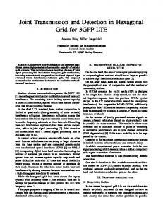
 Fig. 1.





        













 



       





 

 

       

 Block diagram of a MIMO-OFDMA LTE downlink.

[14]. There have been extensive work on the implementation

II. S YSTEM AND C HANNEL M ODELS

of the MIMO detection either with minimum mean square

The MIMO-OFDMA LTE system is a parallel of single-

error-successive interference cancellation (MMSE-SIC) [15],

input single-output OFDMA (SISO-OFDMA) where blocks

vertical-Bell Laboratories layered space-time (V-BLAST) [16]

of K data symbols are mapped onto the spatial multiplexing

or Maximum Likelihood (ML) receivers [17]-[22]. However,

(SM) module followed by the data mapping and inverse fast

while the formers usually provide an inferior performance,

Fourier transform (IFFT) operations, as shown in Figure 1.

the latter demandingly requires a large silicon complexity.

Note that we do not consider MIMO encoding (e.g., space-

Thus, finding a reasonable trade-off between an implementable

time coding) in this work. The data mapping operation is

architecture of the MIMO detector and a near ML performance

used for subcarrier mapping (e.g., distributed or localized

is always a motivation. We therefore extend our studies to the

mapping in multiple access [4]). Reversed operations are

implementation possibility of the proposed detector and then

carried out at the receiver, which are then followed by the

provide references for the possible real silicon implementation.

signal detection and MIMO processing. Assume that there

The rest of the paper is structured as follows. Section II describes the system and channel models. The signal detection algorithm is designed and discussed in Section III. Section IV studies the implementation possibility of the proposed detector. Section V provides simulation results and some concluding remarks are provided in Section VI. Notation: Bold-face upper (lower) letters denote matrices (column vectors); (·)∗ , (·)T and (·)H denote complex conjugation, transpose and Hermitian transpose, respectively; I is the identity matrix; E[·] denotes statistical expectation; Diag(x) denotes a matrix with vector x being its diagonal; N (µ, σ 2 )

denotes Gaussian distribution with mean µ and variance σ 2 ; δn,n� denotes Kronecker delta; J0 (·) denotes zero-order Bessel function of the first kind; | · | denotes absolute value; and � · � denotes Frobenius norm.

are K transmit antennas and N receive antennas. Let P and Q denote the number of subcarriers used in one orthogonal frequency division multiplexing (OFDM) symbol for the user of interest and the size of the IFFT, respectively. We denote sP,k = [s1,k , s2,k , · · · , sP,k ]T

(1)

as the transmitted signal vector from the kth transmit antenna. For convenience, it is assumed that E[sp,k s∗p,k ] = 1 for 1 ≤ p ≤ P, 1 ≤ k ≤ K.

Assuming that the guard interval (i.e., cyclic prefix (CP))

is longer than the maximum channel span, the received signal vector after removing CP and taking fast Fourier transform (FFT) at the nth receive antenna can be written as rP,n

� =

[r1,n , r2,n , · · · , rP,n ]T K � Diag(hn,k )sP,k + wn k=1

2011, © Copyright by authors, Published under agreement with IARIA - www.iaria.org

(2) (3)

International Journal on Advances in Telecommunications, vol 4 no 1 & 2, year 2011, http://www.iariajournals.org/telecommunications/

36 where hn,k = [hn,k (i1 ), hn,k (i2 ), · · · , hn,k (iP )]T is the

during one OFDM symbol interval. The maximum chan-

frequency-domain channel vector from the kth transmit an-

nel impulse span is also assumed to be within the guard

tenna to the nth receive antenna and wn is a zero-mean

interval. For convenience, let τl = lTs , Tb = T + Tg

2 complex Gaussian vector with variance σw . Here, ip = P(p)

where Ts = T /Q. Here, T , Tb and Tg denote the useful

where P(·) is the subcarrier mapping function that maps a

OFDM symbol interval, the whole OFDM symbol interval

data symbol onto one of the Q subcarriers. Obviously, ip

and the guard interval, respectively. Then, the channel impulse

is obtained depending on the subcarrier mapping pattern and

vector at each (OFDM symbol) time index n, denoted by

ip ∈ {1, 2, · · · , Q}. Note that

g(t) = [g0 (t), g1 (t), ..., gL−1 (t)]T , can represent the discrete

hn,k (ip ) =

L �

gn,k (l)e−

CIR. The autocorrelation function of gl (t) = g(lTs , tTb ) is

2πj Q (l−1)(ip −1)

expressed as

l=1

where gn,k (l) is the lth tap of the fading channel from kth transmit antenna to the nth receive antenna and L is the number of paths. We can rewrite the received signal for each subcarrier as follow

E{gl (t)gl∗� (t� )} = σl2 J0 (2πfD (t − t� )Tb )δl,l� ,

where fD is the maximum Doppler frequency and σl2 is the normalized average power of each propagation tap with L−1 �

(4)

rp,N = H(ip )sp,K + wp

(8)

σl2 = 1.

(9)

l=0

where rp,N = [rp,1 , rp,2 , ..., rp,N ]T , p = 0, 1, ..., P − 1, is

An typical urban (TU) power delay profile [23] is used to

N receive antennas. sp,K = [sp,1 , sp,2 , ..., sp,K ]T is the data

model {σl2 }.

the signal vector at the ip th subcarrier received through the symbol vector at the ip th subcarrier transmitted through K transmit antennas. wp is also the complex Gaussian noise vector. H(ip ) is the frequency-domain channel matrix at the ip th subcarrier given as  h1,1 (ip )   h2,1 (ip )  H(ip ) =  ..  . 

h1,2 (ip )

···

h1,K (ip )

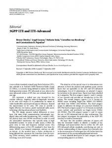
2) Spatial Channel Model: SCM was proposed by the

3GPP for both link- and system-level simulations. The 3GPP SCM emulates the double-directional and clustering effects of small scale fading mechanisms in a variety of environments, such as suburban macrocell, urban macrocell, and urban



    . (5)  

microcell. It considers N clusters of scatterers. A cluster

We assume that the channel is unchanged during one OFDM

given in Figure 2, where only one cluster of scatterers is

symbol interval and gn,k (l) is independent and has identical

shown as an example. Here, θv is the angle of the mobile

Gaussian distribution gn,k (l) ∼ N (0, σl2 ). Here, σl2 is the

station (MS) velocity vector with respect to the MS broadside,

h2,2 (ip ) .. .

hN,1 (ip )

hN,2 (ip )

··· .. .

h2,K (ip ) .. .

···

hN,K (ip )

normalized average power of each propagation path with L−1 �

σl2 = 1.

(6)

l=0

Typical urban (TU) [23] and spatial channel model (SCM) [24] power delay profiles are used in this paper. 1) Typical Urban: We consider the time varying channel whose channel impulse response (CIR) is modeled by L propagation paths, g(τ, t) =

L−1 � l=0

can be considered as a resolvable path. Within a resolvable path (cluster), there are M subpaths which are regarded as the unresolvable rays. A simplified plot of the SCM is

θn,m,AoD is the absolute angle of departure (AoD) for the mth (m = 1, ..., M ) subpath of the nth (n = 1, ..., N ) path at the base station (BS) with respect to the BS broadside, and θn,m,AoA is the absolute angle of arrival (AoA) for the mth subpath of the nth path at the MS with respect to the MS broadside. Details of the generation of SCM simulation parameters can be found in [24]. III. S IGNAL D ETECTION

γl (t)δ(τ − τl ).

(7)

Assume that the channel is a wide-sense stationary uncorrelated scattering (WSSUS) Rayleigh fading and unchanged

For convenience, the indices in (4) are omitted. The N × 1

received signal vector rp,N , now denoted by r, is given by r = Hs + w,

2011, © Copyright by authors, Published under agreement with IARIA - www.iaria.org

(10)

International Journal on Advances in Telecommunications, vol 4 no 1 & 2, year 2011, http://www.iariajournals.org/telecommunications/

37 



 

'  



'  

T T   





T 

 



Fig. 2.

BS and MS angle parameters in the 3GPP SCM with one cluster of scatterers [24].

where H, s, and w are the N × K channel matrix, the K × 1 transmitted signal vector, and the N × 1 noise vector, respectively. Let S denote the signal alphabet for symbols, i.e.,

sk ∈ S, where sk denotes the kth element of s, and its size is denoted by M , i.e., M = |S|.

Pr(bi = −1|r)

We consider two conventional detection approaches: ML

(13)

sk ∈ S, ∀k, is not imposed. Using the orthogonality principle, the MMSE estimator for s can be found as Wmmse

=

arg max f (r|s)

=

arg min ||r − Hs||2 .

s∈S K s∈S K

We can show that E[rrH ]

(11)

H

E[rs ]

To identify the ML vector, an exhaustive search is required. Because the number of candidate vectors for s is M K , the If the a priori probability of s is available, the maximum a posteriori (MAP) sequence detection can be formulated. Suppose that b is a bit-level symbol vector representation of s. The elements of b are binary and the size of b is (K log2 M ) × 1. With the a priori probability of b, the MAP vector (at the bit-level) becomes

arg max Pr(b|r)

=

arg max f (r|b) Pr(b),

b b

b∈Bi+

2 HHH + σw I

=

H.

2 −1 Wmmse = (HHH + σw I) H

and ˆsmmse

=

H Wmmse r

=

2 −1 HH (HHH + σw I) r.

(15)

B. Proposed Detector of the channel matrix as H = QR, where Q is unitary and

(12)

the a posteriori probability of each bit can be found by �

=

(14)

We assume that N ≥ K and consider the QR factorization

where Pr(b) denotes the a priori probability of b. In addition, marginalization as

arg min E[||s − WH r||2 ] � WH �−1 E[rr ] E[rsH ].

It follows that

complexity grows exponentially with K.

=

= =

vector that maximizes the likelihood function as follows:

=

Pr(b|r),

b∈Bi−

2) MMSE Detection: It is easy to perform the (linear)

1) ML Detection: The ML detection finds the data symbol

Pr(bi = +1|r)

�

where Bi± = {[b1 b2 . . . bK¯ ]T | bi = ±1, bm ∈ ¯ = K log2 M . {+1, −1}, ∀m �= i} and K

and MMSE.

bmap

=

MMSE detection if the constraint on the symbol vector,

A. Conventional Detectors

sml



G 

G 

: 

T

:  T   

R is upper triangle. We have x = QH r = Rs + QH w.

(16)

Since the statistical properties of QH w are identical to that of w, QH w will be denoted by w. If N = K, there is no

Pr(b|r)

zero rows in R, otherwise the last N − K rows would be zero. Thus, the last N − K elements of x would be ignored

2011, © Copyright by authors, Published under agreement with IARIA - www.iaria.org

International Journal on Advances in Telecommunications, vol 4 no 1 & 2, year 2011, http://www.iariajournals.org/telecommunications/

38 for the detection if N > K. Accordingly, the first K rows AS3) The list of candidates of s2 , denoted by S2 , can be of R would be considered. If there is no risk of confusion, hereafter, we assume that the sizes of x, R, and w are K × 1, K × K, and K × 1, respectively.

The complexity of the conventional LR based detector can

converted from C2 . For convenience, denote S2 = (1)

(2)

AS4) Once S2 is available, the LR-based detection of s1 can be carried out with SIC, i.e.,

grows significantly with the number of basis vectors. To avoid this problem, we propose an LRLD based detection algorithm, which breaks a high dimensional MIMO detection

(Q)

{˜s2 , ˜s2 , · · · , ˜s2 }.

(q)

(q)

˜1 = LRDet(x1 − R3˜s2 ), c (q)

where ˜s2 (q) ˜s1

is the qth decision vector of s2 from list S2 . (q)

˜1 in denote the signal vector corresponding to c problem into multiple lower dimensional MIMO sub-detection AS5) Let (q) T (q) T T (q) the LR domain and ˜s = [(˜s1 ) (˜s2 ) ] , the final problems. To perform the proposed LRLD based detection, we consider the partition of x as follows: � � � �� � � � x1 R1 R3 s1 w1 + , = x2 0 R2 s2 w2

decision of s is found as ˜s = arg

(17)

where xi , si , and wi denote the Ki × 1 ith subvectors of x,

s, and w, i = 1, 2, respectively. Note that K1 + K2 = K. From (17), we can have two lower dimensional MIMO subdetection problems to detect s1 and s2 . It is straightforward to extend the partition into more than two groups. However, for the sake of simplicity, we only consider the partition into

min

q=1,2,··· ,Q

� �2 � � �x − R˜s(q) � .

Softbit Generation: As we are using turbo code for channel coding, its inputs should be soft bits. The probability of the qth candidate ˆs(q) in the list can be found as � � 1 (q) (q) 2 P (ˆs ) = CQ exp − 2 ||x − Rˆs || , σw

(18)

where CQ is the normalization constant, which is given by 1 � �. CQ = � 1 s(q) ||2 q=1,··· ,Q exp − σ 2 ||x − Rˆ w

two groups as in (17). In the proposed LRLD based detection, the sub-detection of s2 is carried out first using the LR based detector. Then, a list of candidate vectors of s2 is generated. With the list of s2 , the sub-detection of s1 is performed with the LR based detector. The candidate vector in the list is used for the SIC to mitigate the interference from s2 . The algorithm steps (AS) of the proposed LRLD based detector is summarized as follows. AS1) The LR based detection of s2 is performed with the received signal x2 , i.e.,

Note that

�

P (ˆs(q) ) = 1.

(19)

q=1,··· ,Q

ˆ (q) is a bit-level symbol vector representation Suppose that b ˆ (q) ) where M(·) denotes the mapping of ˆs(q) , i.e., ˆs(q) = M(b ˆ (q) are binary and the size of b ˆ (q) is rule. The elements of b ¯ ×1 where K ¯ = K log2 M . Correspondingly, the probability K ˆ (q) can be written as of b � � 1 (q) (q) 2 ˆ ˆ P (b ) = CQ exp − 2 ||x − RM(b )|| , σw

(20)

LR domain. Note that there is no interference from s1 in

The soft log-likelihood ratio (LLR) value of the ith bit bi ¯ can then be obtained as (i = 1, 2, · · · , K) � ˆ (q) ) ˆ (q) ∈B+ P (b b i Λ(bi ) = log � , (21) ˆ (q) ) ˆ (q) ∈B− P (b b

detecting s2 .

{+1, −1}, ∀m �= i}.

˜2 = LRDet(x2 ), c where LRDet(·) is the function of the LR detection operation (see Appendix A for details of the LR detection), ˜2 is the estimated vector of s2 in the corresponding and c

AS2) A list of candidate vectors in the lattice-reduced domain is generated by

i

where Bi± = {[b1 b2 . . . bK¯ ]T |

bi = ±1, bm ∈

IV. I MPLEMENTATION S TUDY OF THE P ROPOSED D ETECTOR

C2 = List(˜ c2 ),

In this section, we study the implementation possibility of

where List is a function that chooses the Q closest vectors

the proposed LRLD detector. Note that some details of the

˜2 (1 ≤ Q ≤ M K2 ) in the LR domain. The details of to c

proposed detector and definition of certain parameters, e.g.,

the list generation is discussed in Appendix B.

α, β, are presented in Appendix A and B.

2011, © Copyright by authors, Published under agreement with IARIA - www.iaria.org

International Journal on Advances in Telecommunications, vol 4 no 1 & 2, year 2011, http://www.iariajournals.org/telecommunications/

39 (q)

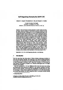
A. Detector Structure For convenience, we outline the implementation steps (IS)

processing, in which all operations need to be carried out only

H = QR, where R=

�

when there is a new channel update. All steps from IS1) to

R1

R3

0

R2

�

IS3) belong to this type. Detection Processing: This can be referred to as symbol-rate

.

processing. This type of processing includes all operations that

IS2) Gaussian lattice reduction:

are carried out after each received signal vector arrives. In our proposed detector, the received data will be processed in a

¯ 1 = R1 U 1 , R

first in first out (FIFO) manner. The FIFO buffer is used to

¯ 2 = R2 U 2 . R

bridge the latency incurred among the received signals. All steps from IS4) to IS6) belong to this type.

IS3) MMSE filtering weight matrices: 2 2 2 −1 2 W1 = (R1 RH R1 U−H 1 α Es + |α| σw I) 1 α Es , 2 2 2 −1 2 W2 = (R2 RH R2 U−H 2 α Es + |α| σw I) 2 α Es .

x2

=

describe each major operation next. Some operations such as

not a big issue in the hardware implementation, we assume that

= Rs + w, �

detector with respect to hardware implementation. We will

straightforward and thus ignored. Since memory is nowadays

x = QH r

�

Figure 3 shows a high-level structure of the proposed

unitary transformation, shifting/scaling and final decision are

IS4) Unitary transformation:

x1

The implementation operations can be classified into two Pre-processing: This is often referred to as channel-rate

IS1) QR decomposition:

�

(q)

types: Pre-processing and detection processing.

required for the proposed detector as follows.

or

(q)

where s2 = (U2 c2 − β1)/α and c2 ∈ C2 .

R1

R3

0

R2

��

a certain amount of memory is available wherever needed.

s1 s2

�

+

�

w1 w2

�

B. Pre-Processing .

IS5) Scaling/shifting:

In our proposed detector, there are three dominant components in the pre-processing stage – QR decomposition, Gaussian lattice reduction and matrix inversion operations. It

d2 = αx2 + βR2 1,

is always desirable to have a low latency in preprocessing

b2 = αs2 + β1,

the channel matrices. Thus, selection of algorithm to be

(q) d1

= α(x1 −

(q) R3ˆs2 )

+ βR1 1,

decide the real silicon complexity. We will consider each

b1 = αs1 + β1. IS6) LR based list detection: This step includes three stages: – one MMSE filtering operation to estimate c2 (i.e., signal vector s2 in the LR domain): ˜2 = W2H (d2 − βR2 1) + U−1 c 2 β1 = αW2H x2 + U−1 2 β1.

– sorting and storing the list of c2 (of length Q): � C2 = {c2 � ||˜ c2 − c2 || < r(Q)}.

– Q parallel MMSE filtering operations to estimate c1 with respect to each candidate of the list of c2 : (q)

implemented for each of the three above operations may well

(q)

˜1 = αW1H (x1 − R3ˆs2 ) + U−1 c 1 β1,

operation in details next. 1) QR Decomposition: As shown in [25], QR decomposition is preferred to Cholesky decomposition due to the numerical stability. In our detection algorithm, although the QR operation is required only once for each channel update, it still provides a significant load of computations as the operation is carried out to the channel matrix of full size. We therefore study different algorithms in the literature for the QR decomposition. Gram-Schmidt: The Gram-Schmidt (GS) procedure finds the QR decomposition of a matrix H such that H = QR, where Q is unitary and R is upper triangular. An obvious drawback of

2011, © Copyright by authors, Published under agreement with IARIA - www.iaria.org

International Journal on Advances in Telecommunications, vol 4 no 1 & 2, year 2011, http://www.iariajournals.org/telecommunications/

40 Pre-processing

H

QR Decomposition

Q, R

QR Memory

Ri

Q

MMSE Filter Weight Memory

Matrix Inversion

W2

Detection Processing

r

W1 LR based list detector

uQH Scaling /Shifting

x Data FIFO

LR look-up table of c 2

Ui

Gaussian LR

d2

MMSE filtering ( s 2 )

~c 2

x2

List Sorting & Memory

x1

MMSE filtering ( s1 ) LR based List LR based List

Final Decision

sˆ

(q) _ {R 3sˆ 2 }

Scaling /Shifting

+

Fig. 3.

d1( q )

High-level structure diagram of the implementation of the proposed LR based list detector.

the GS algorithm is the fact that it requires costly square-

point version of the GS algorithm is bounded by the product

root and division operations and that the overall computational

of condition number κ(H) of matrix H and machine precision

complexity is high. Thus, a modified version of the GS is

ε, as follows

presented (see [26]). The details of the modified GS are discussed in [27], [28]. The corresponding algorithm proceeds

�o =� I − QH Q � ≤ ζ(K) × ε × κ(H),

as follows. Gram-Schmidt algorithm:

where ζ(K) is a low degree polynomial in K depending only

1) initialize: Q = H, R = 0

on details of computer arithmetic. This implies that for a well-

2) for k = 1 to � K 3) [R]k,k = qH k qk

conditioned matrix, fixed-point architecture for the GS is still

4)

qk = qk /[R]k,k

5)

for i = k + 1 to K

very far from orthogonal. Thus, we can consider the numer-

6)

[R]k,i =

7)

qi = qi − [R]k,i qk

8)

qH k qi

end for

9) end for

accurate to the integer multiples of the machine precision ε. However, for ill-conditioned matrices, the computed Q can be ically more favorable scheme, Householder Transformation, which is based on unitary transformation. Householder Transformation: The use of unitary transformations instead of the conven-

Generally, the GS is accurate to the floating-point precision.

tional methods is to alleviate the numerical problem such as

For fixed-point arithmetic, the problem of quantization and

requirement of high number precision, i.e., large silicon area in

round-off errors is not ignorable and therefore there is loss

fixed-point very-large-scale integration (VLSI) implementation

in accuracy (e.g., loss in the orthogonality of Q) [27]. It was

is required. The reason for this more favorable behavior is

shown in [29] that the orthogonalization error (�o ) in fixed-

that unitary transformations do not alter the length of a vector

2011, © Copyright by authors, Published under agreement with IARIA - www.iaria.org

International Journal on Advances in Telecommunications, vol 4 no 1 & 2, year 2011, http://www.iariajournals.org/telecommunications/

41 and thus cannot lead to an excessive increase in dynamic range or to an enhancement of quantization noise. Two typi-

these matrices of size 2 × 2 only. Thus, this basis-2 LR

can be carried out using the simple Gaussian method. We

cal algorithms using unitary transformations are Householder

can limit the maximum number of iterations in this Gaussian

Transformation and Givens Rotation. For illustrative purpose,

lattice reduction algorithm to a small number (e.g., 2 iterations

we overview the Householder Reflection algorithm only.

is reasonable) while keeping the overall performance almost

The Householder Transformation algorithm recursively applies a sequence of unitary transformations

QH i

to matrix H

as follows:

where R

maximum number of iterations to T , and the Gaussian LR algorithm is summarized as follows.

R (1)

the same. For the implementation purpose, we can fix the

=

(k+1)

=

(k) QH , kR

H. Each transformation will eliminate

more subdiagonal entries until finally R = R(K−1) = H H QH is readily obtained K−1 · · · Q1 H. The unitary matrix Q

from

1) Input (b�1 , b2 , T )� � 0 1 1 2) Set J = and U = 1 0 0 3) i = 0

6)

if ||b1 || > ||b2 ||

swap b1 and b2 , and U = UJ

The algorithm can be described in details as follows.

7)

end if

Householder Transformation algorithm:

8)

1) initialize: Q

9)

if | < b2 , b1 > | > 1/2 tˆ = � �

(0)

= I, R

(1)

=H

||b1 ||

2) for k = 1 to K − 1

10)

4)

11)

end if

12)

i=i+1

3)

5) 6) 7)

¯ k = rk + � rk � 1 q H ¯ k = I − 2 q¯ k q¯ k2 Q �¯ q � k � � Ik−1 0 Pk = ¯k 0 Q [R]H k+1 (k) Q

= Pk R

= Pk Q

1

�

4) do 5)

H QH = QH K−1 · · · Q1 .

0

b2 = b2 − tˆb1 and U = U

�

1 0

−t 1

�

13) while (||b1 || < ||b2 ||)&&(i ≤ T ) 14) return (b1 , b2 , U)

(k)

(k−1)

In the worst case where the Gaussian LR algorithm runs until

8) end for

the maximum iteration i = T , the number of CMs required

9) QH = Q(K−1)

for the Gaussian LR is 4T . Six words of memory are required

We compare the complexity of the two methods in Table

to store data of the unimodular matrix at the output.

I. The Householder Reflection algorithm provides a slightly

3) Matrix Inversion: In our proposed detector, the dominant

lower number of complex multiplications (CMs), divisions

complexity component in obtaining the MMSE filtering weight

and square root operations compared to the Gram-Schmidt

2 matrices is the matrix inversion operations, (R1 RH 1 α Es +

algorithm. In addition, for fixed-point implementation, the

2 −1 2 2 2 −1 |α|2 σw I) and (R2 RH . Fortunately, the 2 α Es + |α| σw I)

Householder Reflection algorithm is supposed to be more stable. 2

Note that (K + K(K + 1)/2) words of memory are 2

required to store matrices Q and R at the output of the QR decomposition operation. 2) Lattice Reduction Using Gaussian Method: In the proposed LR based list detector, the LR is applied to the subchannel matrix R1 and R2 . For convenience, we consider 2 The

term ‘word of memory’ is referred to the amount of memory required to store one complex number. The number of bits in one word may vary depending on the dynamic range of the observing data. Thus, throughout the section, we use ‘word’ as a unit of memory.

fact that the size of these submatrices to be inverted is reasonably small leads to a reasonably�low load of computations. For � r1,1 r1,2 example, a 2 × 2 matrix R = can be simply r2,1 r2,2 inverted using adjoint method � � r2,2 −r2,1 1 −1 R = , r1,2 r2,1 − r1,1 r1,1 −r1,2 r1,1 which requires 1 division and 6 CMs. In a general case of matrix H of size K ×K, the complexity

of inversion operation may vary depending on implementation method. We overview some typical methods:

2011, © Copyright by authors, Published under agreement with IARIA - www.iaria.org

International Journal on Advances in Telecommunications, vol 4 no 1 & 2, year 2011, http://www.iariajournals.org/telecommunications/

42 TABLE I C OMPLEXITY COMPARISON OF THE TWO METHODS : G RAM -S CHMIDT (GS) AND H OUSEHOLDER R EFLECTION (HR)

Algorithm

Division

Square root

GS

K

K

HR

K−1

K−1

Complex multiplications (CMs) 2K 2 + 2

a) Adjoint Method:

2

�K

�K−1 k=1

k=1

CMs with K = 4 80

K(K − k)

78

(K − k + 1)2

of the quantization noise and thus requires a high fixed point H−1 =

precision.

adj(H) . det(H)

A VLSI architecture has therefore been proposed in [28] to

Unfortunately, for the matrix inversion using adjoint method,

deal with numerical problems for fixed-point implementation.

there is no generic expression for the number of CMs as it

It was based on the QR decomposition with modified Gram-

depends heavily on the dimension K. However, the approxi-

Schmidt algorithm. The results showed that for typical 4 × 4

mated number of CMs can be of up to scale in 2

K

as [30]

Cm ≈ a2K + K 2 + K. b) LR Decomposition: Matrix H is decomposed into a

MIMO channel matrices, the architecture was able to achieve a clock rate of 277 MHz with a latency of 18 time units and area of 72K gates using 0.18 − µm CMOS technology, which

is impressive compared to previously known architectures. In

lower-triangular matrix L and a upper-triangular matrix R,

other direction, the architecture can be designed focusing on

i.e., H

reducing number of matrix inversions, which is well-suited to

−1

=R

−1

L

−1

. The algorithm is as follows

the systems with multiple channels to be processed such as

1) Initiate L = H, R = I

MIMO-OFDM systems [31], [30].

2) For i = 1 to K 3)

For j = 1 to K

4)

[R]j,i = [L]j,i −

5) 6)

[L]j,i =

[R]j,i [R]i,i

�j−1

k=1 [L]j,k [R]k,j

end for

7) end for The number of CMs for matrix inversion using LR decomposition is 4(K 3 − K)/3.

c) QR Decomposition: Matrix H can be inverted using

QR decomposition as H−1 = R−1 QH . If Gram-Schmidt algorithm is used for QR decomposition, the total number of CMs required for matrix inversion is (9K 3 + 10K 2 − K)/6.

In general, a major concern with matrix inversion algorithms

is the need for a high number precision which gives rise to a large silicon area in fixed-point VLSI implementations. The two main reasons for these numerical requirements are: i) the use of costly operation such as square root and divisions, which leads to a significant increase of the dynamic range for some intermediate variables; and ii) the desire to replace repeated divisions by multiplications with the corresponding inverse in order to reduce the number of costly operations. Unfortunately, multiplications often results in an enhancement

C. Detection Processing This is where all operations are carried out when a new set of received signal symbols arrives. The resources required for the detection processing is in fact much less compared to the preprocessing stage. In addition, the hardware for preprocessing can be conveniently reused for the detection processing. As a result, the latency in the detection processing is reasonably low. Two operations will be discussed in this section: List sorting in the lattice domain and MMSE filtering to find the estimates of s1 and s2 . 1) List Sorting in LR Domain: The list of candidate vectors in the LR domain is formed by � C2 = {c2 � ||˜ c2 − c2 || < r(Q)}.

The problem is that the alphabet of signal in LR domain (c2 ) varies depending on channel. For example, while the alphabet of s2 is known, that of c2 = U−1 2 (αs2 + β1) depends on U2 . However, with Gaussian reduction method, U2 has always a form of U2 =

�

1

t

0

1

�

,

2011, © Copyright by authors, Published under agreement with IARIA - www.iaria.org

International Journal on Advances in Telecommunications, vol 4 no 1 & 2, year 2011, http://www.iariajournals.org/telecommunications/

43 (q)

4. Filtering operation for x1

>u2 @i

can be carried out similarly.

Due to different dynamic ranges, variables can be represented

>x2 @i D >W2 @ j, i

by different numbers of bits (e.g., n bits for x2 whereas m n bits

m bits

u

>~c2 @ j

+

+ m bits

m bits

bits for W2 ). It is expected that m > n as entries of W2 has a larger dynamic range, thus they should be presented with considerable number of bits for the accurate fixed-point implementation. Memory-wise, there are 2Q words required to store the

Fig. 4. Block diagram of the linear filtering operation: Inputs are x2 , α, ˜2 . W2 and u2 while output is c

where t is an integer. As the maximum number of iterations in the Gaussian LR algorithm is limited to T = 2 or 3 only, we can easily obtain a known set of t (and accordingly U2 ). Thus, a look-up table can be formed for the alphabet of c2 . This look-up table is formed in the pre-processing stage after the Gaussian LR algorithm is carried out to subchannel matrix R2 . Memory is required to store this pre-calculated data. For example, it requires T M words of memory to store the alphabet of c2 , where M is the size of alphabet of s2 . In addition, 2Q words are required for storing C2 .

˜2 , · · · , c ˜Q }. outputs {˜ c1 , c D. Fixed-Point Considerations A critical issue in fixed-point arithmetic is the difference in dynamic ranges of variables. Number of integer and fractional bits for each variable should be carefully determined to avoid overflows and, at the same time, not to waste hardware resources. For example, entries of channel matrix H is usually assumed to be Gaussian distributed, thus has a infinite dynamic range. To deal with this problem, two common approaches can be employed: •

2) MMSE filtering: This is a matrix-multiplication based

rounding errors during fixed point arithmetic operations)

applied to received signal vector x2 : ˜2 = c

resenting H to ensure that overflows occur only rarely. At the same time, the round-off error (i.e., accumulation of

operation. One MMSE filtering operation to estimate c2 is

αW2H x2

A sufficiently large number of integer bits is used for rep-

should be purely due to loss in fractional precision. In this case, it is shown in [27] that the error variance varies only

+ u2 ,

with the number of fractional bits, η, in the form:

where u2 = U−1 2 β1. Q times of same operation are applied

σe2 = 2−2η /3.

to received signal vector x1 : (q)

(q)

˜1 = αW1H x ¯ 1 + u1 , c (q)

¯1 where u1 = U−1 1 β1 and x

(22) (q)

= x1 − R3ˆs2 . Note that Q

operations in (22) can be carried out in parallel (see Figure 3). The parallel structure often allows low latency and high

•

Automatic gain control adjusts the data of H to the available number of integer bits with an appropriate scaling factor γ in which the new channel matrix become ¯ = γH. γ can be chosen as H γ=

throughput. The most complex steps can then be processed in a single cycle, however, at the expense of large silicon area. In addition, with parallel structure, memories need to be implemented based on register files for sufficient access bandwidth. Thus, trade-off between latency/throughput and silicon area needs to be considered. The weight matrices W1 and W2 are pre-calculated and stored in the pre-processing stage. Note that only 8 words

1 . max |[H]i,j |

Depending on hardware resources, each approach can be applied. However, practical systems tend to compromise between the two approaches. V. S IMULATION R ESULTS We run simulations for MIMO-OFDMA LTE downlink system with parameters being given in Table II.

of memory are needed for this storage requirement. A simple

Figures 5 and 6 show bit error rate (BER) performance

VLSI architecture for MMSE filtering of x2 is shown in Figure

of different detectors for TU and SCM channels. 4-QAM is

2011, © Copyright by authors, Published under agreement with IARIA - www.iaria.org

International Journal on Advances in Telecommunications, vol 4 no 1 & 2, year 2011, http://www.iariajournals.org/telecommunications/

44 TABLE II S IMULATION PARAMETERS Value

Center Frequency

3.5GHz

Bandwidth

10MHz

Subcarrier Spacing

15kHz

FFT size

1024

−1

10

−2

10 BER

Parameter

Number of usable subcarriers

601

Cyclic Prefix (CP)

FFT size / 8

Channel Model & Velocity

TU-30km/h and SCM-3km/h

Modulation

16-QAM, Gray Mapping

Channel Coding

Turbo Coding, Code Rate 1/2

Channel Estimation

Ideal

Data Mapping

Localized Subcarrier Pattern

−3

10

LR−based MMSE (LLL)

−4

10

Proposed LRLD Sphere ML

−5

10

4

4.5

5

5.5

6

6.5 Eb/N0 (dB)

7

7.5

8

8.5

9

Fig. 7. BER performance comparison of different detectors with 16QAM modulation and TU channel (receiver velocity of 30kmh.)

OFDMA−4QAM−Rate1/2−TU−30kmh

−1

OFDMA−16QAM−Rate1/2−TU−30kmh

0

10

10

OFDMA−16QAM−Rate1/2−SCM−3kmh

0

10

−2

10

−1

10 −3

BER

10

−2

10 −4

BER

10

−5

−3

10

LR based MMSE (LLL)

10

−4

Proposed LRLD (Q = 6)

10

Sphere ML

LR based MMSE (LLL) Proposed LRLD (Q=12)

−6

10

0

−5

0.5

1

1.5

2

2.5 Eb/N0 (dB)

3

3.5

4

4.5

5

Sphere ML

10

−6

10

Fig. 5. BER performance comparison of different detectors with 4QAM modulation and TU channel (receiver velocity of 30kmh.)

8

9

10

11

12 Eb/N0 (dB)

13

14

15

16

Fig. 8. BER performance comparison of different detectors with 16QAM modulation and SCM channel (receiver velocity of 3kmh.) OFDMA−4QAM−Rate1/2−SCM−3kmh

0

10

LR based MMSE (LLL) Proposed LRLD (Q=6) Sphere ML

−1

used for modulation. We compare the proposed LRLD based

10

detector with the conventional LR based Minimum Mean −2

Square Error (MMSE) detector that uses LenstraLenstraLovsz

BER

10

(LLL) algorithm [32] and the optimal sphere ML detector.

−3

10

It can be seen that the proposed detector provides a near ML performance and outperform the conventional LR based

−4

10

MMSE detector. The same behaviour is observed with 16−5

10

QAM modulation in Figures 7 and 8.

−6

10

4

5

6

7

8 Eb/N0 (dB)

9

10

11

12

Complexity comparison: To fully examine the complexity of different detection methods, simulation is considered and results are shown in Figure 9 where the estimated flops using

Fig. 6. BER performance comparison of different detectors 4QAM modulation and SCM channel (receiver velocity of 3kmh.)

MATLAB execution time were obtained over all operations for each detector under the same environment. The execution time

2011, © Copyright by authors, Published under agreement with IARIA - www.iaria.org

  

International Journal on Advances in Telecommunications, vol 4 no 1 & 2, year 2011, http://www.iariajournals.org/telecommunications/

TABLE III S IGNALS AND PARAMETERS FOR THE LR- BASED DETECTION









   

Steps AS4)



y

AS1)







x2 (q)

x 1 − R2 ˆ s2

A

z

R2

s2

R1

s1

˜ c

Ki

˜2 c

K2

(q)

K1

˜1 c

respectively. For example, for M -QAM, if M = 22m , we have







45

S = {s = a + jb|a, b ∈ {±A, ±3A, . . . , ±(2m − 1)A}}, 







Fig. 9.

 









Complexity comparison.

where A =

�

(3Es /2(M − 1)) and Es = E[|s|2 ] denotes the

symbol energy. Thus, α = 1/(2A) and β = ((2m − 1)/2)(1 + j). Note that the pair of α and β is not uniquely decided.

Consider the MIMO detection with the following signal: is averaged over hundreds of thousands of channel realizations.

(23)

Note that Schnorr-Euchner algorithm [33] is used for sphere

y = Az + v,

ML detector. The LLL-reduced algorithm with reduction factor

where A is a MIMO channel matrix, z ∈ S Ki is the signal

δ = 3/4 [32] is chosen for the LR based MMSE-SIC detector. No limitation on the number of iterations is imposed for any LR algorithm. The proposed LRLD based detector clearly requires the lowest number of flops. We can also see that the number of flops of the proposed detector is slightly higher than half of that of the LR based MMSE-SIC detector where the LLL-reduced algorithm is used. VI. C ONCLUSION An efficient signal detector based on two techniques, namely LR and LD, has been investigated in this paper for the MIMO-OFDMA LTE downlink systems. By generating the list in LR domain, a more reliable list detection is obtained to facilitate SIC detection. As a result, the proposed detector

vector, and v is a zero-mean Gaussian noise with E[vvH ] = 2 σw I. We scale and shift y as

d = αy + βA1 = A(αz + β1) + αv = Ab + αv,

(24)

where 1 = [1 1 . . . 1]T , and b = αz + β1 ∈ CKi . Let ¯ = AU where U is a unimodular matrix. Using any LR A algorithm including LLL algorithm [32], we can find U that ¯ shorter. It follows that makes the column vectors of A ¯ + αv, d = AUU−1 b + αv = Ac

(25)

where c = U−1 b. The MMSE filter to estimate c is given by ¯ − (c − c ¯)||2 ] Wmmse = min E[||WH (d − d) W

outperforms conventional LR based detectors and provides a

2 −1 = (AAH α2 Es + |α|2 σw I) AU−H α2 Es , (26)

near ML performance with significantly reduced complexity.

¯ = E[d] = βA1, c ¯ = E[c] = U−1 β1, and Cov(c) = where d

The implementation possibility was then studied to provide

|α|2 U−1 U−H Es . The estimate of c is given by:

references for the real silicon implementation. A PPENDIX A LR BASED S IGNAL D ETECTION We describe the LR based detection that is used in Steps AS1 and AS4. Let C denote the set of complex integers or Gaussian integers, C = Z + jZ, where Z denotes the set of √ integers and j = −1. We assume that {αs + β|s ∈ S} ⊆ C, where α and β are the scaling and shifting coefficients,

H ¯ ˜=c ¯ + Wmmse c (d − d).

In Table III, the signals and parameters for the LR based MMSE detection for each step are shown. A PPENDIX B L IST G ENERATION IN THE LR D OMAIN To avoid or mitigate the error propagation, the use of a list of candidate vectors of s2 in detecting s1 is crucial. Using the

2011, © Copyright by authors, Published under agreement with IARIA - www.iaria.org

International Journal on Advances in Telecommunications, vol 4 no 1 & 2, year 2011, http://www.iariajournals.org/telecommunications/

46 ML metric, we can find the candidate vectors in the list, S2 . Let

(1)

(2)

(M

||r − R2ˆs2 ||2 ≤ ||r − R2ˆs2 ||2 ≤ . . . ≤ ||r − R2ˆs2 where

(q) ˆs2

K2

) 2

|| ,

denotes the symbol vector that corresponds to the

qth largest likelihood. Therefore, an ideal list would be (1)

(2)

(Q)

S2 = {ˆs2 , ˆs2 , . . . , ˆs2 }.

(27)

a high computational complexity due to computing of R2 s2 for all s2 ∈ S

.

To avoid a high computational complexity, we can find

a suboptimal list in the LR domain with low complexity. Consider (24). According to Table III, let A = R2 , d = ¯ = AU, we αx2 + βA1, and b = αs2 + β1. Then, since A can see that the ML metric to construct the list is given by ¯ ||d − Ab|| = ||d − Ac||.

(28)

It is noteworthy that the metric on the right hand side in (28) is defined in the LR domain. Let ˜s2 be the signal vector in ˜2 and assume that ˜s2 is sufficiently S K2 corresponding to c (1) ¯ c2 . From this, the ML close to ˆs . Then, we can have d � A˜ 2

metric (ignoring a scaling factor) for constructing the list in the LR domain becomes

¯ ¯ c2 − Ac|| ¯ ||d − Ac|| = ||A˜ = ||˜ c2 − c||A (29) ¯ HA ¯, √ where ||x||A = xH Ax is a weighted norm. The list in the LR domain becomes

� C2 = {c � ||˜ c2 − c||A ¯ HA ¯ < rA ¯ (Q)},

(30)

where rA ¯ (Q) > 0 is the radius of an ellipsoid centered at ˜2 , which contains Q elements in the LR domain. If the c ¯ or the basis vectors in the LR domain column vectors of A H ¯ A ¯ becomes diagonal. Furthermore, if they are orthogonal, A ¯ HA ¯ ∝ I. Thus, for nearly orthogonal have the same norm, A basis vectors of almost equal norm, the list of c2 can be approximated as � C2 � {c � ||˜ c2 − c|| < r(Q)},

multiplications are required to generate C2 or S2 , we can use S2 as the list in the proposed detector to reduce computational

complexity. Note that the list generated in the LR domain is much more reliable than the list generated in the original domain (this list is different from S2 ).

However, this requires an exhaustive search, which results in K2

converted from C2 as in step AS3. Since no matrix-vector

(31)

˜2 , which where r(Q) > 0 is the radius of a sphere centered at c contains Q elements. Since the LR provides a set of nearly orthogonal basis vectors for the LR based detection, we can ¯ are nearly orthogonal with a a see that the column vectors in A two-basis system. Let S2 denotes the list in the original domain

R EFERENCES [1] H. X. Nguyen, “An efficient signal detection algorithm for 3GPP LTE downlink,” in Proc. IEEE International Conf. on Digital Telecommunications (ICDT 2010), Athens, Greece, Jun. 2010, pp. 77-81. [2] 3rd Generation Partnership Project (3GPP) TR 25.814, “Technical specification group radio access network: Physical layer aspects for Evolved UTRA,” http://www.3gpp.org/ftp/Specs/html-info/25814.htm. [3] H. Ekstrom, A. Furuskar, J. Karlsson, M. Meyer, S. Parkvall, J. Torsner, and M. Wahlqvist, “Technical solutions for the 3G Long-Term Evolution,” IEEE Commun. Mag., vol. 44, pp. 38-45, Mar. 2006. [4] H. G. Myung, J. Lim, and D. J. Goodman, “Single carrier FDMA for uplink wireless transmission,” IEEE Veh. Technol. Mag., vol. 1, pp. 3038, Sep. 2006. [5] G. J. Foschini, G. Golden, R. Valenzuela, and P. Wolniansky, “Simplified processing for wireless communication at high spectral efficiency,” IEEE J. Select. Areas Commun., no. 11, pp. 1841-1852, 1999. [6] W. J. Choi, R. Negi, and J. Cioffi, “Combined ML and DFE decoding fo the V-BLAST system,” in Proc. IEEE International Conf. Communications, New Orleans, LA, 2000, pp. 1243-1248. [7] J. Luo, K. Pattipati, P. Willett, and F. Hasegawa, “Near optimal multiuser detection in synchronous CDMA using probabilistic data association,” IEEE Commun. Lett., vol. 5, pp. 361-363, Sep. 2001. [8] D. Pham, K. R. Pattipati, P. K. Willett, and J. Luo “A generalized probabilistic data association detector for multiple antenna systems,” IEEE Commun. Lett., vol. 8, no. 4, April 2004. [9] J. Choi, “On the partial MAP detection with applications to MIMO channels,” IEEE Trans. Signal Proc., vol.53, pp.158-167, Jan. 2005. [10] D. J. Love, S. Hosur, A. Batra, and R. W. Heath, “Chase decoding for space-time codes,” in Proc. IEEE Vehicular Technology Conf., vol. 3, Nov. 2004, pp. 1663-1667. [11] D. W. Waters and J. R. Barry, “The Chase family of detection algorithms for multiple-input multiple-output channels,” IEEE Trans. Signal Proc., vol. 56, No. 2, pp. 739-747, February 2008. [12] H. Yao and G. W. Wornell, “Lattice-reduction-aided detectors for MIMO communication systems,” in Proc. IEEE Global Telecommunications Conf., Taiwan, Nov. 2002, pp. 424-428. [13] D. Wubben, R. Bohnke, V. Kuhn and K. -D. Kammeyer, “Nearmaximum-likelihood detection of MIMO systems using MMSE-based lattice reduction” in Proc. IEEE International Conf. Communications, vol. 2, Paris, Jun. 2004. pp. 798-802. [14] H. Bolcskei, “MIMO-OFDM wireless systems: Basics, perspectives, and challenges,” IEEE Wireless Commmun., vol. 13, pp. 31-37, Aug. 2006. [15] D. Perels, S. Haene, P. Luethi, A. Burg, N. Felber, W. Fichtner, and H. Bolcskei, “ASIC Implementation of a MIMO-OFDM Transceiver for 192 Mbps WLANs,” Proc. ESSCIRC, Grenoble, France, 2005, pp. 215218.

2011, © Copyright by authors, Published under agreement with IARIA - www.iaria.org

International Journal on Advances in Telecommunications, vol 4 no 1 & 2, year 2011, http://www.iariajournals.org/telecommunications/

47 [16] Z. Guo and P. Nilsson, “A VLSI implementation of MIMO detection for future wireless communications,” in Proc. 14th IEEE 2003 Int. Symp. Personal, Indoor and Mobile Radio Communication, 2003, pp. 2852 2856. [17] G. Knagge, L. Davis, G. Woodwar, S. R. Weller, “VLSI preprocessing techniques for MUD and MIMO sphere detection,” in Proc. 6th Australian Communications Theory Workshop, Feb. 2005, pp. 221 - 228. [18] A. Burg, M. Borgmann, M. Wenk, M. Zellweger, W. Fichtner, and H. Bolcskei “VLSI implementation of MIMO detection using the sphere decoding algorithm,” IEEE J. Solid-State Circuits, vol. 40, pp. 1566 1577, Jul. 2005. [19] A. Burg, M. Borgmann, M. Wenk, C. Studer, and H. Bolcskei, “Advanced receiver algorithms for MIMO wireless communications,” in Proc. Design, Automation and Test in Europe (DATE ’06), vol. 1, Mar. 2006. [20] C. Studer, A. Burg, and H. Bolcskei, “Soft-output sphere decoding: Algorithms and VLSI implementation,” submitted to IEEE J. Select. Areas Commun., Apr. 2007. [21] D. Garrett, L. Davis, S. ten Brink, B. Hochwald, and G. Knagge, “Silicon complexity for maximum likelihood MIMO detection using spherical decoding,” IEEE J. Solid-State Circuits, vol. 39, pp. 1544 - 1552, Sep. 2004. [22] S. Chen, T. Zhang, and Y. Xin, “Relaxed K-Best MIMO signal detector design and VLSI implementation,” IEEE Trans. VLSI Syst., vol. 15, pp. 328 - 337, Mar. 2007. [23] R. Steele, Mobile Radio Communications, New York: IEEE Press, 1992. [24] 3GPP, TR 25.996, “Spatial channel model for multiple input multiple output (MIMO) simulations (Rel. 6),” 2003.

[25] L. M. Davis, “Scaled and decoupled cholesky and QR decompositions with application to spherical MIMO detection,” in Proc. IEEE Wireless Communications and Networking Conf., vol. 1, Mar. 2003, pp. 326-331. [26] G. H. Golub and C. F. V. Loan, Matrix computations, 3rd ed. Baltimore, MD: John Hopkins University Press, 1996. [27] C. K. Singh, S. H. Prasad, and P. T. Balsara, “A fixed-point implementation for QR Decomposition,” in Proc. 2006 IEEE Dallas/CAS Workshop Design, Applications, Integration and Software, Oct. 2006, pp. 75-78. [28] C. K. Singh, S. H. Prasad, and P. T. Balsara, “VLSI architecture for matrix inversion using modified Gram-Schmidt based QR decomposition,” in Proc. 20th IEEE Int. Conf. VLSI Design, Jan. 2007, pp. 836-841. [29] A. Bjorck, and C. Paige, “Loss and recapture of orthogonality in the modified gram-schmidt algorithm,” SIAM J. Matrix Anal. Appl., vol. 13(1), pp. 176-190, 1992. [30] M. Borgmann and H. Bolcskei, “Interpolation-based efficient matrix inversion for MIMO-OFDM receivers,” in Proc. 38th Asilomar Conf. Signals, Systems, Computers, vol. 2, Pacific Grove, CA, Nov. 2004, pp. 1941-1947. [31] D. Cescato, M. Borgmann, H. Bolcskei, J. Hansen, and A. Burg, “Interpolation-based QR decomposition in MIMO-OFDM systems,” in Proc. 6th IEEE Workshop Signal Processing Advances in Wireless Communications (SPAWC), New York, NY, Jun. 2005, pp. 945-949. [32] A. K. Lenstra, J. H. W. Lenstra, and L. Lovasz, “Factorizing polynomials with rational coefficients,” Math. Ann., vol. 261, pp. 515-534, 1982. [33] C. P. Schnorr and M. Euchner, “Lattice basis reduction: Improved practical algorithms and solving subset sum problems,” Math.Programming, vol. 66, pp. 181-191, 1994.

2011, © Copyright by authors, Published under agreement with IARIA - www.iaria.org