shown that, also in the case of fuzzy signals in the control loop, global stability can be proven. I. INTRODUCTION. Process signals which appear within the ...
Signal distributions in fuzzy control loops Rainer Palm Siemens AG Corporate Research and Development Dept. ZFE ST SN 4 0t to-Hahn- Ring 6 81739 Munich Germany Abstr~ct- The paper deals with signal distributions interpreted as fuzzy signals in the control loop. With respect to specific effects coming up with the use of sensory information like noise or spatial distribution of a signal it is of interest how the control loop behaves in the presence of fuzzy signals. In this paper instationary fuzzy sets, especially time variant membership functions and their derivatives, are described. On this basis the control scheme according to Takagi/Sugeno is discussed especially with regard to stability. It is shown that, also in the case of fuzzy signals in the control loop, global stability can be proven.
I
1
I. INTRODUCTION Process signals which appear within the control loop and normally treated as crisp values are often found t o be disturbed by different kinds of noise so that they have to be processed in a special way (e.g. filtering, regression analysis etc.) in order to obtain satisfactory control results [Schwartz 591. Noisy signals are more or less of ambiguous quality because the level of confidence in a single measurement at a certain time event strongly depends on the dispersion of the signal. Noise can mainly occur at two main places in the control loop: 1. noise added t o the control value
2. noise added t o the system’s output value
These two kinds of noisy disturbances can occur either seperately or at the same time (see fig. 1). In fig. 1 the following notations hold: x ( t ) - state vector
manipulated variable d - disturbances a t the manipulated variable y - fuzzy output vector C - ( n - 1 ) x (n - 1 ) - diagonal matrix d - vector of uncertainties of the sensory. U -
Another type of ambiguity appears when, instead of a single sensor, a sensor array is employed whose individual subsensors provide different information (e.g. different intensities of radiation). T h e output of a sensor array can be processed subsensor
Figure 1: Block scheme regarding a control loop with fuzzy signals by subsensor. A more sophisticated way is t o gather d sensor d a t a to a distribution that considers the subsensors and their individual level of information as a whole. The difference between the two types of signals is that the first one is represented by a time series of single values whereas the second type provides a spatial distribution at a specific time event. The two types of signals can be treated in a unified way if one derives a probability distribution from the noisy signal. The question is how such ambiguous signals can be treated in a control loop. The common way to deal with such a signal, while using conventional controllers, is t o compute the average of its distribution and provide the controller with this value. However, in this case the information about standard deviation and the higher moments gets lost. T h e use of fuzzy controllers becomes therefore advantageous where the distribution, either coming from spatial information or from probability considerations, is interpreted as a membership function of the fuzzy set “around is the mean value of the distribution. Z” if The scope of pure fuzzy systems including fuzzy signals has
0-7803-2461-7/95/$4.00 0 1995 IEEE
30 1
11. INSTATIONARY
been extensively studied by [Tong 80, Pedrycz 92, Gupta 861. Nevertheless, one also should pay attention to the mixed case where some signals are crisp and some are fuzzy. This is the case when the objective X d is crisp and the output y,fed back via sensors, is fuzzy. Then, the error signal e is also fuzzy. Error e is fed t o the input of a fuzzy controller without any fuzzification block because the input signal e is already a fuzzy value. T h e output U of the controller is crisp since the system to be controlled requires crisp inputs. The crisp state x of the system is measured by means of sensors providing the fuzzy output vector y. The transformation of the noisy or spatial distributed signal into a fuzzy set is done as follows:
F U Z Z Y SETS
Fuzzy sets with time variant parameters
Normally, fuzzy sets are considered to be fixed in time and therefore stationary sets. If, however, some parameters of a fuzzy set are changing with time one has to call this type of fuzzy sets instotionary. Let, for example, a fuzzy set X ( t ) be described by a bell-shaped membership function p x ( z ( 1 ) ) similar to a Gaussian probability distribution.
where
~ ( t- )time variable mean and
Construction of a histogram from a probabilistic or spatial distribution of the signal to be considered
u ( t ) - time variable standard deviation (width)
Transformation of the histogram into a fuzzy set via normalization with respect t o the maximum value of the histogram Feedback of the fuzzy signal t o the controller input. The major reason why this option is worth investigating is to take into account as much information describing the signal measured as possible. This information is then to be used when computing the controller output. It includes the confidence in a measurement represented by the standard deviation of the distribution, the degree of deformation and asymmetry according t o a Gaussian distribution represented by the higher moments of the distribution and the occurance of more than one peak in the distribution. Normally, fuzzy sets are characterized by stationary and time invariant membership functions. Howeveqin the context of fuzzy input signals the problem of time variant fuzzy sets arises. Therefore, some operations with regard t o instationary fuzzy sets are defined especially the differentiation of a fuzzy set with respect to time. Although some methods exist to prove stability of fuzzy controlled systems [de Glas 84, Aracil 89, Tanaka 92, Tanaka 93, Palm 921 all of these methods deal with crisp signals throughout the control loop. Therefore, it is of interest to find out corresponding methods for investigating stability and robustness of fuzzy controlled systems in the case of fuzzy signals at the input of the controller. In [Palm 941 these points have been discussed for sliding mode control (SMC) [Utkin 771 and related control strategies i.e. SMC boundary layer [Slotine 851, and sliding mode fuzzy control (SMFC) [Kawaji 91, Palm 92, Hwang 921. In [Yager 94, Mouzouris 941 noisy inputs have also been discussed but not from an explicit control point of view. Because of their hybrid quality, Takagi/Sugeno controllers play more and more an important role in fuzzy control [Takagi 851. A last topic is therefore devoted to processing of fuzzy inputs within a Takagi/Sugeno controller. In this connection the antecedence part is treated in a similar way as for a Mamdani controller but, in contrast to the latter, the consequence part works differently. In this context it will be shown that, although fuzzy signals are present, global stability can be proven.
Similar to a probability distribution we characterize the width of the membership function by a scaled deviation u ( t ) . The fuzzy set is normal which means p x ( z ( t ) = Z ( 1 ) ) = 1. Since z ( t ) is a function of time the fuzzy set X moves along its universe of dicourse according to the velocity k ( t ) of the mean Z ( 1 ) and the velocity u ( t ) of the deviation u ( t ) . Thus, the dynamics of the membership function only depends on the two parame. h e representation of a time variable fuzzy ters Z ( t ) and ~ ( 1 ) T set and its derivatives with respect to time by a finite num) very useful to ber of parameters (in our case Z ( 1 ) and ~ ( 1 ) is bridge some gaps between conventional and fuzzy system theory. However, the representation of a time variable fuzzy set X(t) in terms of its parameters is not a fuzzy set. T h e question is: How does the velocity of a given time variant fuzzy set in terms of a fuzzy set look like? This includes the problem of how derivatives of a fuzzy set with respect t o time are defined.
Differentiation of a fuzzy set with respect to time T h e proposed definition by [Dubois 80, Zimmermann 911 of the differentiation of a fuzzy set does not satisfy the problems arising for dynamical fuzzy sets with time variable parameters. Therefore, a different definition of the derivative of a fuzzy set with respect t o time has been proposed [Palm 941: The differentiation of a crisp function z ( t ) with respect to time is defined by
f = limat-o
~ (+t At) - ~ ( t ) At
A regarding operation with respect t o a fuzzy set can be achieved as follows Consider a fixed pair ( p x ( z ' ( t ) ) , z ' ( t ) ) . T h e behavior of a fixed pair ( p x ( z ' ( t ) ) , z ' ( t ) )with respect to time is based on the following condition: VAt
z'(t
+At)=
z'(t)+
Az'(l)
and px(z'(1 + A t ) ) = p x ( z ' ( 1 ) ) . The fuzzy set % ( t ) is then defined as
v:
302
px(f'(t)) =mazr{px(zk(t))}
(2)
Z'(t) = k(t) U = 0 one obtains V i Since fia(i(t))= 1 w,e obtain, according to our definition with respect t o X ,
1. For
a WAO
vi
PX(i'(t)) = 1
2. For U # 0 one obtains V i p m ( Z ' ( t ) ) = p x ( z ' ( t ) ) . If V i Z ' ( t ) = ; ( t ) , as a special case, we obtain vi p k ( i ' ( t ) )= p m ( ( i ( t ) ) = ~ x ( % ( t ) )
However, in practice mapping p x ( z ( t ) ) + p x ( z ( t + At)) is complicated since the fuzzy sets measured are often not normal and even non-konvex. Therefore, a procedure of dealing with measured fuzzy sets is proposed which simplifies both the processing of the fuzzy set and the computation of its velocity.
0
Approximation of measured fuzzy sets with piecewise bell-shaped functions Dealing with an
Figure 2: Motion of an instationary bell-shaped membership function along the z-axis of the universe of discourse
instationary fuzzy signal and the rather complicated method of calculating the fuzzy set of its velocity out of the measurements requires a simplification of the whole procedure. This can be achieved through approximation of the signal distribution measured by means of bell-shaped functions. By means of this method one is able to approximate unimodal but asymmetrical distributions. With the approximation a t time t and 1 At the fuzzy set of the velocity can be obtained easily. In order to deal with this problem we start with the fuzzy set of the velocity of an instationary bell-shaped fuzzy set whose parameters are mean Z ( t ) and standard deviation u ( t ) . From the first formula of eqs.(3) and from eq.(6) we directly obtain the corresponding fuzzy set of the velocity
where Vk
z k ( t ) = i'(t).
This means, in the case of several points z k ( t )with the same velocity i ' ( 1 ) but different degrees of membership p x ( z * ) we choose the maximum degree of membership mazk{px(zk(t))} for i ' ( t ) . This is justified because the fuzzy set X should be a normal set like X ( t ) . Let us now apply definition (2) to a bell-shaped memberAt)) ship function (see fig. (2)). Let px(z'(t)) and px(z'(t the membership functions for point z' a t time t and t At, respectively:
+
+ +
where ccx(z'(t)) = a x ( z ' ( t
+At)).
(4)
From eqs.(3) and (4) follows
~'(t )Z ( t ) -
z'(t
4t)
+ At) - Z(t + At) o(t
+ At)
'
With the linear approximations
+
~ ' ( t At)
5
z(t+At) c ~ ( t + A t )%
+
~'(t)
Z'
. At
z(t)+i.At a(t)+U.At
(5)
one obtains the velocity
For a process that is assumed t o be approximately Gaussian distributed its bell-shaped membership function is computed by the estimation of mean Z ( t ) and standard deviation ~ ( 1 ) . Knowing the time derivatives k(t) and &(t) it is therefore easy to compute the bell-shaped membership function of its velocity as well (see eq.(7)). For a lopsided (asymmetrical) but unimodal distribution a similar procedure holds: I t is assumed that an asymmetrical membership function p x ( z ' ( t ) ) with z' E [zo, ZI]can be approximated by the left and right half of two symmetrical bell-shaped functions with the same mean Z I , ( ~ )= ER(^) = zmaz(,,x(z,(t)))but different ) r ~ ( t Theleft ). and right standard standard deviations u ~ ( t# deviation, respectively, is obtained by dividing the original membership function measured in two halves at zmao(rx(l,(t))) building up two symmetrical membership functions. From ) UR(~) these two functions the standard deviations u ~ ( t and are estimated resulting in two different membership functions PX, and P X , put together a t ~mal(pX.z.(t))): PX,
According to definition (2) the corresponding membership function for z ' ( t ) can be obtained by
( z ' ( t ) ) = e.
-for
20
5 2' 5 Z L ( t ) '
(='(+)-*R(t))'
pX,(z'(t))
303
=e
for
5 z' 5 z1
ZR(~)
(8)
From the behavior of these approximations with respect to u ~ ( t )and , U R ( ~ are ) to time the parameters X L ( ~=) ) z' E [io,211 be computed from which we obtain p ~ ( z ' ( t )with
x~(t),
this information the velocities of the mean and the individual standard deviations have been calculated. Finally, according to eqs.(9) the membership function p z of the velocity of the fuzzy position has been calculated. I t should be noted that the information about the signs of the velocities of the standard deviations U L and U R of the original fuzzy set is not preserved in the fuzzy set of the velocity. This is in contrast to the velocity of the maximum value of the original fuzzy set whose sign and absolute value characterize the maximum of the resulting fuzzy velocity.
111. F U Z Z Y I N P U T S AND T H E T A K A G I / S U G E N O CONTROLLER
Rules for system and controller In [Palm
94, Driankov 941 it has been described how a fuzzy controller of Mamdani type deals with fuzzy values. On the other hand, because of their hybrid nature, Takagi/Sugeno controllers play more and more an essential role in fuzzy control. It is therefore of interest how a similar procedure could be performed in the case where both the system and the controller is described by a formulation according to Takagi/Sugeno [Takagi 85, Tanaka 92, Tanaka 931. Let, therefore, the nonlinear state space be partitioned into m quasi linear regions REG, . .. REG,,,in which linear state equations hold [Driankov 931. Then, the system can be formulated by the following set of rules
TI.,*
R::
IF
xi=Xi
THEN
ki=Ai.~+bi.u (10)
with
Figure 3: Approximation of measured membership functions and computation of their velocity Figure (3) shows an example in which a zero mean Gaussian process y with standard deviation uJI = 1 is multiplicatively and additively affected by sinusoidal functions. The resulting stochastical process z consists therefore of a pure random process y and some non-stochastical signal components:
~ ( t=) 0.5 . sin(0.8. t + 0.5) . y
+ 4 . sin(0.4.t ) .
The sample time for measuring z ( t ) is dt = 0.01s. In order t o obtain the distribution p ( z ) of z for a specific time event t , 200 z ( t ) values are measured to fill in a histogram of 22 classes which corresponds to a time period of 2s. After gathering the ~, value of p(z) is normalized with redistribution ~ ( z ) t = each spect to the maximum p(~),,,.=of p ( ~ ) T. h e result is a fuzzy set p z ( t , ) . On the other hand, p(z)t=t, provides mean and standard deviation of the distributions at the left and right hand side of the maximum value of p z ( t , ) at time 1,. From these parameters two approximated bell-shaped membership functions for the left and right part are straight forward obtained. The next action is t o perform the same steps for t = t,+l. From
x = ( z , Z, . . ., z ( ~ - ' ) )- ~vector of crisp states Xi = ( X i , X i , . . . , X,!,)T - vector of linguistic variables for the crisp states , Ai - system matrix of region REG, bi - control vector of region REG, i=1
. . .m.
In these rules both the states and the control are crisp. However, the corresponding observation equation
y=x+d
(11)
a
with the stochastic disturbance provides a stochastically disturbed output y. Both 2 and y are interpreted as fuzzy variables. On the basis of fuzzy output y error e is defined by
e=y-xd
(12)
with
xd - crisp desired state vector e = ( e , i,. . . , - fuzzy error vector In contrast to commonly used Takagi/Sugeno control rules the corresponding control rules for fuzzy values of e are slightly different. In order to obtain a crisp control output U from a set of control rules by avoiding costly fuzzy arithmetic operations we defuzzify e by any appropriate defuzzification method (e.g. center of gravity): e* = defuzz(e) = x
304
- Xd + defrzt(d).
(13)
Then, we apply the fuzzy variable e t o the premise part and the defuzzified value e* to the consequence part of the rule. The result is that the information about shape and location of the fuzzy sets of e in relation t o predefined linguistic variables Ej is preserved whereas the calculations in the consequence part only deal with crisp values e* Hence, the control rule for region REG, yields
R;
IF
:
THEN
e = Ej
m
Vj=1
... m
,=1
5
X =
with
m
.
1
x =m .
cw,
w , . ( A i .x
+ b i . a)
with
(15)
*=I
... m
w,>o,
A ~ +PAG P
< 0.
(21)
This is a remarkable result because (21) does not depend on any rule weight w, and U;. The same result w o u l d have been obtained for the origi n a l degrees of m e m b e r s h i p vj. In this case equation (20) is changed into
c w i > ~ .
Furthermore, the control rules R; of (14) lead to the overall control value
where
*,,=I
from where (21) follows as well. However, eq.(21) does ensure global stability but it is not a neccessary condition for asymptotical stability in the large. In other words, system (17) may be asymptotical stable in the large even if (21) is not satisfied. A weaker stability condition is therefore to be formulated where the rule weights w. and v; are involved:
- weight of rule R;
Vj=l
m
m
V , ~ O ,C W , > O .
... m
.;.
J=1
Substitution of u in (15) by (16) finally yields the state equation of the whole system with fuzzy input signals: m
5 w,
.
w , . vI . ( A i . x
+ b i . cT . e’)
(17)
,,,=I
.VI
~
$,>=I
It has to be emphasized that, in general, in contrast to crisp inputs w, # v,. (18)
Stability In order t o check the system’s stability eq. (15) is slightly changed into m
1
X =
(20)
A** - A. + b i , cT.
vi, j = 1 . . . m
i=l
=-
.A... U x
weight of rule R.“,
Vi=1
j,
w,.v; ,,,=I
’
where
U,
. w, .v;
UJ According to [Driankov 931 system (20) is asymptotically stable in the large (strong stability condition) if there exists a common positive definite matrix P such t h a t
,=I
w, -
Cv;>O
w, # v: for defuzz(d # 0 ) where v; is the degree of membership which would have been obtained if one had used the defuzzified value e* = defuzz(e) in the premise of rule (14). Stability is proved for the homogeneous part of eq. (19) m ..
uI = c T . e * (14)
) - vector of defuzzified e* =(e*, i*,. . , , errors Ej = ( E : , E:, . . . , EA)T - vector of linguistic variables for the fuzzy errors cj =(ci, 4 , .. .,c;lT - vector of control parameters j = l ... m The rules R: of (10) lead to the final state equation
v;>o,
w , .v;
.
w,.v;.(Ai.x+bi.cT.e’)
(19)
wi . (A;P+PAu) < 0 ,,>=I According to [Tanaka 931 condition (23) is called a “weak” condition for global stability. T h e term ”weak” means that both the degrees of membership w, and v; are taken into account. This means that for every point in the state space the system (20) could be tested on stability if matrix AG and the weights w , , v; are known. For proving weak stability, however, we have t o take into account the system output uncertainty. This leads t o a “weak stability with uncertainty” which is a formulation of global stability in the sense that the consideration of output uncertainty provides information on the largest admissible uncertainty so that weak stability is still achieved. Therefore, weak stability with uncertaintyis achieved by changing (23) into
t,I=l
m
*,,=I
. . (AJP + PAG)< 0
w, v,
with
305
(24)
IV. CONTROL OF
with U,
= U; + A V ,
v: +U:-] = 1; v: +U:+] = 1 w, Wt-1 = 1; w, w,+1 = 1 VAV,# 0 U, +U,-] # 1; U. -1 5 AV,5 1; 0 5 U, 5 1
+
+
+U*+]
J . 4 + m . g . I . s i n 4 + D .$ = U
#1
(26)
where
In order t o prove eq.(24) for a general case one has to compute Q..
A O N E - L I N K ROBOT A R M
As a simple example for a nonlinear system we consider a onelink robot manipulator with the dynamic equation
J:
-ATP +PA.. U U
moment of inertia mass at the end of the link length of the link gravitation constant damping constant angle of link with respect to its null position
m:
U-
I: g:
with
D:
4:
Equation (26) is linearized with respect to two selected regions REGO and REG1 and their corresponding angles 40 and
From eq.(24) we then immediately obtain
41:
Let A40 = 4 - 40 and A41 = 4 sin(4o and sin($]
- 61. Then we obtain
+ A ~ o )= + A&) =
+
sin 40 cos 40 . A40 sin b1 +cos d1 . A4,.
(27)
From (26) and (27) we get
J . $ + D . 4 + m . 9 .1 . c o s d o . d = uo - m . g . I . (sin bo - 40 . cos 40)
This means, according to Sylvester's theorem, that the following sub-conditions must hold:
2
W~vJqIl,, < 0
J.$+D.$+m.g.l.cosd~ uo - m . g
. I . (sin 41 - $1
'd=
,cosh).
Further, let the control laws in the particular regions be
,,,=I
U0
= KI, . (4,
U1
= h'l,
'
- 4 d ) + K2,3' (4,- d d ) + x3,3.
( 4 y - b d ) + h-2, . ( d g
-i d )
+
h'31
with
4, =
+ d';H'
Substitution of uo and
;
I
in such a way that we reach local stability around $4 = $40 and 4 = $41, respectively. From (30)
QG =
we obtain the following state equation
411
412
4'21
422
4'23
4'32
4'33)
(4'31
il
=
22
d2
=
23
d3
=
-71 . ( D - K 2 , ) .
+-J . 21
= $4,
K3,
22
- -J1.
23
( m . g . 1 .COS$,
- A'],).
zz
. 21 + M,
= 4 and
23
and
=
4;i , j = 0 , l and
1
MJ = -J(KI, . d d
+K3,
Kz, . $d
'
4'12
913
4'22
4'23
Numerical example
+ mj
= A G .x
j,
4'11 4'21
7.
I
with x = ( z I , z z , z ~and )~
A.. -
=
0 1
= lm;
D=5-.
-KI,)
-f
. ( D - Kz,)
)
(33)
.(AT . P + P . A i j ). Y = x T . QG U
g = 9.81m/s2
.X