2009 American Control Conference Hyatt Regency Riverfront, St. Louis, MO, USA June 10-12, 2009
FrC17.3
Adaptive Fuzzy Dead-Zone Control for Unknown Nonlinear Systems Ping Li and Guang-Hong Yang
Abstract— Adaptive fuzzy control is used to control a class of unknown nonlinear systems with perturbed dead-zone input in this paper. A new dead-zone actuator model which contains time-varying and perturbed actuation gain is proposed. The dead-zone nonlinearity is treated as a linear term, a nonlinear term and a disturbance-like term. Nonlinearly parameterized fuzzy logic systems are used to approximate the unknown functions in the control design. The proposed control scheme ensures the stability of the closed-loop system and satisfactory tracking of the output to the given reference signal. A numerical example is included to show the effectiveness of the approach.
I. I NTRODUCTION Dead-zone nonlinearity is ubiquitous in many of practical systems, for example, some mechanical and electrical components like valves, DC servo motors and so on are all with dead-zone input. The existence of such a non-differential nonlinearity has caused much difficulty in control design since the dead-zone parameters are unknown in most cases. As it may cause severe deterioration of the system performance and serious problem in high precision control, many efforts have been made to deal with this nonlinearity for various systems. There are three main adaptive approaches to design control systems with dead-zone inputs. The first one is to construct an inverse dead-zone nonlinearity to minimize the effects of dead-zone [1]-[5]; the second one is based on a group of fuzzy rules to describe some rude knowledge of the dead-zone input characteristics [6] and [7]; and the third one models the dead-zone as a combination of a linear and a disturbance-like term, then robust control technique can be used to obtain the required control performance [8]-[12]. The first method is intuitional for control design. It has achieved effective control in [1]-[2] for linear systems, in [3] for some nonlinear systems and in [4] for nonlinear time-delayed systems. However, this method requires that the dead-zone parameters are constants. The method based on fuzzy systems has been applied to some mechanical systems in [5]-[6], it depends much on the experiences of operators or experts. Therefore, when no good rules can be acquired about the dead-zone nonlinearity, this method will not be feasible. The existing results using the third method employ the upper bound of the disturbance-like term to achieve robust control of the system, though most of them obtained satisfactory performance, the control may conservative in some extent. Recently, This work is supported in part by the Funds for Creative Research Groups of China (No. 60521003), the State Key Program of National Natural Science of China (Grant No. 60534010), National 973 Program of China (Grant No. 2009CB320604), the Funds of National Science of China (Grant No. 60674021), the 111 Project (B08015) and the Funds of PhD program of MOE, China (Grant No. 20060145019). Ping Li is with the College of Information Science and Engineering, Northeastern University, Shenyang, 110004, P.R. China. She is also with the Key Laboratory of Integrated Automation of Process Industry, Ministry of Education, Northeastern University, Shenyang 110004, China. Email:
[13] presented a control approach for multiple-input-multiple-output (MIMO) nonlinear systems with dead-zone whose gains are nonlinear functions of input. However, every subsystem of the considered system in [13] is feedback linearizable. The above mentioned results assumed that the systems under control are well-known. But in many practical systems, the dynamics of the systems are not completely learned. Since Wang [14] proved that adaptive fuzzy systems are universal approximators, many control strategies have been proposed for unknown nonlinear systems base on adaptive fuzzy approximation [15]- [20]. These results were obtained with the restriction that the system is feedback linearizable. This means that the unknown nonlinear functions satisfy the matching conditions. Recently, [21] and [22] developed adaptive fuzzy tracking control for nonlinear single-input-singleoutput (SISO) systems and MIMO systems respectively, by employing backstepping design technique, the requirement of the matching conditions of the unknown nonlinear functions has been removed. Though many complicated nonlinear systems have been considered in the existing works, so far there is no result on the control of nonlinear systems with perturbed dead-zone input and unknown nonlinear functions which do not satisfy the matching conditions to the best of our knowledge. This paper proses a new control scheme for a class of unknown nonlinear systems subject to dead-zone actuator inputs. These systems are more general for the matching conditions are not required for the system functions and the nonlinearities in the controlled plant are all unknown. As in real-life control systems, the actuators are not strictly linear even without dead-zone nonlinearity, but may be perturbed or may vary with time for aging and some other reasons, we give a symmetric dead-zone model which possesses unknown perturbed slope and unknown width. Then the model is treated as a perturbed linear input, a nonlinear function, and a bounded disturbance-like term. The width of the dead-zone will be estimated explicitly by adaptive law, so the control scheme has the ability to adapt the uncertainties of the width caused by circumstance changes. The unknown system functions are approximated by nonlinearly parameterized adaptive fuzzy system, backstepping technique will employed to design the control law. The proposed control scheme can guarantee the boundness of all the closed-loop signals and satisfactory output tracking to the given reference signal. The rest of this paper is organized as follows. Section II formulates the problem first. Section III introduces the proposed adaptive fuzzy control scheme for the controlled system with deadzone input. In Section IV, a numerical simulation example illustrates the effectiveness of the scheme. Finally, Section V concludes this paper.
II. P ROBLEM F ORMULATION : Consider the following nonlinear plant x˙1 = f1 (x¯1 ) + g1 (x¯1 )x2 x˙i = fi (x¯i ) + gi (x¯i )xi+1 x˙n = fn (x¯n ) + gn (x¯n )D y = x1
pingping−
[email protected] Guang-Hong Yang is with the College of Information Science and Engineering, Northeastern University, Shenyang, 110004, P.R. China. He is also with the Key Laboratory of Integrated Automation of Process Industry, Ministry of Education, Northeastern University, Shenyang 110004, China. Corresponding author. Email:
[email protected]
978-1-4244-4524-0/09/$25.00 ©2009 AACC
1 0 is the unknown width of the above dead-zone model, and u is the input of the dead-zone. From a practical point of view, it is reasonable to make the following assumptions: Assumption 1: There exit constants m and m¯ satisfy 0 < m ≤ ¯ m(t) + φ (x) ≤ m. ¯ Assumption 2: There exist constants b and b¯ such that 0 ≤ b ≤ b. Remark 1: Though m(t) + φ (x) > 0 and b are bounded by some constant values, they are not required to be known to the designer, but only used for analysis. For the control design, we rewritten the dead-zone characteristic as D = (m(t) + φ (x))u + η (x, u, b)
with η (short for η=
(3)
(4)
We further treat η as the sum of a hyperbolic tangent function and a disturbance-like term which is bounded. That is u η = −(m(t) + φ (x))btanh( ) + ψ (x) (5) b
where ψ (x) satisfies |ψ (x)| = |η + (m(t) + φ (x))btanh( bu )| ≤ (m(t) + φ (x))b(1 − tanh(1))
2
µA ji (xi ) = e−[σ ji (xi −c ji )]
with σ ji and c ji unknown to the designer. This is the case which is considered in our design. We choose the fuzzy basis function for j rule as k
ξ j (x¯k , c j , σ j ) = ∏ µA ji (xi )
(8)
i=1
where c j = (c j1 , c j2 , · · · , c jk )T , σ j = (σ j1 , σ j2 , · · · , σ jk )T with 1 ≤ k ≤ n. Denote cij and σ ij are the corresponding vectors of c j and σ j in the ith step design, and θ ij is the connection weight of the jth rule in step i. Supposes there are Mi rules in the ith step design, define i )T , ci = (ci T , ci T , · · · , ci T )T parameter vectors θ i = (θ1i , θ2i , · · · θM Mi 2 1 i T
T
T
i )T , where i = 1, 2, · · · , n correspondand σ i = (σ1i , σ2i , · · · , σM i ing to n step backstepping design respectively. Then we are ready to define the optimal parameters θ i∗ , ci∗ and σ i∗ . Definition 1: ¯ ¯ T ¯ ¯ min (θ i∗ , ci∗ , σ i∗ ) = arg sup ¯F i (x) − θ i ξ (x, ci , σ i )¯ (θ iT ,ciT ,σ iT )T ∈Ωid x∈Ω
η (x, u, b)) defined as −(m(t) + φ (x))b u ≥ b −b < u < b −(m(t) + φ (x))u (m(t) + φ (x))b u ≤ b
are certain for the described fuzzy sets. However, in many cases the fuzzy membership functions are uncertain because there is no apriori knowledge available for them. In such situation, the membership function of the fuzzy set A ji for xi in the jth rule can be defined by
where Ωid is a compact set which the parameter vector (θ iT , ciT , σ iT )T belong to. It is obvious that fuzzy logic systems constructed by the fuzzy basis functions in the form of (8) are not nonlinear parameterized, which brings challenges to the control design. Besides, the following lemmas and assumptions are needed for the design of the proposed controller. Lemma 2 [22]: Let P(x1 , x2 , · · · , xn ) be a real-value continuous function and satisfy 0 < am ≤ P(x1 , x2 , · · · , xn ) ≤ aM with am and aM being two constants. Define functions V (t) as follows: V (t) =
(6)
Z z(t) 0
Then from Assumption 1-2, it is obvious that ψ (x) is bounded. The control objective is to design a feedback control law for u to ensure that all closed-loop signals are bounded and the plant output y(t) tracks a given reference signal yr (t) as closely as possible though the nonlinearities of the system are unknown and the actuator are with the time-varying perturbed dead-zone characteristic described by (2).
where z(t) and β (t) are real-value functions with t ∈ [0, ∞). Then the integral function V (t) has the following properties. 1) 1 1 am z2 (t) ≤ V (t) ≤ aM z2 (t) 2 2 2) d dt V (t) = z(t)P(x1 , x2 , · · · , xk−1 , z(t) + β (t), xk+1 , · · · , xn ) z˙(t) + β˙ (t)z(t)P(x1 , x2 , · · · , xk−1 , z(t) + β (t), xk+1 , n R · · · , xn )) + z2 (t) 01 θ ∑ x˙i (t) ∂∂x P(x1 , x2 , · · · , i i=1,i6=k R xk−1 , z(t) + β (t), xk+1 , · · · , xn ))d θ − z(t)β˙ (t) 01 P(x1 , x2 , · · · , xk−1 , θ z(t) + β (t), xk+1 , · · · , xn ))d θ
III. A DAPTIVE F UZZY C ONTROL D ESIGN A. Preliminaries In this section, a new adaptive fuzzy control for system (1) will be presented in detail. Because fuzzy logic systems with adjustable parameters are used to approximate the unknown system functions, we first show the approximation property of adaptive fuzzy system in the following lemma: Lemma 1 [14]:For any given real continuous function F(x), on a compact set Ω ⊆ Rn , there exists a fuzzy logic system Y (x) = θ T ξ (x) such that ∀ε > 0, ¯ ¯ ¯ ¯ sup ¯F(x) − θ T ξ (x)¯ ≤ ε (7) x∈Ω
where θ = (θ1 , θ2 , · · · , θM )T is the vector of connection weights, and ξ (x) = (ξ1 (x), ξ2 (x), · · · , ξM (x))T is the vector of fuzzy basis functions, M is the number of fuzzy rules. One can refer [15] for more details. In most existing designs, the fuzzy basis functions are assumed to be known, this implies that all the fuzzy membership functions
ρ P(x1 , x2 , · · · , xk−1 , ρ + β (t), xk+1 , · · · , xn )d ρ
The proof of Lemma 2 can be found in [22]. Lemma 3: For any ε > 0 and any q ∈ R, the hyperbolic tangent function fulfills q 0 ≤ |q| − qtanh( ) ≤ κε ε where κ is a constant that satisfies κ = e−(κ +1) (i.e.κ ≈ 0.2785). The proof of Lemma 3 is omitted for the limitation of space. Assumption 3: For system functions gi (x¯i ) (1 ≤ i ≤ n), there exist positive constants gl and gu such that gil ≤ |gi (x¯i )| ≤ giu . From Assumption 3 it can be concluded that the unknown functions gi (x¯i ) are not zero. Without loss of generality, it is assumed that gi (x¯i ) > 0.
5672
Assumption 4: There exist constants θ¯ i , c¯i and σ¯ i that kθ i k∞ ≤ θ¯ i , kci k∞ ≤ c¯i and kσ i k∞ ≤ σ¯ i for i = 1, 2, · · · , n. Where k · k∞ denotes the infinite-norm of a vector.
By Taylor series expansion of ξ 1∗ at (cˆ1 , σˆ 1 ), one can get
θˆ 1T ξˆ 1 − θ 1∗T ξ 1∗ = θˆ 1T ξˆ 1 − θ 1∗T (ξˆ 1 − ξˆc′1 c˜1 − ξˆσ′ 1 σ˜ 1 + o(x1 , c˜1 , σ˜ 1 )) = θ˜ 1T ξˆ 1 + θ 1∗T ξˆc′1 c˜1 + θ 1∗T ξˆσ′ 1 σ˜ 1 − θ 1∗T o(x1 , c˜1 , σ˜ 1 ) = θ˜ 1T ξˆ 1 + θˆ 1T ξˆc′1 c˜1 + θˆ 1T ξˆσ′ 1 σ˜ 1 − θ˜ 1T ξˆc′1 c˜1 − θ˜ 1T ξˆσ′ 1 σ˜ 1 − θ 1∗T o(·) = θ˜ 1T (ξˆ 1 − ξˆc′1 cˆ1 − ξˆσ′ 1 σˆ 1 ) + θˆ 1T ξˆc′1 c˜1 + θˆ 1T ξˆσ′ 1 σ˜ 1 + θ˜ 1T (ξˆc′1 c1∗ +˜ˆξσ′ 1 σ 1∗ ) − θ 1∗T o(·) ˜ = θ 1T (ξˆ 1 − ξˆc′1 cˆ1 − ξˆσ′ 1 σˆ 1 ) + θˆ 1T ξˆc′1 c˜1 + θˆ 1T ξˆσ′ 1 σ˜ 1 + θˆ 1T ξˆc′1 c1∗ − θ 1∗T ξˆc′1 cˆ1 + θ 1∗T ξˆc′1 c˜1 + θˆ 1T ξˆσ′ 1 σ 1∗ − θ 1∗T ξˆσ′ 1 σˆ 1 + θ 1∗T ξˆσ′ 1 σ˜ 1 + θ 1∗T (ξˆ 1 − ξ 1∗ − ξˆc′1 c˜1 − ξˆσ′ 1 σ˜ 1 ) = θ˜ 1T (ξˆ 1 − ξˆc′1 cˆ1 − ξˆσ′ 1 σˆ 1 ) + θˆ 1T ξˆc′1 c˜1 + θˆ 1T ξˆσ′ 1 σ˜ 1 + θˆ 1T (ξˆ ′1 c1∗ + ξˆ ′ 1 σ 1∗ ) − θ 1∗T (ξˆ ′1 cˆ1 + ξˆ ′ 1 σˆ 1 ) + θ 1∗T (ξˆ 1
B. Control Design A backstepping procedure is employed to get the control law step by step. 1) Step 1 : Define the tracking error z1 = x1 − yr , and the derivative of z1 is z˙1 = f1 (x¯1 ) + g1 (x¯1 )x2 − y˙r
(9)
σ
c
V1 =
R z1
1 ˜ 1T −1 ˜ 1 1 1T −1 1 0 ρ P1 (ρ + yr )d ρ + 2 θ Γθ 1 θ + 2 c˜ Γc1 c˜ + 1 ˜2 1 ˜ 1T −1 ˜ 1 2 σ Γσ 1 σ + 2γ1 δ1
(10)
where P1 (ρ + yr ) = g−1 1 (ρ + yr ), Γθ 1 , Γc1 and Γσ 1 are positive definite matrices with proper dimensions, γ1 is a positive constant, θ˜ 1 = θˆ 1 − θ 1∗ , c˜1 = cˆ1 − c1∗ and σ˜ 1 = σˆ 1 − σ 1∗ with θˆ 1 , cˆ1 and σˆ 1 are the estimates of θ 1∗ , c1∗ and σ 1∗ , respectively; δ˜1 = δˆ1 − δ1∗ with δ1∗ defined later, δˆ1 is the estimate of δ1∗ . From Lemma 2 the derivative of V1 with respect to time is
θ
σ
c
R
0
ω1 = kθˆ 1T ξˆc′1 k1 c¯1 + kθˆ 1T ξˆσ′ 1 k1 σ¯ 1 + kξˆc′1 cˆ1 + ξˆσ′ 1 σˆ 1 k1 θ¯ 1 θ˙ˆ 1 = Pro j[Γθ 1 z1 (ξˆ 1 − ξˆc′1 cˆ1 − ξˆσ′ 1 σˆ 1 ) − Rθ 1 θˆ 1 ] c˙ˆ1 = Pro j[Γc1 z1 ξˆc′T1 θˆ 1 − Rc1 cˆ1 ] σ˙ˆ 1 = Pro j[Γσ 1 z1 ξˆσ′T1 θˆ 1 − Rσ 1 σˆ 1 ] ˙ δˆ1 = γ1 z1 − r1 δˆ1
V˙1 = z1 [x2 + θˆ 1T ξˆ 1 + ε1 (x1 , c1∗ , σ 1∗ ) − θ˜ 1T (ξˆ 1 − ξˆc′1 cˆ1 − ξˆσ′ 1 σˆ 1 ) − θˆ 1T (ξˆc′1 c˜1 + ξˆσ′ 1 σ˜ 1 ) − θ˜ 1T (ξˆc′1 c1∗ + ξˆσ′ 1 σ 1∗ ) + θ 1∗T o(x1 , c˜1 , σ˜ 1 )] + θ˜ 1T Γ−1 θ˙ˆ 1 θ1 ˙ −1 ˙1 −1 1 1T 1 1T + c˜ Γc1 cˆ + σ˜ Γσ 1 σˆ˙ + γ1 δ˜1 δˆ1 ≤ z1 [x2 + θˆ 1T ξˆ 1 − θ˜ 1T (ξˆ 1 − ξˆc′1 cˆ1 − ξˆσ′ 1 σˆ 1 ) − θˆ 1T (ξˆ ′ c˜1 + ξˆ ′ σ˜ 1 )] + |z ω | + |z δ ∗ | + θ˜ 1T Γ−1 θˆ˙ 1
According to Lemma 1, for a given ε1 there exists a fuzzy logic system θ 1∗ ξ (x1 , c1∗ , σ 1∗ ) such that
c1
(12)
1 1
σ1
Define 1 1 ξˆc′1 = ∂ ξ (x∂1 ,cc1 ,σ ) | (c1 = cˆ1 , σ 1 = σˆ 1 ) 1 1 ξˆ ′ 1 = ∂ ξ (x1 ,c1 ,σ ) | (c1 = cˆ1 , σ 1 = σˆ 1 )
σ
min
θ1
min
λ λ λ ≤ −q1 z21 − θ21 θ˜ 1T Γθ−11 θ˜ 1 − c21 c˜1T Γ−1 c˜1 − σ21 σ˜ 1T Γσ−11 c1 σ˜ 1 − 21γ1 δ˜12 + z1 z2 + κ (π1 + τ1 ) + 12 θ 1∗T Γθ−11 Rθ 1 θ˜ 1∗ + 12 c1∗T Γ−1 R c1∗ + 21 σ 1∗T Γσ−11 Rσ 1 σ 1∗ + 21γ1 δ1∗2 c1 c1 (18)
with ε1 (x1 , c1∗ , σ 1∗ ) is the approximation error and |ε1 (x1 , c1∗ , σ 1∗ )| ≤ ε1 , ξˆ 1 = ξ (x1 , cˆ1 , σˆ 1 ) and ξ 1∗ = ξ (x1 , c1∗ , σ 1∗ ). It is now ready to give the definition of δ1∗ as follows: (13)
1 1
˙ + c˜1T Γ−1 c˙ˆ1 + σ˜ 1T Γσ−11 σ˙ˆ 1 + γ11 δ˜1 δˆ1 c1 min
δ1∗ = ε1 + kθ 1∗ k1
(17)
where Rθ 1 , Rc1 and Rσ 1 are positive definite matrices with proper dimensions; and r1 is a chosen positive real constant. Where Pro j(·) is the projection operator to ensure that kθ i k∞ ≤ θ¯ i , kci k∞ ≤ c¯i and kσ i k∞ ≤ σ¯ i for 1 ≤ i ≤ n. Let z2 = x2 − z1 , according to (15), (16), (17), one can get
P1 (ϑ z1 + yr )d ϑ
∆ f1 = θ 1∗ ξ (x1 , c1∗ , σ 1∗ ) + ε1 (x1 , c1∗ , σ 1∗ ) = θˆ 1 ξˆ 1 − (θˆ 1 ξˆ 1 − θ 1∗ ξ 1∗ ) + ε1 (x1 , c1∗ , σ 1∗ )
(16)
where q1 π1 and τ1 are positive constants and
(11)
where Z 1
z ω z δˆ α1 = −q1 z1 − θˆ 1T ξˆ 1 − ω1 tanh( 1 1 ) − δˆ1 tanh 1 1 π1 τ1
γ1
1 = z1 (x2 + g−1 1 f 1 ) − z1 y˙r 0 P1 (ϑ z1 + yr )d ϑ + ˙ −1 ˙ˆ 1 −1 ˙1 1T 1T ˜ θ Γθ 1 θ + c˜ Γc1 cˆ + σ˜ 1T Γσ−11 σ˙ˆ 1 + γ11 δ˜1 δˆ1 = z1 (x2 + ∆ f1 ) + θ˜ 1T Γ−1 θ˙ˆ 1 + c˜1T Γ−1 c˙ˆ1 + c1 θ1 ˙ −1 1 1T 1 ˆ ˜ ˙ σ˜ Γσ 1 σˆ + γ1 δ1 δ1
∆ f1 = g−1 1 (x1 ) f 1 (x1 ) − y˙r
where o(·) = o(x1 , c˜1 , σ˜ 1 ), and kξˆ 1 − ξ 1∗ k∞ < 1 is used. Choose the virtue control variable α1 in step1 as
The parameter updating laws as
1 −1 V˙1 = z1 g−1 1 z˙1 + y˙r z1 g1 − z1 y˙r 0 P1 (ϑ z1 + yr )d ϑ + ˙ ˙ −1 −1 1T 1 1T 1 θ˜ Γ 1 θˆ + c˜ Γ 1 c˙ˆ + σ˜ 1T Γ−11 σ˙ˆ 1 + 1 δ˜1 δˆ1
R
σ
c
− ξ 1∗ ) ˜ ≤ θ 1T (ξˆ 1 − ξˆc′1 cˆ1 − ξˆσ′ 1 σˆ 1 ) + θˆ 1T ξˆc′1 c˜1 + θˆ 1T ξˆσ′ 1 σ˜ 1 + kθˆ 1T ξˆc′1 k1 c¯1 + kθˆ 1T ξˆσ′ 1 k1 · σ¯ 1 + kξˆc′1 cˆ1 + ξˆσ′ 1 σˆ 1 k1 θ¯ 1 + kθ 1∗ k1 (15)
Then consider a Lyapunov function candidate as
min and λ min are the minimal where Lemma 3 has been used, λθmin 1 , λc1 σ1 eigenvalues of Rθ 1 , Rc1 and Rσ 1 , respectively. 2) Step i (2 ≤ i ≤ n): Let zi = xi − αi−1 , choose Pi (x¯i−1 , ρ + αi−1 ) = g−1 i (x¯i−1 , ρ + αi−1 ), and ith fuzzy logic system is used to approximate the unknown function
˙ i−1 ∆ fi = g−1 i (x¯i ) f i (x¯i ) − α (14)
∂σ
i−1
zi ∑ x˙ j j=1
5673
R1 0
ϑ
R1
0 Pi (ϑ zi + αi−1 )d ϑ + ∂ Pi (ϑ zi +αi−1 ) dϑ ∂xj
Define θ i∗T ξ (x¯i , ci∗ , σ i∗ ) and ωi = kθˆ iT ξˆc′i k1 c¯i + kθˆ iT ξˆσ′ i k1 σ¯ i + kξˆc′i cˆi + ξˆσ′ i σˆ i k1 θ¯ i , δˆi is the estimate of θ i∗ , the virtual control variable and parameter updating laws of ith step can be obtained as zi ω i ˆ zi δˆi αi = −qi zi − zi−1 − θˆ iT ξˆ i − ωi tanh − δi tanh (19) πi τi
θ˙ˆ i = Pro j[Γθ i zi (ξˆ i − ξˆc′i cˆi − ξˆσ′ i σˆ i ) − Rθ i θˆ i ] cˆ˙i = Pro j[Γci zi ξˆc′Ti θˆ i − Rci cˆi ] σˆ˙ i = Pro j[Γσ i zi ξˆσ′Ti θˆ i − Rσ i σˆ i ] ˙ δˆi = γi zi − ri δˆi
By adaptive fuzzy approximation of ∆ fn like (12) and analyzing the estimate error as (15), one can get the following expression, ψ (x) ˆ˙ n V˙n = V˙n−1 + zn (u + ∆ fn + m(t)+φ (x) ) + θ˜ nT Γ−1 θn θ + ˙n ˜ nT Γ−1n σ˙ˆ n + 1 δ˜n δ˙ˆn + 1 b˜ b˙ˆ c˜nT Γ−1 σ cn cˆ + σ γn γb ˙ ≤ Vn−1 + zn (u + ∆ fn + sgn(zn )b(1 − tanh(1))+ ˙ θ˜ nT Γ−1n θ˙ˆ n + c˜nT Γ−1 ˆ˙n + σ˜ nT Γ−1n σˆ˙ n + 1 δ˜n δˆn + n c θ
Vi = Vi−1 + 0 ρ Pi (x¯i−1 , ρ + αi−1 )d ρ + 1 ˜ iT −1 ˜ i 1 iT −1 i Γσ i σ + 21γi δ˜i2 2 c˜ Γci c˜ + 2 σ
1 ˜ iT −1 ˜ i 2 θ Γθ i θ +
(20)
i
(21)
θ˙ˆ n = Pro jΓθ n zn (ξˆ n − ξˆc′n cˆn − ξˆσ′ n σˆ n ) − Rθ n θˆ n c˙ˆn = Pro j[Γcn zn ξˆc′Tn θˆ n − Rcn cˆn ] σ˙ˆ n = Pro j[Γσ n zn ξˆσ′Tn θˆ n − Rσ n σˆ n ] ˙ δˆn = γn zn − rn δˆn ˙bˆ = γ (1 − tanh(1))|z | − r bˆ n b b
n
V˙n ≤ ∑ (−q j z2j −
where n−1
∂ αn−1 ∂ αn−1 ∂ αn−1 ˙ˆ n−1 + ∂ xi x˙i + ∂ yr y˙r + ∂ θˆ n−1 θ i=1 ∂ αn−1 ˙n−1 ˙ˆ n−1 + ∂ αn−1 δ˙ˆn−1 cˆ + ∂∂ σαˆ n−1 n−1 σ ∂ cˆn−1 ∂ δˆn−1
α˙ n−1 = ∑
(29)
Choose Pn (m, x¯n−1 , ρ + αn−1 ) = g−1 n (x¯n−1 , ρ + αn−1 )(m(t) + φ (x¯n−1 , ρ + αn−1 ))−1 and the Lyapunov function candidate Vn = Vn−1 + 0zn ρ Pn (m, x¯n−1 , ρ + αn−1 )d ρ + 21 θ˜ nT Γθ−1n θ˜ n + 1 nT −1 n 1 ˜ nT −1 ˜ n Γσ n σ + 21γn δ˜n2 + 21γb b˜ 2 2 c˜ Γcn c˜ + 2 σ (24) R
where Γθ n , Γcn and Γσ n are positive definite matrices with proper dimensions, γn and γb are positive constants. b˜ = bˆ − b with bˆ the estimate of b. Then the derivative of Vn can be written as
αn−1 )d ϑ + z2n ∑ x˙ j j=1
0
ϑ
R1
0 Pn (ϑ zn + ∂ Pn (ϑ zn +αn−1 ) dϑ + ∂xj
R ∂ P (ϑ z +α ) z2n m˙ 01 ϑ n ∂nm n−1 d ϑ + θ˜ nT Γθ−1n θ˙ˆ n +
˙n ˜ nT Γ−1n σ˙ˆ n + 1 δ˜n δ˙ˆn + 1 b˜ b˙ˆ c˜nT Γ−1 σ cn cˆ + σ γn γb ψ (x) = V˙n−1 + zn (u + ∆ fn + m(t)+φ (x) ) + θ˜ nT Γθ−1n θ˙ˆ n + ˙n ˜ nT Γ−1n σ˙ˆ n + 1 δ˜n δ˙ˆn + 1 b˜ b˙ˆ c˜nT Γ−1 cn cˆ + σ σ γn γb where (23) has been employed and ∆ fn is defined as −1 f (x) − α ˙ n−1 ∆ fn = g−1 n n (x)(m(t) + φ (x)) n−1
αn−1 )d ϑ + zn ∑ x˙ j zn m˙
R1 0
ϑ
R1
ϑ
0 j=1 ∂ Pn (ϑ zn +αn−1 ) dϑ ∂m
R1
0 Pn (ϑ zn + ∂ Pn (ϑ zn +αn−1 ) dϑ + ∂xj
λθmin λcmin j ˜ jT −1 ˜ j j jT −1 j 2 θ Γθ j θ − 2 c˜ Γc j c˜ −
j=1 λσmin j ˜ jT Γσ−1j σ˜ j − 21γ δ˜ j2 − 21γ b˜ 2 )+ 2 σ j b n R c j∗ ∑ (κ (π j + τ j ) + 21 θ j∗T Γθ−1j Rθ j θ˜ j∗ + 21 c j∗T Γ−1 cj cj j=1 R σ j∗ + 21γ j δ j∗2 + 21γb b2 ) + 12 σ j∗T Γ−1 σj σj
(23)
R1
(28)
with Rθ n , Rcn and Rσ n being positive matrices with proper dimensions, rn and rb are positive constants, and taking (22) into account with i = n − 1, (26) can be rewritten as
z˙n = fn (x) + gn (x)(m(t) + φ (x))u − gn (x)(m(t)+ ψ (x) ˙ φ (x))btanh( ub ) + gn (x)(m(t) + φ (x)) m(t)+ φ (x) − αn−1
n−1
(27)
with qn , πn and τn being some positive constants, δˆn is the estimate of δn∗ = εn + kθ n∗ k1 , ωn = kθˆ nT ξˆc′n k1 c¯n + kθˆ nT ξˆσ′ n k1 σ¯ n + kξˆc′n cˆn + ξˆσ′ n σˆ n k1 θ¯ n , and the adaptive laws are
(22)
3) Step n: Let zn = xn − αn−1 , then with the nth state equation of the system (1), the dead-zone characteristic (3) and the expression (4), z˙n can be given as
˙ n−1 ˙ n−1 zn g−1 V˙n = V˙n−1 + zn g−1 n − zn α n z˙n + α
1 ˜ ˙ˆ γb bb
where the boundary of ψ (x) described in (6) has been used. By choosing control signal
λθmin λcmin j ˜ jT −1 ˜ j j jT −1 j 2 θ Γθ j θ − 2 c˜ Γc j c˜ −
j=1 λσmin j ˜ jT Γσ−1j σ˜ j − 21γ δ˜ j2 + κ (π j + τ j )+ 2 σ j 1 j∗T −1 R c j∗ + Γθ j Rθ j θ˜ j∗ + 12 c j∗T Γ−1 2θ cj cj 1 j∗T −1 1 ∗2 j∗ Γσ j Rσ j σ + 2γ j δ j ) + zi−1 zi 2σ
γn
ˆ u = −qn zn − zn−1 − θˆ nT ξˆ n − ωn tanh znπωn n − δˆn tanh znτδn n ˆ − tanh(1)) − sgn(zn )b(1
satisfies the following inequality when taking its derivative V˙i ≤ ∑ (−q j z2j −
σ
(26)
Then the Lyapunov function R zi
c
(25)
min and λ min being the minimal eigenvalues of R j , with λθmin j , λc j θ σj Rc j and Rσ j , 1 ≤ j ≤ n, respectively. Then it is ready to give the main result next.
C. Main Result The main result is summarized in the following theorem. Theorem 1: Consider the unknown nonlinear system (1) which satisfies Assumptions 1-3, the designed control law (27) and the adaptive laws (28), together with the intermediate virtual control variables (16), (19) and the parameter updating laws (17), (20) in each design step can make all signals in the closed-loop system remain bounded. Furthermore, for any given value ε0 > 0, the design parameters can be tuned such that the tracking error meets lim k t→∞
y − yr k2 ≤ ε02 Proof: Let gi = gil and g¯i = giu for 1 ≤ i ≤ n − 1, gn = mgnl and g¯n = mg ¯ nu , then from Assumption 1 and Assumption 3, one can get −1 −1 1 ≤ i ≤ n − 1 g¯−1 i ≤ gi (x¯i ) ≤ gi −1 −1 g¯n ≤ gn (x)(m(t) + φ (x))−1 ≤ gn −1 Then, from Lemma 2 it follows −
+ btanh(u/b)
5674
1 2 z ≤− 2gi i
Z zi 0
ρ Pi (x¯i−1 , ρ + αi−1 )d ρ
1≤i≤n
(30)
It can be conclude from (29) and (30) that n
R zj 0 ρ Pj (x¯ j−1 , ρ + α j−1 )d ρ − j=1 λσmin λθmin λcmin j j ˜ jT −1 ˜ j j jT −1 j ˜ jT Γ−1 σ˜ j − 2 θ Γθ j θ − 2 c˜ Γc j c˜ − 2 σ σj n 1 ˜2 1 ˜2 1 j∗T −1 Γθ j Rθ j θ˜ j∗ + 2γ j δ j − 2γb b ) + ∑ (κ (π j + τ j ) + 2 θ j=1 1 j∗T −1 Γc j Rc j c j∗ + 12 σ j∗T Γσ−1j Rσ j σ j∗ + 21γ j δ j∗2 + 21γb b2 ) 2c ≤ −µ Vn + β
V˙n ≤ ∑ (−2g j q j
(31) n
min min where µ = min{2g j q j , λθmin j , λc j , λσ j } and β = ∑ [κ (π j +
The initial conditions are chosen as xr (0) = (1.5, 0.8)T , x(0) = (0.5, 2)T . Two fuzzy logic systems with 11 fuzzy rules for each are used as approximators in the backstepping design. The initial estimate values are θˆ 1 (0) = θˆ 2 (0) = 0 ∈ R11 , cˆ1 (0) = cˆ2 (0) = (−10, −8, −6, −4, −2, 0, 2, 4, 6, 8, 10)T , σˆ 1 (0) = σˆ 2 (0) = 0.5I11×1 ˆ with I11×1 a unit column vector in R11 , δˆ1 (0) = δˆ2 (0) = 0, b(0) = 1. The design parameters are chosen as θ¯ i = 1, c¯i = 10, σ¯ i = 0.5, qi = 1.5, Γθ i = 1.5I11×11 , Γci = 1.5I11×11 , Γσ i = 1.5I11×11 , Rθ i = 0.1I11×11 , Rci = 0.1I11×11 , Rσ i = 0.1I11×11 , where I11×11 is the unit matrix, γi = 1.5, ri = 0.1, πi = 0.5, τi = 0.5, for i = 1, 2, γb = 1.5, rb = 0.1. The simulation results are showed in Figs. 1-3 where the output tracking, control output of the controller and the control input of the plant are plotted respectively.
j=1
R θ˜ j∗ + 21 c j∗T Γ−1 R σ j∗ + τ j ) + 21 θ j∗T Γ−1 R c j∗ + 12 σ j∗T Γ−1 cj cj θj θj σj σj 1 2 1 ∗2 2γ j δ j + 2γb b ]. Consequently, the following inequality can be obtained for t > 0 (32)
From Assumption 2 that b is a nonnegative bounded constant, beR , Γ−1 R , γ and γb are all determined sides, π j , τ j , Γ−1 R , Γ−1 θj θj σj σj j cj cj by the designer, so β is bounded and can be designed as small as possible to obtain the desired tracking performance. It can be seen from (32) that all signals in the closed-loop system zi , θ i , ci , ˆ n≤ σ i , δˆi and bˆ are bounded by the set Ωs = {(zi , θ i , ci , σ i , δˆi , b)|V max(Vn (0), βµ )} if Vn (0) is bounded. Thus xi and all the estimate variables remain bounded for bounded initial conditions. Note that µ and β can be tuned by choosing different design parameters, then one can always select appropriate parameters such that for any ε0 > 0, the inequality βµ ≤ ε02 /(2g¯1 ) is true. Then according to Assumption 3 and Lemma 2, the following inequalities can be obtained. 1 k z21 k≤ 2g¯1
Z z1 0
ρ P1 (ρ + yr )d ρ ≤ V1
4
3 Output tracking
β β Vn ≤ (Vn (0) − e−µ t ) + µ µ
5
2
1
0
−1
−2
0
2
4
6
8
10
time(s)
Fig. 1. y(solid)
The output tracking curves of the dead-zone control: yr (dash),
(33) 30
From this, we can further get that t→∞
t→∞
β ≤ ε02 µ
20
(34)
Input of deadzone control
lim k z1 k2 ≤ lim 2g¯1V1 ≤ 2g¯1
This proves that the tracking error can be made as small as possible by appropriately tuning the design parameters. So far Theorem 1 has been proved.
IV. S IMULATION E XAMPLE
−30
0
2
4
6
8
10
time(s)
Fig. 2.
The control input of the dead-zone actuator u
We can see from the results that with the proposed control scheme, the controlled system with dead-zone actuator can be stabilized and achieve satisfactory output tracking performance though the nonlinearities of the system are unknown and the deadzone of the actuator is time-varying and perturbed.
f2 (x) = x1 x − 2, g2 (x) = 2 + cos(x1 x2 )
D(u) is defined as (2) with m(t) = 1.25e(−0.01t) , φ (x) = 0.1sin(x1 ), and b = 10. The reference signals are generated from the following system: x˙r1 = xr2 2 )x x˙r2 = −xr1 + 0.001(1 − xr1 r2 yr = xr1 , i = 1, 2
−10
(35)
where f1 (x1 ) = 0.5x12 , g1 (x1 ) = 1 + 0.1x12 x22 ,
0
−20
In this section, the presented adaptive fuzzy dead-zone control law is applied to a unknown nonlinear system with time-varying and perturbed dead-zone actuator. Example: We consider a 2-order dead-zone nonlinear system as follows. x˙1 = f1 (x1 ) + g1 (x1 )x2 x˙2 = f2 (x) + g2 (x)D(u) y = x1
10
(36)
V. C ONCLUSION In this paper, a class of unknown nonlinear systems with timevarying and perturbed dead-zone input has been successfully controlled by an adaptive fuzzy control scheme. Since the system functions are not restricted to satisfy the matching conditions, backstepping technique is employed to obtain the controller step by step. In each step, a nonlinear parameterized fuzzy logic system
5675
25 20
[10]
Onput of deadzone control
15
[11]
10 5
[12]
0 −5
[13]
−10 −15 −20
[14] 0
2
4
6
8
10
time(s)
[15] Fig. 3.
The output of the dead-zone actuator D(u)
[16] [17]
is used to approximate the packaged unknown function because there is no much apriori knowledge about the fuzzy membership functions. By manipulating the estimation error to the optimal approximator appropriately, adaptive laws can be derived based on Lyapunov function. The dead-zone characteristic is analyzed into a time-varying perturbed linear term, a nonlinear term and a disturbance-like term, which can be dealt with separately by the proposed control design. It is proved in theory and showed in simulation that the closed-loop system is stable and the output tracks the given reference signal satisfactorily.
[20]
R EFERENCES
[21]
[1] G. Tao, P. V. Kokotovic, “Adaptive control of plants with unknown dead-zones”, IEEE Transactions on Automatic Control, Jan. 1994, vol. 39, iss. 1, pp. 59 - 68. [2] A. Taware, G. Tao, C. Teolis, “Design and analysis of a hybrid control scheme for sandwich nonsmooth nonlinear systems”, IEEE Transactions on Automatic Control, Jan. 2002, vol. 47, iss. 1, pp. 145 - 150. [3] J. Zhou, C. Y. Wen, Y. Zhang, “Adaptive output control of nonlinear systems with uncertain dead-zone nonlinearity”, IEEE Transactions on Automatic Control, Mar. 2006, vol. 51, iss. 3, pp. 504 - 511. [4] J. Zhou, M. J. Er, K. C. Veluvolu, “Adaptive output control of nonlinear time-delayed systems with uncertain dead-zone input”, American Control Conference, Jun. 2006, pp. 5312-5317. [5] R. R. Selmic, F. L. Lewis, “Deadzone compensation in motion control systems using neural networks”, IEEE Transactions on Automatic Control, Apr. 2000, vol. 45, iss. 4, pp. 602 - 613. [6] F. L. Lewis, K. T. Woo, L. Z. Wang, Z. X. Li, “Deadzone compensation in motion control systems using adaptive fuzzy logic control”, IEEE Transactions on Control Systems Technology, Nov. 1999, vol. 7, iss. 6, pp. 731 - 742. [7] J. O. Jang, “A deadzone compensator of a DC motor system using fuzzy logic control”, IEEE Transactions on Man, Systems and Cybernetics, Part C: Applications and Reviews, Feb. 2001, vol. 31, iss. 1, pp. 42 - 48. [8] X. S. Wang, C. Y. Su, H. Hong, “Robust adaptive control of a class of nonlinear systems with unknown dead-zone”, Automatica, Mar. 2004, vol. 40, iss. 3, pp. 407-413. [9] J. Zhou, C. Y. Wen, Y. Zhang, “Adaptive backstepping control of a class of nonlinear systems with unknown dead-zone”, IEEE Confer-
[18]
[19]
[22]
5676
ence on Robotics, Automation and Mechatronics, Dec. 2004, vol.1, pp. 513 - 518. S. Ibrir, W. F. Xie, C. Y. Su, “Adaptive tracking of nonlinear systems with non-symmetric dead-zone input”, Automatica, Mar. 2007, vol. 43, iss. 3, pp. 522-530. J. D. Mei, T. P. Zhang, Q. Wang, “Adaptive neural network control with unknown dead-zone and gain sign”, Chinese Control Conference, Jun. 2007, pp. 299 - 303. T. P. Zhang, Y. Yang, “Adaptive fuzzy control for a class of MIMO nonlinear systems with unknown dead-zones”, Acta Automatica Sinica, 2007, vol. 33, no. 1, pp. 96-100. T.P. Zhang, S.S. Ge, “Adaptive neural control of MIMO nonlinear state time-varying delay systems with unknown dead-zones and gain signs”, Automatica , 2007, vol. 43, no. 6, pp. 1021-1033. L. X. Wang, J. M. Mendel, “Fuzzy basis functions, universal approximation, and orthogonal least-squares learning”, IEEE Transactions on Neural Networks, Sep. 1992, vol 3, iss 5, pp. 807 - 814. L. X. Wang, Adaptive Fuzzy Systems and Control: Design and Stability Analysis., Upper Saddle River, NJ: Prenctice-Hall, 1994. B. S. Chen, C. H. Lee, Y. C. Chang, “H∞ tracking design of uncertain nonlinear SISO systems: adaptive fuzzy approach, ” IEEE Transactions on Fuzzy Systems, 1996, vol. 4, no. 1, pp. 32 -43. T. J. Koo, “Stable model reference adaptive fuzzy control of a class of nonlinear systems”, IEEE Transactions on Fuzzy Systems, Aug. 2001, vol. 9, iss. 4, pp. 624 - 636. H. G. Han, C. Y. Su, Y. Stepanenko, “Adaptive control of a class of nonlinear systems with nonlinearly parameterized fuzzy approximators”, IEEE Transactions on Fuzzy Systems, Apr. 2001, vol. 9, iss. 2, pp. 315 - 323. M. Hojati, S. Gazor, “Hybrid adaptive fuzzy identification and control of nonlinear systems”, IEEE Transactions on Fuzzy Systems, Apr. 2002, vol. 10, iss. 2, pp. 198 - 210. H. X. Li and S. C. Tong, “A hybrid adaptive fuzzy control for a class of nonlinear MIMO systems”, IEEE Transactions on Fuzzy Systems, 2003, vol. 11 no. 1, pp. 24-34. Y. S. Yang, G. Feng, J. S. Ren, “A combined backstepping and smallgain approach to robust adaptive fuzzy control for strict-feedback nonlinear systems”, IEEE Transactions on Systems, Man and Cybernetics, Part A, May 2004, vol. 34, no. 3, pp. 406 - 420. B. Chen, X. P. Liu, S. C. Tong, “Adaptive fuzzy output tracking control of MIMO nonlinear uncertain systems”, IEEE Transactions on Fuzzy Systems, Apr. 2007, vol. 15, no. 2, pp. 287 - 300.