Signal Processing Methods for Genomic Sequence ... - Caltech THESIS

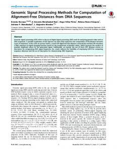
Signal Processing Methods for Genomic Sequence Analysis

Thesis by

Byung-Jun Yoon

In Partial Fulfillment of the Requirements for the Degree of Doctor of Philosophy

California Institute of Technology Pasadena, California

2007 (Defended November 22, 2006)

ii

c 2007

Byung-Jun Yoon All Rights Reserved

iii

Acknowledgments First of all, I would like to express my deepest gratitude to my advisor, Professor P. P. Vaidyanathan, for his excellent guidance and support throughout my graduate studies. In fact, he was the best advisor, mentor, teacher, and researcher, I could ever think of. From my very first day at Caltech, he was always there for me whenever I needed his guidance. He taught me so many important things that are fundamental to a good researcher, for example, how to think creatively, how to develop ideas, how to write good papers, how to be a good presenter, and most importantly, how to stand alone as an independent researcher. It has been my greatest pleasure to learn from P. P., who was the perfect role model. I also would like to thank the members of my defense and candidacy committees: Professor Yaser S. Abu-Mostafa, Professor Babak Hassibi, Professor Christina D. Smolke, Professor Tracey Ho, Professor John Doyle, Professor Changhuei Yang, and Professor Morteza Gharib. I also would like to thank the Microsoft Research, the Korea Foundation for Advanced Studies (KFAS), the National Science Foundation (NSF), and the Office of Naval Research (ONR) for their generous financial support during my graduate studies at Caltech. One of the greatest things at Caltech was the opportunity to work with some of the brightest people in the world! I truly enjoyed working with my labmates in the Digital Signal Processing (DSP) lab, and my warmest appreciation goes to them: Dr. Bojan Vrcelj, Dr. Andre Tkacenko, Sriram Murali, Borching Su, Michael Larsen, Chun-Yang Chen, and Ching-Chih Weng. Thanks to these wonderful guys, working in the DSP lab was a sheer pleasure. I will deeply miss our discussions and conversations as well as the many conference trips that we made together. I also would like to thank Andrea Boyle, our wonderful secretary, for her kind assistance and professional support. During my Ph.D., I had the wonderful opportunity to work at the Microsoft Research (MSR) in Redmond as an intern. I spent three summers at MSR, where I worked with Dr. Henrique (Rico)

iv Malvar during the first two internships and with Dr. Ivan Tashev during the third one. Rico was an extremely good mentor, who showed me what it means to maintain a perfect balance between theoretical research and practical applications. Although he was really busy with his work (well, you may not believe how many meetings he has as a director of MSR), he always found time for discussions and informal chats. I met Ivan during my third internship, where we worked on a project to develop a new adaptive microphone array processing algorithm. Ivan was a passionate mentor and he was very supportive and helpful throughout my internship. In fact, he taught me from A to Z about microphone arrays, although he himself was occupied with so many other things. During the project, I had a chance to build a linear microphone array by myself (it involved designing the array, cutting the plastic board using a laser cutter, soldering the wires, etc.), which was great fun! I am truly grateful to my MSR mentors, Rico and Ivan, who gave me these invaluable experiences that I will never forget. I also would like to express my appreciation to my spiritual mentors, Pastor Chul-Min Kim and Pastor Byungjoo Song. I personally got to know Pastor Kim when I was a college student. At that time, I was still young and immature, and I was not so much interested in spiritual things. However, great passion is contagious, and my life started to change due to his unceasing passion for God and his constant love, care, and prayer for me. If Pastor Kim was the one who planted the seed of faith in me, it was Pastor Song who watered it so that it can grow further. Pastor Song was my mentor for the one-on-one discipleship training at the All Nations Church (a.k.a. Onnuri Church, LA). Being a passionate preacher, good theologian and apologist, he taught me many of the important Christian doctrines in a clear and logical manner. Both mentors have had a crucial impact in shaping myself as a Christian, and I hope I can live as I was taught and as I now believe. One of life’s greatest joys is to meet someone who can (and wants to) truly understand you. In this respect, I was greatly blessed to have many friends with whom I could share every aspect of my life. I am especially thankful to my Caltech friends Wonjin Jang and Hyunjoo Lee, for their friendship and support throughout my graduate studies. I can hardly imagine myself studying at Caltech without these awesome friends. My warmest thanks also goes to Chul-Gi Min and JunSang Lee, my best friends in Korea, whom I have known since my (junior) high-school days. Also, I would like to thank my parents, Choong-Yeol Yoon and Hyo-Kyung Yoo, for their unconditional love and unceasing support throughout my entire life. Their continuous encouragement and prayer have been the very source of power that sustained me during this tumultuous time of

v my life, and I am really indebted to them for their sacrificial love. I am also grateful to my sister, Young-Ran Yoon, for being the best sister I could ever dream of! I also would like to thank my relatives for their encouragements and kind support. Especially, I would like to thank my uncle and aunt, Kang-Yeol Yoon and Nam-Hee Shin, and also aunt Hyo-Im Yoo for their amazing love! Last, but by no means least, I would like to thank God, who has been always so faithful to me. As the apostle Paul has confessed, I am what I am by the amazing grace of God. Even though I did not deserve it, He never stopped loving me, and He has been (and He always will be) leading my life according to His perfect plan that is far beyond my imagination! I pray that I may glorify Him through everything I do, and enjoy Him – and only Him – throughout my entire life. Soli Deo Gloria! To Him be the glory forever and ever. Amen.

vi

Abstract Signal processing is the art of representing, transforming, analyzing, and manipulating signals. It deals with a wide range of signals, from speech and audio signals to images and video signals, and many others. Signal processing techniques have been found very useful in diverse applications. Traditional applications include signal enhancement, denoising, speech recognition, audio and image compression, radar signal processing, and digital communications, just to name a few. In recent years, signal processing techniques have been also applied to the analysis of biological data with considerable success. For example, they have been used for predicting protein-coding genes, analyzing ECG signals and MRI data, enhancing and normalizing DNA microarray images, modeling gene regulatory networks, and so forth. In this thesis, we consider the application of signal processing methods to the analysis of biological sequences, especially, DNA and RNA molecules. We demonstrate how conventional signal processing techniques–such as digital filters and filter banks–can contribute to this end, and also show how we can extend the traditional models–such as the hidden Markov models (HMMs)–to better serve this purpose. The first part of the thesis focuses on signal processing methods that can be utilized for analyzing RNA sequences. The primary purposes of this part are to develop a statistical model that is suitable for representing RNA sequence profiles and to propose an effective framework that can be used for finding new homologues (i.e., similar RNAs that are biologically related) of known RNAs. Many functional RNAs have secondary structures that are well conserved among different species. The RNA secondary structure gives rise to long-range correlations between distant bases, which cannot be represented using traditional HMMs. In order to overcome this problem, we propose a new statistical model called the context-sensitive HMM (csHMM). The csHMM is an extension of the traditional HMM, where certain states have variable emission and transition probabilities that depend on the context. The context-sensitive property increases the descriptive

vii power of the model significantly, making csHMMs capable of representing long-range correlations between distant symbols. Based on the proposed model, we present efficient algorithms that can be used for finding the optimal state sequence and computing the probability of an observed symbol string. We also present a training algorithm that can be used for optimizing the parameters of a csHMM. We give several examples that illustrate how csHMMs can be used for modeling various RNA secondary structures and recognizing them. Based on the concept of csHMM, we introduce profile-csHMMs, which are specifically constructed csHMMs that have linear repetitive structures (i.e., state-transition diagrams). ProfilecsHMMs are especially useful for building probabilistic representations of RNA sequence families, including pseudoknots. We also propose a dynamic programming algorithm called the sequential component adjoining (SCA) algorithm that can systematically find the optimal state sequence of an observed symbol string based on a profile-csHMM. In order to demonstrate the effectiveness of profile-csHMMs, we build a structural alignment tool for RNA sequences and show that the profile-csHMM approach can yield highly accurate predictions at a relatively low computational cost. At the end, we describe how the profile-csHMM can be used for finding homologous RNAs, and we propose a practical scheme for making the search significantly faster without affecting the prediction accuracy. In the second part of the thesis, we focus on the application of digital filters and filter banks in DNA sequence analysis. Firstly, we demonstrate how we can use digital filters for predicting protein-coding genes. Many coding regions in DNA molecules are known to display a period-3 behavior, which can be effectively detected using digital filters. Efficient schemes are proposed that can be used for designing such filters. Experimental results will show that the digital filtering approach can clearly identify the coding regions at a very low computational cost. Secondly, we propose a method based on a bank of IIR lowpass filters that can be used for predicting CpG islands, which are specific regions in DNA molecules that are abundant in the dinucleotide CpG. This filter bank is used to process the sequence of log-likelihood ratios obtained from two Markov chains, where the respective Markov chains model the base transition probabilities inside and outside the CpG islands. The locations of the CpG islands are predicted by analyzing the output signals of the filter bank. It will be shown that the filter bank approach can yield reliable prediction results without sacrificing the resolution of the predicted start/end positions of the CpG islands.

viii

Contents Acknowledgments

iii

Abstract

vi

1

2

Introduction

1

1.1

Discrete Fourier transform (DFT) . . . . . . . . . . . . . . . . . . . . . . . . . . . . . .

2

1.2

Markov chain . . . . . . . . . . . . . . . . . . . . . . . . . . . . . . . . . . . . . . . . .

5

1.3

Hidden Markov model (HMM) . . . . . . . . . . . . . . . . . . . . . . . . . . . . . . .

6

1.4

Review of some fundamentals in genomics . . . . . . . . . . . . . . . . . . . . . . . .

10

1.4.1

DNA and RNA . . . . . . . . . . . . . . . . . . . . . . . . . . . . . . . . . . . .

11

1.4.2

Protein synthesis . . . . . . . . . . . . . . . . . . . . . . . . . . . . . . . . . . .

13

1.4.2.1

Transcription . . . . . . . . . . . . . . . . . . . . . . . . . . . . . . . .

14

1.4.2.2

Translation . . . . . . . . . . . . . . . . . . . . . . . . . . . . . . . . .

16

1.5

RNA secondary structure . . . . . . . . . . . . . . . . . . . . . . . . . . . . . . . . . .

17

1.6

Outline of the thesis . . . . . . . . . . . . . . . . . . . . . . . . . . . . . . . . . . . . . .

18

1.6.1

Context-sensitive hidden Markov models (Chapter 2) . . . . . . . . . . . . . .

18

1.6.2

RNA sequence analysis using context-sensitive HMMs (Chapter 3) . . . . . .

19

1.6.3

Profile context-sensitive hidden Markov models (Chapter 4) . . . . . . . . . .

20

1.6.4

Predicting protein-coding genes using digital filters (Chapter 5) . . . . . . . .

21

1.6.5

Identification of CpG islands using filter banks (Chapter 6) . . . . . . . . . . .

22

Context-Sensitive Hidden Markov Models

23

2.1

Outline . . . . . . . . . . . . . . . . . . . . . . . . . . . . . . . . . . . . . . . . . . . . .

24

2.2

HMMs and transformational grammars . . . . . . . . . . . . . . . . . . . . . . . . . .

25

2.2.1

26

Transformational grammars . . . . . . . . . . . . . . . . . . . . . . . . . . . . .

ix 2.2.2

Palindrome language . . . . . . . . . . . . . . . . . . . . . . . . . . . . . . . . .

28

Context-sensitive hidden Markov models . . . . . . . . . . . . . . . . . . . . . . . . .

29

2.3.1

Basic elements of a csHMM . . . . . . . . . . . . . . . . . . . . . . . . . . . . .

29

2.3.1.1

Hidden states . . . . . . . . . . . . . . . . . . . . . . . . . . . . . . . .

29

2.3.1.2

Observation symbols . . . . . . . . . . . . . . . . . . . . . . . . . . .

31

2.3.1.3

Transition probabilities . . . . . . . . . . . . . . . . . . . . . . . . . .

31

2.3.1.4

Emission probabilities . . . . . . . . . . . . . . . . . . . . . . . . . . .

33

Constructing a csHMM . . . . . . . . . . . . . . . . . . . . . . . . . . . . . . .

33

Finding the most probable path . . . . . . . . . . . . . . . . . . . . . . . . . . . . . . .

34

2.4.1

Alignment of csHMM . . . . . . . . . . . . . . . . . . . . . . . . . . . . . . . .

36

2.4.2

Computing the log-probability of the optimal path . . . . . . . . . . . . . . .

38

2.4.3

Trace-back . . . . . . . . . . . . . . . . . . . . . . . . . . . . . . . . . . . . . . .

44

2.4.4

Computational complexity . . . . . . . . . . . . . . . . . . . . . . . . . . . . .

44

Computing the probability of an observed sequence . . . . . . . . . . . . . . . . . . .

45

2.5.1

Scoring of csHMM . . . . . . . . . . . . . . . . . . . . . . . . . . . . . . . . . .

46

2.5.2

The outside algorithm . . . . . . . . . . . . . . . . . . . . . . . . . . . . . . . .

48

2.6

Estimating the model parameters . . . . . . . . . . . . . . . . . . . . . . . . . . . . . .

52

2.7

Experimental results . . . . . . . . . . . . . . . . . . . . . . . . . . . . . . . . . . . . .

55

2.8

Discussions . . . . . . . . . . . . . . . . . . . . . . . . . . . . . . . . . . . . . . . . . .

58

2.8.1

Emission of multiple symbols . . . . . . . . . . . . . . . . . . . . . . . . . . . .

58

2.8.2

Modeling crossing correlations . . . . . . . . . . . . . . . . . . . . . . . . . . .

59

2.8.3

Comparison with other variants of HMM . . . . . . . . . . . . . . . . . . . . .

61

2.8.4

Comparison with other stochastic grammars . . . . . . . . . . . . . . . . . . .

62

Conclusion . . . . . . . . . . . . . . . . . . . . . . . . . . . . . . . . . . . . . . . . . . .

63

2.3

2.3.2 2.4

2.5

2.9 3

RNA Sequence Analysis Using Context-Sensitive HMMs

64

3.1

Outline . . . . . . . . . . . . . . . . . . . . . . . . . . . . . . . . . . . . . . . . . . . . .

66

3.2

RNA secondary structure . . . . . . . . . . . . . . . . . . . . . . . . . . . . . . . . . .

66

3.3

Searching for homologous RNAs . . . . . . . . . . . . . . . . . . . . . . . . . . . . . .

68

3.3.1

Sequence-based homology search . . . . . . . . . . . . . . . . . . . . . . . . .

69

3.3.2

Statistical model for RNA sequences . . . . . . . . . . . . . . . . . . . . . . . .

70

Database search using csHMMs . . . . . . . . . . . . . . . . . . . . . . . . . . . . . . .

72

3.4

x 3.4.1

Modeling RNA secondary structures . . . . . . . . . . . . . . . . . . . . . . .

72

3.4.2

Database search algorithm . . . . . . . . . . . . . . . . . . . . . . . . . . . . . .

75

3.4.3

Predicting iron response elements . . . . . . . . . . . . . . . . . . . . . . . . .

80

Identification of RNAs with alternative folding . . . . . . . . . . . . . . . . . . . . . .

83

3.5.1

Modeling alternative structures . . . . . . . . . . . . . . . . . . . . . . . . . . .

83

3.5.2

Experimental results . . . . . . . . . . . . . . . . . . . . . . . . . . . . . . . . .

85

3.6

Beyond homology search: Identifying novel ncRNAs . . . . . . . . . . . . . . . . . .

88

3.7

Conclusion . . . . . . . . . . . . . . . . . . . . . . . . . . . . . . . . . . . . . . . . . . .

89

3.5

4

Profile Context-Sensitive Hidden Markov Models

90

4.1

Outline . . . . . . . . . . . . . . . . . . . . . . . . . . . . . . . . . . . . . . . . . . . . .

91

4.2

Profile context-sensitve HMM . . . . . . . . . . . . . . . . . . . . . . . . . . . . . . . .

92

4.2.1

Model construction . . . . . . . . . . . . . . . . . . . . . . . . . . . . . . . . . .

93

4.2.1.1

Constructing an ungapped model . . . . . . . . . . . . . . . . . . . .

93

4.2.1.2

Representing insertions and deletions . . . . . . . . . . . . . . . . .

94

4.2.1.3

Constructing a profile-csHMM from an RNA sequence alignment .

95

Descriptive power . . . . . . . . . . . . . . . . . . . . . . . . . . . . . . . . . .

95

Optimal alignment of profile-csHMM . . . . . . . . . . . . . . . . . . . . . . . . . . .

96

4.3.1

Initialization . . . . . . . . . . . . . . . . . . . . . . . . . . . . . . . . . . . . . .

99

4.3.2

Adjoining subsequences . . . . . . . . . . . . . . . . . . . . . . . . . . . . . . . 100

4.3.3

Adjoining order . . . . . . . . . . . . . . . . . . . . . . . . . . . . . . . . . . . . 102

4.3.4

Termination . . . . . . . . . . . . . . . . . . . . . . . . . . . . . . . . . . . . . . 104

4.3.5

Trace-back . . . . . . . . . . . . . . . . . . . . . . . . . . . . . . . . . . . . . . . 104

4.3.6

Computational complexity . . . . . . . . . . . . . . . . . . . . . . . . . . . . . 105

4.2.2 4.3

4.4

4.5

Structural alignment of RNA pseudoknots . . . . . . . . . . . . . . . . . . . . . . . . 105 4.4.1

Building an alignment tool using the profile-csHMM . . . . . . . . . . . . . . 106

4.4.2

Restricting the search region . . . . . . . . . . . . . . . . . . . . . . . . . . . . 107

4.4.3

Examples of structural alignments . . . . . . . . . . . . . . . . . . . . . . . . . 110

4.4.4

Experimental results . . . . . . . . . . . . . . . . . . . . . . . . . . . . . . . . . 110

Fast search using prescreening filters . . . . . . . . . . . . . . . . . . . . . . . . . . . . 113 4.5.1

Searching for similar sequences . . . . . . . . . . . . . . . . . . . . . . . . . . . 113

4.5.2

Constructing the prescreening filter . . . . . . . . . . . . . . . . . . . . . . . . 115

xi

4.6 5

No degradation in the prediction accuracy . . . . . . . . . . . . . . . . . . . . 116

4.5.4


Conclusion . . . . . . . . . . . . . . . . . . . . . . . . . . . . . . . . . . . . . . . . . . . 118

Predicting Protein-Coding Genes Using Digital Filters

120

5.1

Outline . . . . . . . . . . . . . . . . . . . . . . . . . . . . . . . . . . . . . . . . . . . . . 121

5.2

Period-3 patterns in protein-coding regions . . . . . . . . . . . . . . . . . . . . . . . . 122

5.3

Finding genes from the DNA spectrum . . . . . . . . . . . . . . . . . . . . . . . . . . 122

5.4

5.5

5.6 6

4.5.3

5.3.1

Indicator Sequence . . . . . . . . . . . . . . . . . . . . . . . . . . . . . . . . . . 122

5.3.2

Using DFT for detecting the period-3 patterns . . . . . . . . . . . . . . . . . . 123

5.3.3

Relation to digital filtering . . . . . . . . . . . . . . . . . . . . . . . . . . . . . . 124

IIR antinotch filters . . . . . . . . . . . . . . . . . . . . . . . . . . . . . . . . . . . . . . 126 5.4.1

Designing antinotch filters . . . . . . . . . . . . . . . . . . . . . . . . . . . . . . 126

5.4.2

Implementation of the antinotch filter using a lattice structure . . . . . . . . . 129

5.4.3


Multistage filters . . . . . . . . . . . . . . . . . . . . . . . . . . . . . . . . . . . . . . . 130 5.5.1

Designing a multistage filter . . . . . . . . . . . . . . . . . . . . . . . . . . . . 132

5.5.2

Low complexity implementation . . . . . . . . . . . . . . . . . . . . . . . . . . 133

5.5.3


Conclusion . . . . . . . . . . . . . . . . . . . . . . . . . . . . . . . . . . . . . . . . . . . 135

Identification of CpG Islands Using Filter Banks

137

6.1

Outline . . . . . . . . . . . . . . . . . . . . . . . . . . . . . . . . . . . . . . . . . . . . . 138

6.2

Identification of CpG islands . . . . . . . . . . . . . . . . . . . . . . . . . . . . . . . . 138

6.3

6.2.1

Markov chains . . . . . . . . . . . . . . . . . . . . . . . . . . . . . . . . . . . . 138

6.2.2


Identifying CpG islands using a bank of IIR lowpass filters . . . . . . . . . . . . . . . 142 6.3.1

Filtering the log-likelihood ratios using a filter bank . . . . . . . . . . . . . . . 142

6.3.2


6.3.3

Predicting the transition points between different regions . . . . . . . . . . . 145 6.3.3.1

Rectangular window . . . . . . . . . . . . . . . . . . . . . . . . . . . 145

6.3.3.2

Exponentially decaying window . . . . . . . . . . . . . . . . . . . . . 147

xii 6.4 7

Conclusion . . . . . . . . . . . . . . . . . . . . . . . . . . . . . . . . . . . . . . . . . . . 148

Conclusion

151

A Example of a CFG That Is Not Representable by a csHMM

154

B Algorithms for Sequences with Single Nested Correlations

156

B.1 Simplified alignment algorithm . . . . . . . . . . . . . . . . . . . . . . . . . . . . . . . 156 B.1.1

Computing the log-probability of the optimal path . . . . . . . . . . . . . . . 157

B.1.2

Trace-back . . . . . . . . . . . . . . . . . . . . . . . . . . . . . . . . . . . . . . . 159

B.2 Simplified scoring algorithm . . . . . . . . . . . . . . . . . . . . . . . . . . . . . . . . . 160 C Acronyms

163

Bibliography

165

xiii

List of Figures 1.1

DFTs of periodic signals. (Top) Magnitude plot of the DFT of a signal with a period T = 3. (Bottom) Magnitude plot of the DFT of a signal with a period T = 351/117.5. .

1.2

The DFT of a periodic signal with a period T = 3 buried in Gaussian noise. We can observe a clear peak at k = N/3. . . . . . . . . . . . . . . . . . . . . . . . . . . . . . . .

1.3

6

Illustration of the doubly embedded stochastic process in HMMs. The stochastic process consists of an observable symbol sequence and a hidden state sequence. . . . . .

1.5

4

Example of a state transition diagram that represents a Markov chain with two distinct states S1 and S2 . . . . . . . . . . . . . . . . . . . . . . . . . . . . . . . . . . . . . . . . . .

1.4

3

8

Example of a state transition diagram that represents a hidden Markov model with three states S = {S1 , S2 , S3 } and two distinct observation symbols A = {a, b}. The initial state distribution and the state transition probabilities are shown along the edges and the emission probabilities are shown in the boxes. . . . . . . . . . . . . . . . . . .

8

1.6

Illustration of a nucleotide and a DNA strand. . . . . . . . . . . . . . . . . . . . . . . .

12

1.7

Illustration of a DNA double helix. . . . . . . . . . . . . . . . . . . . . . . . . . . . . . .

12

1.8

Example of a DNA double helix that has been straightened out for simplicity. . . . . .

13

1.9

The central dogma of molecular biology states that the genetic information flows from DNA to RNA to protein. . . . . . . . . . . . . . . . . . . . . . . . . . . . . . . . . . . . .

14

1.10

Illustration of a typical protein synthesis process. . . . . . . . . . . . . . . . . . . . . .

15

1.11

The genetic code. . . . . . . . . . . . . . . . . . . . . . . . . . . . . . . . . . . . . . . . .

16

1.12

Two examples of RNAs with secondary structures. The primary sequence of each RNA is shown along with its structure after folding. The dashed lines indicate interactions between bases. (a) RNA with two stem-loops. (b) RNA with a pseudoknot. . .

2.1

17

The Chomsky hierarchy of transformational grammars nested according to the restrictions on the allowed production rules. . . . . . . . . . . . . . . . . . . . . . . . . . . . .

27

xiv 2.2

Examples of sequences that are included in the palindrome language. The lines indicate the pairwise correlations between distant symbols. . . . . . . . . . . . . . . . . . .

28

2.3

The states Pn and Cn associated with a stack Zn . . . . . . . . . . . . . . . . . . . . . . .

30

2.4

An example of a context-sensitive HMM that generates only palindromes. . . . . . . .

33

2.5

An example of a simple context-sensitive HMM. . . . . . . . . . . . . . . . . . . . . . .

35

2.6

Examples of interactions in a symbol string. The dotted lines indicate the pairwise dependencies between symbols. (a), (b), (c) Nested interactions. (d) Crossing interactions. 37

2.7

Examples of state sequences (a) that are considered in computing γ(i, j, v, w) and (b) those that are not considered. . . . . . . . . . . . . . . . . . . . . . . . . . . . . . . . . .

38

2.8

Illustration of the iteration step of the algorithm. . . . . . . . . . . . . . . . . . . . . . .

42

2.9

Illustration of the iteration step of the algorithm for the case when si = Pn and sj = Cn . 43

2.10

Examples of state sequences (a) that are considered in computing β(i, j, v, w) and (b) those that are not considered. . . . . . . . . . . . . . . . . . . . . . . . . . . . . . . . . .

2.11

Illustration of the iteration step of the outside algorithm. (a) Case (ii). (b) Case (iii). (c) Case (iv). . . . . . . . . . . . . . . . . . . . . . . . . . . . . . . . . . . . . . . . . . . . . .

2.12

48

51

Illustration of the iteration step of the outside algorithm. (a) Case (v). (b) Case (vi). (c) Case (viii). . . . . . . . . . . . . . . . . . . . . . . . . . . . . . . . . . . . . . . . . . . . .

52

2.13

An example of a context-sensitive HMM. . . . . . . . . . . . . . . . . . . . . . . . . . .

55

2.14

The arithmetic mean (top) and the geometric mean (bottom) after each iteration. . . .

58

2.15

An example sequence that can be generated by the modified model of Figure 2.4. . . .

59

2.16

(a) A csHMM that results in crossing interactions. (b) An example of a generated symbol sequence. The lines indicate the correlations between symbols. . . . . . . . . .

2.17

(a) A csHMM that represents a copy language. (b) An example of a generated symbol sequence.

2.18

60

. . . . . . . . . . . . . . . . . . . . . . . . . . . . . . . . . . . . . . . . . . . .

60

An illustration of the basic concept of the algorithm that can be used when there exist crossing interactions. The dotted lines show examples of correlations that can be taken

2.19

into consideration based on this setting. . . . . . . . . . . . . . . . . . . . . . . . . . . .

61

The csHMM in the Chomsky hierarchy. . . . . . . . . . . . . . . . . . . . . . . . . . . .

63

xv 3.1

Two common mechanisms of riboswitches in bacteria. (a) Translation control. In the presence of the effector metabolite, the riboswitch changes its structure and sequesters the ribosome-binding site (RBS). This inhibits the translation initiation, thereby downregulating the gene. (b) Transcription control. Upon binding the metabolite, the riboswitch forms a terminator stem, which prevents the generation of the full-size mRNA. 67

3.2

An example of a profile-HMM. It repetitively uses a set of match, insert, and delete states to model each position in a multiple sequence alignment. . . . . . . . . . . . . .

3.3

69

Ungapped alignment between two RNA sequences. (a) An RNA with a stem-loop structure is used as the query sequence. (b) A structurally homologous RNA that has also a stem-loop structure. (c) A structurally nonhomologous RNA that does not fold to a stem-loop structure. . . . . . . . . . . . . . . . . . . . . . . . . . . . . . . . . . . . .

3.4

Compensatory mutations give rise to strong pairwise correlations in the primary sequence of an RNA. . . . . . . . . . . . . . . . . . . . . . . . . . . . . . . . . . . . . . . .

3.5

70

71

(a) A typical stem-loop. The nodes represent the bases in the RNA, and the dotted lines indicate the interactions between bases that form complementary base pairs. (b) An example of a csHMM that generates a sequence with a stem-loop structure. (c) A csHMM that models a stem-loop with bulges. . . . . . . . . . . . . . . . . . . . . . . .

3.6

(a) A typical structure of an iron response element. (b) An example of a csHMM that generates sequences with the given secondary structure. . . . . . . . . . . . . . . . . .

3.7

74

(a) A typical tRNA cloverleaf structure. (b) An example of a csHMM that can generate sequences with the cloverleaf structure. . . . . . . . . . . . . . . . . . . . . . . . . . . .

3.8

74

75

Two different update schemes. (a) When using the variable γ(i, d, v, w). (b) When using the variable γ(j, d, v, w). . . . . . . . . . . . . . . . . . . . . . . . . . . . . . . . . .

77

3.9

Illustration of step (v). . . . . . . . . . . . . . . . . . . . . . . . . . . . . . . . . . . . . .

78

3.10

Illustration of step (vi). . . . . . . . . . . . . . . . . . . . . . . . . . . . . . . . . . . . . .

79

3.11

Illustration of step (vii). . . . . . . . . . . . . . . . . . . . . . . . . . . . . . . . . . . . .

80

3.12

The consensus secondary structures of the iron response elements (IREs). . . . . . . .

81

3.13

A csHMM that represents the IREs. . . . . . . . . . . . . . . . . . . . . . . . . . . . . .

82

3.14

An antiswitch regulator. (a) Secondary structure of the antiswitch in the absence of ligand. (b) The structure changes upon binding the ligand. (c) In the presence of ligand, the antiswitch can bind to the target mRNA, suppressing its expression. . . . .

84

xvi 3.15

Base correlations in the primary sequence of an antiswitch. (a) Overall correlations. (b) Correlations due to structure 1 (in the absence of ligand). (c) Correlations due to structure 2 (in the presence of ligand). . . . . . . . . . . . . . . . . . . . . . . . . . . . .

85

3.16

(a) The csHMM that represents structure 1. (b) The csHMM that represents structure 2. 86

3.17

Plot of (S1 (x), S2 (x)). . . . . . . . . . . . . . . . . . . . . . . . . . . . . . . . . . . . . . .

87

4.1

Relation between profile-csHMMs and other statistical models. . . . . . . . . . . . . .

92

4.2

Constructing a profile-csHMM from an RNA multiple sequence alignment. (a) An alignment of five RNA sequences. The consensus RNA secondary structure has two base pairs. (b) Ungapped profile-csHMM that represents the consensus RNA sequence. (c) The final profile-csHMM that allows additional insertions and deletions at any location. . . . . . . . . . . . . . . . . . . . . . . . . . . . . . . . . . . . . . . . . . . .

4.3

Various types of RNA secondary structures. (a) RNA with 2-crossing property. (b) RNA with 3-crossing property. (c) RNA with 4-crossing property. . . . . . . . . . . . .

4.4

94

96

(a) An RNA sequence with no structural annotation. (b) Optimal state sequence of the observed RNA sequence in the given profile-csHMM. (c) Structural alignment obtained from the optimal state sequence. . . . . . . . . . . . . . . . . . . . . . . . . . . .

4.5

97

The adjoining order of the profile-csHMM shown in Figure 4.2. This illustrates how we can adjoin the base and the base pairs in the consensus RNA sequence to obtain the entire sequence. . . . . . . . . . . . . . . . . . . . . . . . . . . . . . . . . . . . . . . . 103

4.6

Matching bases in an RNA sequence alignment. (a) The maximum distance between the matching bases is two. (b) The maximum distance between the matching bases is seven. . . . . . . . . . . . . . . . . . . . . . . . . . . . . . . . . . . . . . . . . . . . . . . . 108

4.7

Limiting the search region for finding the matching bases can significantly reduce the overall complexity of the structural alignment. . . . . . . . . . . . . . . . . . . . . . . . 108

4.8

Structural alignments of RNAs with various secondary structures. . . . . . . . . . . . 109

4.9

Structural alignment of two RNAs in the F LAVI

PK 3

family. The secondary structure

of the target RNA has been predicted from the given alignment. Incorrect predictions (one false negative and two false positives) have been underlined. . . . . . . . . . . . 112 4.10

Illustration of the proposed algorithm. . . . . . . . . . . . . . . . . . . . . . . . . . . . . 115

5.1

The magnitude response of the sliding window w(n). . . . . . . . . . . . . . . . . . . . 125

xvii 5.2

The indicator sequence xB (n) is passed through the bandpass filter H(z). The output yB (n) will be large in the coding regions due to the period-3 component. . . . . . . . . 126

5.3

Poles and zeros of the notch filter G(z) and the allpass filter A(z). . . . . . . . . . . . . 127

5.4

Magnitude response of the notch filter G(z) for two values of R. . . . . . . . . . . . . . 128

5.5

Magnitude response of the antinotch filter H(z) for two values of R. . . . . . . . . . . 128

5.6

Implementation of the antinotch filter H(z) = V (z)/X(z) using a lattice structure. . . 129

5.7

Exon prediction results for the gene F56F11.4 in the C. elegans chromosome III. (Top) Plot of S[N/3] computed using the DFT. (Bottom) Plot of Y (n) that is computed using the antinotch filter. . . . . . . . . . . . . . . . . . . . . . . . . . . . . . . . . . . . . . . . 131

5.8

Designing a bandpass filter based on multistage filtering. (a) Magnitude response of the prototype narrowband lowpass filter H1 (z). (b) Magnitude response of H1 (z 3 ). (c) Magnitude response of H2 (z) that can be used to eliminate the undesirable passband of H1 (z 3 ) at ω = 0. . . . . . . . . . . . . . . . . . . . . . . . . . . . . . . . . . . . . . . . 132

5.9

Multistage filtering. . . . . . . . . . . . . . . . . . . . . . . . . . . . . . . . . . . . . . . . 133

5.10

Magnitude response of the filters used in the multistage design method. (a) Lowpass elliptic filter H1 (z). (b) The response of the filter H1 (z 3 ). (c) FIR lowpass filter H2 (z). (d) The magnitude response of the cascaded filter H(z) = H1 (z 3 )H2 (z). . . . . . . . . 134

5.11

Exon prediction results for the gene F56F11.4 in the C. elegans chromosome III. (Top) Plot of the output S[N/3] of the DFT-based approach. (Middle) Plot of the output of the antinotch filter method. (Bottom) Plot of the output of the multistage filter approach.136

6.1

(Top) CpG island prediction result obtained by the conventional Markov chain method. (Bottom) Magnified plot. We can see that there are many undesirable zero crossings due to the fluctuations of S(n). . . . . . . . . . . . . . . . . . . . . . . . . . . . . . . . . 141

6.2

A bank of M lowpass filters with different bandwidths. . . . . . . . . . . . . . . . . . . 143

6.3

Contour plot of the outputs Sk (n). The red band in the middle clearly indicates the existence of a CpG island. . . . . . . . . . . . . . . . . . . . . . . . . . . . . . . . . . . . 144

6.4

Two level contour plot of the outputs Sk (n). The level curve is located at zero, separating the positive and the negative regions. . . . . . . . . . . . . . . . . . . . . . . . . 144

6.5

A rectangular window of length L located around the transition point. . . . . . . . . . 146

6.6

An exponentially decaying window located around the transition point. . . . . . . . . 148

6.7

The delay k ∗ corresponding to the value αk . . . . . . . . . . . . . . . . . . . . . . . . . 149

xviii 6.8

Actual level curves for S(n) = 0 against the theoretical curve (thick line with diamonds) computed from the transition probabilities. (Top) Region changes from a non-CpG island region to a CpG island. (Bottom) Region changes from a CpG island to a non-CpG island region. . . . . . . . . . . . . . . . . . . . . . . . . . . . . . . . . . . 149

A.1

Constructions which guarantee that the number of “a’s” and the number of “b . . . bc’s” in x1 . . . xL−N are identical. . . . . . . . . . . . . . . . . . . . . . . . . . . . . . . . . . . 155

B.1

Examples of symbol sequences with different correlation structures. Sequences with single-nested correlations are shown in (a) and (b), and sequences with multiplenested correlations are shown in (c) and (d). . . . . . . . . . . . . . . . . . . . . . . . . 157

B.2

Illustration of the iteration step of the simplified scoring algorithm. . . . . . . . . . . . 162

xix

List of Tables 2.1

The Chomsky hierarchy of transformational grammars. . . . . . . . . . . . . . . . . . .

26

2.2

Computational complexity of the csHMM alignment algorithm. . . . . . . . . . . . . .

45

2.3

Emission probabilities e(x|v). . . . . . . . . . . . . . . . . . . . . . . . . . . . . . . . . .

56

2.4

Estimated emission probabilities e(x|v) after 10 iterations. . . . . . . . . . . . . . . . .

57

3.1

The database search result for finding IREs. . . . . . . . . . . . . . . . . . . . . . . . . .

82

4.1

Prediction results of the proposed method for several RNA families with pseudoknot structures. The prediction results of PSTAGs are also shown for comparison. The prediction results of PSTAGs are obtained from [66]. . . . . . . . . . . . . . . . . . . . . 111

4.2

CPU time for aligning two sequences in each RNA family. The experiments have been performed on a PowerMac G5 Quad 2.5 GHz with 4 GB memory. . . . . . . . . . . . . 111

4.3

Prediction results of the proposed method using randomly mutated RNA sequences.

112

6.1

Transition probabilities inside the CpG island region. . . . . . . . . . . . . . . . . . . . 140

6.2

Transition probabilities in the non-CpG island region. . . . . . . . . . . . . . . . . . . . 140

1

Chapter 1

Introduction Signal processing is the art of representing, transforming, analyzing, and manipulating signals. It deals with a large variety of signals, including speech and audio signals, images and video signals, and even biological signals such as DNA sequences, ECG signals, MRI signals, and so forth. Signal processing techniques have been found useful in truly diverse applications, such as signal enhancement [33], denoising [14, 101], speech recognition [82], audio [73] and image compression [100, 118], radar signal processing [84], and digital communications [42, 43], just to name a few. More recently, signal processing techniques have been also applied to the analysis of biological data with considerable success. For example, they have been utilized for the prediction of proteincoding genes [3, 106], characterization of ECG signals [63, 94], representation of gene regulatory networks [99], analysis of DNA microarray images [13, 115], and many others. The reader who is interested in the recent advances of signal processing methods in biology is referred to the following tutorial reviews [3, 22, 23, 112, 113, 130]. The primary focus of the thesis lies in the application of signal processing concepts to the analysis of genomic sequence data. Among other things, this thesis presents various signal processing methods–such as digital filters, filter banks, and variants of HMMs (hidden Markov models)–that have been found especially useful in analyzing DNA and RNA sequence data and identifying regions of specific interest–e.g., protein-coding genes, CpG islands, and noncoding RNA (ncRNA) genes–inside these sequences. A more detailed outline of the thesis is presented in Section 1.6 of this Chapter. The main purpose of this introductory Chapter is to equip the readers with some fundamentals in signal processing and genomics that are needed to understand the technical details of the discussions that will follow. We make every attempt to make this Chapter as self-contained as possible, in

2 order to serve this purpose. In Section 1.1 we briefly describe the discrete Fourier transform (DFT) that can be used for isolating the signal component with certain periodicity. The basic concepts of Markov chains and hidden Markov models (HMMs) are reviewed in Section 1.2 and Section 1.3, respectively. In Section 1.4, we review some fundamentals in genomics, and in Section 1.5, we briefly describe the concept of RNA secondary structures. The material presented in this Chapter is only meant to be a quick introduction to signal processing and genomics, and it is by no means a complete and comprehensive coverage of these topics. For a more extensive treatment of these topics, the reader is referred to the references given at the end of each section.

1.1

Discrete Fourier transform (DFT)

Let us consider a finite length signal x(n) whose length is N . We assume that x(n) = 0 outside the range 0 ≤ n ≤ N − 1. The discrete Fourier transform (DFT) of x(n) is defined as

X[k] =

N −1 X

x(n)W kn ,

(1.1)

n=0

where W = e−j2π/N . Sometimes, we may assume that the signal x(n) has length N even when its actual length is smaller. For example, it is possible that x(n) = 0 outside the range 0 ≤ n ≤ L = M − 1, where M ≤ N . For this reason, the transform in (1.1) is sometimes called the N -point DFT, in order to prevent any ambiguity. As the Fourier transform of x(n) is defined as X(ejω ) =

X

x(n)e−jwn ,

(1.2)

n

we can view the DFT X[k] of a signal x(n) as a uniformly sampled version of X(ejω ) at frequencies ωk =

2πk N

for k = 0, 1, . . . , N − 1. Given the DFT coefficients X[k], we can reconstruct the original

signal x(n) as follows x(n) =

N −1 1 X X[k]W −kn . N

(1.3)

k=0

This transform is called the inverse-DFT of X[k]. There exist efficient algorithms for computing the DFT and its inverse (IDFT), which are collectively called the fast Fourier transform (FFT) algorithms [24]. While the direct computation of the (N -point) DFT coefficients requires O(N 2 ) opera-

3

350 300

|X1[k]|

250 200 150 100 50 0

0

50

100

150

200

250

300

350

200

250

300

350

k 350 300

|X2[k]|

250 200 150 100 50 0

0

50

100

150

k

Figure 1.1: DFTs of periodic signals. (Top) Magnitude plot of the DFT of a signal with a period T = 3. (Bottom) Magnitude plot of the DFT of a signal with a period T = 351/117.5.

tions, the FFT algorithm can compute the DFT in only O(N log N ) operations.1 The DFT X[k] of a signal x(n) can effectively analyze the frequency components contained in x(n). For example, the DFT coefficient X[k] shows the strength of the signal component whose frequency is located at (or near) ω = 2πk/N . This corresponds to the period T = N/k in the time domain. Let us consider a finite-length periodic signal x1 (n) defined as follows x1 (n) = ej2πn/3 , 0 ≤ n ≤ N − 1,

(1.4)

where the length of the signal is N = 351. As the period of x1 (n) if 3, its DFT X1 [k] = DFT[x1 (n)] should have a peak at ω = 2π/3. This is demonstrated in Figure 1.1 (Top), where the magnitude of the DFT X1 [k] has only a single peak at k = N/3 = 117. When the frequency of the input signal is not located at one of the frequencies ωk = 1 The

notation O(·) means “on the order of”.

2πk N

(k = 0, 1, . . . , N − 1), its energy will be distributed

4

350

300

|X3[k]|

250

200

150

100

50

0

0

50

100

150

200

250

300

350

k

Figure 1.2: The DFT of a periodic signal with a period T = 3 buried in Gaussian noise. We can observe a clear peak at k = N/3.

over several frequency bins. For example, let us consider another periodic signal x2 (n) defined as x2 (n) = ej2π

(N/3)+0.5 n N

, 0 ≤ n ≤ N − 1,

where N = 351 is the same as before. The magnitude plot of the DFT X2 [k] = DFT[x2 (n)] is shown in Figure 1.1 (Bottom). We can see that the there are many non-zero DFT coefficients in this case, although the peak is located near k =

N/3+0.5 . N

Finally, let us consider a periodic signal that is buried in noise. We define x3 (n) = x1 (n) + z(n), 0 ≤ n ≤ N − 1 where x1 (n) is a periodic signal with period T = 3 as defined in (1.4) and z(n) is white Gaussian noise with unit variance. The magnitude plot of X3 [k] = DFT[x3 (n)] is shown in Figure 1.2. In Figure 1.2, we can clearly observe the peak at k = N/3 that corresponds to the period T = 3 of the signal x1 (n). In Chapter 5, we will show how this property can be used for identifying protein-coding regions in DNA sequences. Further details of the DFT and its basic properties can be found in [74].

5

1.2

Markov chain

Let us consider a system that can be described by one of a finite number of states S = {S1 , . . . , SM }. At each discrete time index n, the state yn of the system takes one of the values yn ∈ S. The system makes a state-transition at each unit time, which gives rise to a sequence of states y0 → y1 → y2 → . . . → yn .

(1.5)

We say that this discrete-time stochastic process satisfies the Markov property, if the probability distribution of the future state yn+1 depends only on the present state yn and not on the past states yn−k (k ≥ 1). This can be written as P (yn+1 = Sj |yn = Si , yn−1 = Sk , yn−2 = S` , . . .) = P (yn+1 = Sj |yn = Si ).

(1.6)

In this case, the state sequence in (1.5) is called a first-order Markov chain (Markov model). If the transition probability shown in (1.6) is time independent such that P (yn+1 = Sj |yn = Si ) = t(Si , Sj ), for all n, it is called a stationary Markov chain. The transition probabilities t(Si , Sj ) satisfy

M X

t(Si , Sj ) ≥ 0

(1 ≤ i, j ≤ M ),

t(Si , Sj )

(1 ≤ i ≤ M ).

=

1

j=1

As we can see from above, a stationary Markov chain is completely governed by its state transition probabilities t(Si , Sj ), and it can be conveniently represented by a state transition diagram. An example of such a diagram is shown in Figure 1.3. Unless mentioned otherwise, we assume that the Markov chain that is being used is stationary. In many applications, Markov chains are used to model the correlations between observable physical events. Every state represents a distinct event, and the state transition probabilities describe the correlations between these events. Once we have constructed a model that properly describes the system that gives rise to the observable events, this model can be used to evaluate the probability of observing a series of events. For example, let us consider the following problem.

6

t(S1,S2) t(S1,S1)

S1

S2

t(S2,S2)

t(S2,S1) Figure 1.3: Example of a state transition diagram that represents a Markov chain with two distinct states S1 and S2 .

Given that the current state is y0 ∈ S, how can we compute the probability that the next L states will be exactly y1 y2 . . . yL ? Using the Markov property, this probability can be simply computed as

P (y1 y2 . . . yL |y0 )

=

L Y

P (yn |yn−1 )

n=1

=

L Y

t(yn−1 , yn ).

(1.7)

n=1

Consider the case when we have multiple Markov chains, where each model describes the behavior of a system under different conditions. In this case, we can use the observation probability in (1.7) to determine which model describes the observed events best. The Markov chains are utilized in Chapter 6, where they are used to represent the base sequences inside CpG islands and those outside CpG islands. It is demonstrated that they can be effectively used for discriminating CpG islands from the non-CpG island regions. For further details on Markov chains, the reader is referred to [89].

1.3

Hidden Markov model (HMM)

For many real world problems, the assumption that each state in the Markov chain corresponds to an “observable” event may be too restrictive. In such cases, we can use the hidden Markov model (HMM) that is an extension of the simpler Markov model. The HMM is a doubly embedded stochastic process that consists of an invisible process of hidden states and a visible process of observable symbols (or events). The hidden state sequence satisfies the Markov property, which is governed by the state transition probabilities associated with the model. The probability distribution of the observed symbols depend on the underlying states. More formally, this can be written

7 as follows. Let xn ∈ A be the observed symbol at time n, where A = {a1 , . . . , aN } is the set of all observable symbols. We denote the underlying state at time n as yn ∈ S, where S = {S1 , . . . , SM } is the set of distinct states in the hidden Markov model. As the state sequence satisfies the Markov property, we have P (yn+1 = Sj |yn = Si , yn−1 = Sk , . . .)

= P (yn+1 = Sj |yn = Si ) = t(Si , Sj ).

At time n, the emission probability of the observed symbol xn depends on the hidden state yn P (xn = ak |yn = S` ) = e(ak |S` ). Note that t(Si , Sj ) is the stationary state transition probability from state Si to state Sj , and e(ak |S` ) is the stationary symbol emission probability of symbol ak at state S` . The stochastic process of hidden states and the process of observable symbols are illustrated in Figure 1.4. In general, the hidden state sequence (typically called a “path”) cannot be directly inferred from the observed symbol sequence, although some information about the state sequence can be obtained from the observation. An HMM is completely defined by the set of parameters Θ = {T, E, π}, where the matrices T = {tij } and E = {e`k } and the vector π = {πi } are defined as follows.

tij

= t(Si , Sj ),

e`k

= e(ak |S` ),

πi

= P (y1 = Si ),

for 1 ≤ i, j, ` ≤ M and 1 ≤ k ≤ N . T is the transition probability matrix, E is the emission probability matrix, and π is the initial state distribution of the model. Like Markov chains, HMMs can also be conveniently represented by state transition diagrams. Figure 1.5 shows an example of such a diagram. The HMM shown in Figure 1.5 has the following

8

x1

x2 e(x1|y1)

y1

x3 e(x2|y2)

y2 t(y1,y2)

x4 e(x3|y3)

e(x4|y4)

y3 t(y2,y3)

x5

y4 t(y3,y4)

observed symbols e(x5|y5)

… hidden states

y5 t(y4,y5)

Figure 1.4: Illustration of the doubly embedded stochastic process in HMMs. The stochastic process consists of an observable symbol sequence and a hidden state sequence.

START 0.4

0.6

0.7 0.3

S1

S1

S2

0.3

0.2

a:a:0.8 0.8 b: 0.2 b: 0.2

0.5

S2

a:a:0.3 0.3 b: 0.7 b: 0.7

0.9

S3 S3

0.1

a:a:0.5 0.5 b:b:0.5 0.5

Figure 1.5: Example of a state transition diagram that represents a hidden Markov model with three states S = {S1 , S2 , S3 } and two distinct observation symbols A = {a, b}. The initial state distribution and the state transition probabilities are shown along the edges and the emission probabilities are shown in the boxes.

9 set of parameters Θ = {T, E, π}  T

E

π

0.3

0.7

  =  0.2 0.3  0.9 0.0  0.8 0.2   =  0.3 0.7  0.5 0.5 h = 0.6 0.4

0.0



  0.5  ,  0.1    ,  0.0

i

.

As an example, let us consider the following observation sequence x with the underlying state sequence y as shown below x

=

a

a

b

b

a,

y

= S1

S1

S2

S3

S1 .

The probability P (x, y) can be computed as

P (x, y)

= P (y1 = S1 ) × e(a|S1 ) × t(S1 , S1 ) × e(a|S1 ) × t(S1 , S2 ) ×e(b|S2 ) × t(S2 , S3 ) × e(b|S3 ) × t(S3 , S1 ) × e(a|S1 ) =

0.6 × 0.8 × 0.3 × 0.8 × 0.7 × 0.7 × 0.5 × 0.5 × 0.9 × 0.8

=

1.016064 × 10−2 .

There are three important problems that have to be solved in order to apply the HMMs to real world applications. These problems are typically called the alignment problem, the scoring problem, and the training problem. These problems are described in the following. Alignment problem Given an observed symbol sequence x = x1 x2 . . . xL and an HMM defined by the set of parameters Θ, how can we find the optimal state sequence y = y1 y2 . . . yL that maximizes the observation probability P (y|x, Θ)? This is called the “alignment problem” because it tries to find the best alignment between the symbol sequence x and the given HMM. As the number of paths increases exponentially with the length L of the symbol string x, comparing all paths is practically infeasible. However, there exists an efficient dynamic programming algorithm called the Viterbi algorithm, which can find the optimal state sequence in a systematic

10 way [116]. The complexity of the Viterbi algorithm is only O(LM 2 ), which increases linearly with respect to the sequence length L, where M is the number of states. Scoring problem Given an observed symbol sequence x = x1 x2 . . . xL , how can we compute its observation probability based on a given model Θ? As this probability can be used to score different models to choose the one that best describes the observation sequence, it is usually called the “scoring problem.” This problem can be efficiently solved using the forward algorithm [56, 81], which is closely related to the Viterbi algorithm. The complexity of the forward algorithm is also O(LM 2 ). Training problem Finally, we have to address the problem of how to choose the model parameters in an optimal manner, based on a number of training sequences. One popular solution to this problem is an EM (expectation-maximization) algorithm called the Baum-Welch algorithm [6]. This algorithm can iteratively find the parameters that achieve a local maximum of the observation probability of the training sequences. The algorithms that can be used for solving these problems for HMMs are described in considerable detail in [56, 81]. HMMs are well known for their effectiveness in modeling short-term dependencies between adjacent symbols. For this reason, they have been extensively used in various fields, including speech recognition [56, 81] and bioinformatics [28, 59]. In Chapter 2, we extend the traditional HMM so that we can also describe long-range correlations between distant symbols. The extended model, called the context-sensitive HMM (csHMM) has important applications in RNA sequence analysis, as will be demonstrated in Chapter 3 and Chapter 4.

1.4

Review of some fundamentals in genomics

In this section, we briefly review some basics in genomics that are needed to understand the details of the thesis.

11

1.4.1

DNA and RNA

DNA (deoxyribonucleic acid) is a nucleic acid that contains the genetic information for cellular life forms and viruses. They are responsible for propagating the hereditary information in all living organisms. A single strand of DNA consists of many nucleotides that are linked to each other forming a long chain. A nucleotide consists of a base, a sugar, and a phosphate (or a phosphate group). The structure of a nucleotide is illustrated in Figure 1.6. The nucleotides that form a DNA strand can have four different kinds of bases, namely, adenine, cytosine, guanine, and thymine. For convenience, these nucleotides (or the bases) are typically represented by the four letters A, C, G, and T. In general, a single strand of DNA forms a double helix with another single strand of DNA via hydrogen bonding between the bases. An illustration of a DNA double helix is shown in Figure 1.7. The nucleotide A in one strand is linked to T in the other strand (and vice versa), and the nucleotide C in one strand is connected to G in the other strand (and vice versa). As a result, one strand in a DNA double helix completely determines the nucleotide sequence in other strand, hence they are called complementary strands. Figure 1.8 shows an example of a short DNA double helix that has been straightened out for simplicity. As indicated in the figure, the sugar-phosphate forms the backbone of each DNA strand, and the two strands that run towards opposite directions are linked to each other by the chemical bonds formed between the complementary bases. As the nucleotide sequence in one strand determines the nucleotide sequence in the other strand, a double-stranded DNA can be unambiguously represented by either strand. For this reason, a DNA molecule is represented by the nucleotide sequence of the forward strand, which is read from the so-called 5’-end to the 3’-end. For example, let us consider the DNA shown in Figure 1.8: 50 − A − A − T − C − G − G − C − T − A − C − 30

(forward strand)

30 − T − T − A − G − C − C − G − A − T − G − 50

(backward strand) .

This can be simply represented by the forward strand 50 − A − A − T − C − G − G − C − T − A − C − 30 .

Therefore, from a signal processing perspective, we can view a DNA molecule as a symbol se-

12

sugar phosphate

5’

3’

A

A

T

G

C

base nucleotide

DNA strand

Figure 1.6: Illustration of a nucleotide and a DNA strand.

G

C 3’

G

C

T

A

G

C A

T A

T

3.4nm (34A)

G

sugar-phosphate backbone

C

T

A

C

G A

T G

A

C

T

Figure 1.7: Illustration of a DNA double helix.

5’

13 sugar-phosphate backbone

5’

3’

A

A

T

C

G

G

C

T

A

C

T

T

A

G

C

C

G

A

T

G

3’

forward strand

5’

backward strand

bases

Figure 1.8: Example of a DNA double helix that has been straightened out for simplicity. quence, where the symbols are taken from a finite alphabet. The RNA (ribonucleic acid) is another type of nucleic acid that is closely related to the DNA. It also consists of four kinds of bases like the DNA, except that uracil (U) is used instead of thymine (T). Unlike DNA molecules, the RNA is typically a single-stranded molecule.

1.4.2

Protein synthesis

A protein is a complex biomolecule that consists of a long chain of amino acids. The amino acids are linked to each other by strong covalent bonding called peptide bonds, and the amino acid chain is also known as a polypeptide. There are 20 different kinds of amino acids in proteins, where each amino acid has a different side-chain. Therefore, a protein can be conveniently represented as a sequence of amino acids, where each of the 20 distinct amino acids is denoted by a 3-letter code or an 1-letter code. For example, the amino acid alanine is denoted by ‘Ala’ or ‘A,’ and cysteine is denoted by ‘Cys’ or ‘C.’ Proteins are involved in every single biological process in all cells, hence playing a crucial role in all living organisms. The information that is needed for encoding proteins is stored in the DNA. Portions in the DNA that contain the information for producing proteins are called protein-coding genes, or often simply genes.2 Each gene in the DNA is first copied into an RNA molecule (transcription), which is then used to produce proteins (translation). Therefore, it can be said that the genetic information flows from DNA to RNA to protein. This basic principle is typically called the central dogma of molecular biology [1], and it explains how the genetic instructions contained in the DNA are used to synthesize RNAs and proteins. Figure 1.9 illustrates this principle in a simple diagram. The main steps in a typical protein synthesis process are shown in Figure 1.10. Each step in the process is discussed in the following subsections. 2 Note that there exist also ncRNA (noncoding RNA) genes, which are portions of DNA that give rise to functional RNAs that are not translated into proteins.

14

DNA

RNA synthesis (transcription) RNA

Protein synthesis (translation) Protein

Figure 1.9: The central dogma of molecular biology states that the genetic information flows from DNA to RNA to protein. 1.4.2.1

Transcription

The process of copying the content of a gene into an RNA is called transcription. The transcription process is carried out by an enzyme called RNA polymerase, where an enzyme is a protein that catalyzes a specific chemical reaction. Initially, the RNA polymerase binds to a special region in the DNA called the promoter, which is located upstream of a gene and is used to designate the starting point of the transcription process. During transcription, the RNA polymerase uses one strand of the DNA (called the template strand) to copy the content into an RNA molecule. While copying the content from DNA to RNA, a thymine (T) in the original DNA sequence is replaced by a uracil (U) in the RNA that is being synthesized. The resulting transcript of a protein-coding gene is called a pre-mRNA (pre-messenger RNA). Living organisms can be categorized into two types, namely, prokaryotes and eukaryotes. Prokaryotes are simple organisms (mostly unicellular) that do not have a cell nucleus. Bacteria are common examples of prokaryotes. On the other hand, eukaryotes are organisms that have complex cells with membrane-bound nuclei. Most of them are multicellular, and higher organisms such as worms, plants, insects and mammals belong to eukaryotes. Most protein-coding genes in eukaryotes consist of two types of regions called exons and introns (see Figure 1.10).3 The introns are removed from the pre-mRNA and the remaining exons are concatenated to form a mRNA (messenger RNA). This process is called splicing. Sometimes, one pre-mRNA gives rise to multiple mRNAs 3 The

protein-coding genes of prokaryotes do not have introns.

15

Gene A

Gene B

Gene C

DNA

(a) Transcription

(b)

Pre-mRNA 5’ UTR

Exon 1

Intron

Exon 2

Intron

Exon 3

Splicing

(c)

mRNA 1

mRNA 2

mRNA Exon 1

Exon 2

Exon 1

Exon 3

Translation

(d) Protein Protein 1

Protein 2

Figure 1.10: Illustration of a typical protein synthesis process.

3’ UTR

16

UUU : Phenylalanine UUC : Phenylalanine UUA : Leucine UUG : Leucine

UCU : Serine UCC : Serine UCA : Serine UCG : Serine

UAU : Tyrosine UAC : Tyrosine UAA : Stop UAG : Stop

UGU : Cysteine UGC : Cysteine UGA : Stop UGG : Tryptophan

CUU : Leucine CUC : Leucine CUA : Leucine CUG : Leucine

CCU : Proline CCC : Proline CCA : Proline CCG : Proline

CAU : Histidine CAC : Histidine CAA : Glutamine CAG : Glutamine

CGU : Arginine CGC : Arginine CGA : Arginine CGG : Arginine

AUU : Isoleucine AUC : Isoleucine AUA : Isoleucine AUG : Methionine, Start

ACU : Threonine ACC : Threonine ACA : Threonine ACG : Threonine

AAU : Asparagine AAC : Asparagine AAA : Lysine AAG : Lysine

AGU : Serine AGC : Serine AGA : Arginine AGG : Arginine

GUU : Valine GUC : Valine GUA : Valine GUG : Valine

GCU : Alanine GCC : Alanine GCA : Alanine GCG : Alanine

GAU : Aspartic acid GAC : Aspartic acid GAA : Glutamic acid GAG : Glutamic acid

GGU : Glycine GGC : Glycine GGA : Glycine GGG : Glycine

Figure 1.11: The genetic code. by combining different exons. This phenomenon is called alternative splicing, and it is widely observed in eukaryotes. 1.4.2.2

Translation

During the translation process, the mRNA that was transcribed from DNA is decoded by the ribosome and tRNAs (transfer RNA) to generate a polypeptide (or a protein). A polypeptide is a long sequence of amino acids that are interconnected via peptide bonds. The translation of mRNAs into proteins is governed by the genetic code that maps each of the 64 codons (triplets of nucleotides) into one of the 20 different amino acids. Figure 1.11 shows the genetic code that holds true for most genes in the vast majority of organisms. However, deviations from the standard code shown in Figure 1.11 are also widespread. For example, in several human mitochondrial mRNAs, the triplet ‘UGA’ was observed to code a tryptophan instead of serving as a stop codon [11]. For a comprehensive introduction to genomics and cell biology, see [1, 11].

17

(a)

5’

A C G A A A C G U C C A A A G C U U G

A

G

A

A

G

5’

(b)

5’

A

C

C

G

A

U

C

loop

C

A

stem-loops

U

A

U

C

G

stem 3’

U U C G A A A G C U C G A A A A G G C U

A 5’

U

U

C

G

A

A

G

C

A

3’

3’

A

U

C

G

A

G

G

C

U

pseudoknot 3’

A

Figure 1.12: Two examples of RNAs with secondary structures. The primary sequence of each RNA is shown along with its structure after folding. The dashed lines indicate interactions between bases. (a) RNA with two stem-loops. (b) RNA with a pseudoknot.

1.5

RNA secondary structure

As mentioned earlier, the RNA is a nucleic acid that consists of a chain of nucleotides. There are four distinct types of nucleotides, A, C, G, and U, where U is chemically similar to T. Just like in the DNA, A and U can form a hydrogen-bonded base pair, and similarly, C and G can also form a pair.4 In general, the RNA is a single-stranded molecule. If there exist complementary parts in a given RNA, these parts can form contiguous base pairs, making the RNA fold onto itself intramolecularly. This complementary base pairing determines the three-dimensional structure of the RNA to a considerable extent, and the two-dimensional structure resulting from the base pairing is referred as the RNA secondary structure. In contrast, the one-dimensional string of nucleotides is sometimes called the primary sequence of the RNA. Figure 1.12 shows two examples of RNA secondary structures. We can see that both RNAs 4 Sometimes,

the bases G and U can also form pairs.

18 display characteristic secondary structures after folding. As indicated in Figure 1.12 (a), the contiguous base pairs that are stacked onto each other after folding is called a stem, and the sequence of unpaired bases bounded by base pairs is called a loop. The secondary structure of the RNA in Figure 1.12 (a) consists of two stem-loops (or hairpins). In many cases, the base pairings occur in a nested manner, where no interactions between bases cross each other. To be more precise, consider a base pair between locations i and j (i < j), and another base pair between locations k and ` (k < `). We say that these two base pairs are nested if they satisfy i < k < ` < j or k < i < j < `. The RNA shown in Figure 1.12 (a) has only nested interactions. Secondary structures with crossing interactions, where there exist base pairs at (i, j) and (k, `) that satisfy i < k < j < ` or k < i < ` < j, are called pseudoknots. One such example is shown in Figure 1.12 (b). Although RNA pseudoknots are observed less frequently than secondary structures with only nested base pairs, there are still many RNAs that are known to contain functionally important pseudoknots [104]. Many interesting RNAs are known to conserve their secondary structures among different species [25]. The conserved secondary structure gives rise to complicated long-range correlations between distant bases in the primary sequence of an RNA. More detailed discussion on this topic will be presented in Chapter 3. For additional details on RNA secondary structures and RNA sequence analysis, the reader is referred to [25, 30].

1.6

Outline of the thesis

This thesis is organized as follows.

1.6.1

Context-sensitive hidden Markov models (Chapter 2)

In many applications, biological sequences are often treated as unstructured one-dimensional symbol sequences. However, they usually have higher dimensional structures that play important roles in carrying out their biological functions within cells. For example, an RNA molecule often folds onto itself to form a specific RNA secondary structure as shown in Section 1.5. This structure gives rise to complicated long-range correlations between distant bases in the RNA, which cannot be handled by simple models such as the Markov chains and the hidden Markov models (HMMs). In Chapter 2, we introduce the concept of context-sensitive HMMs (csHMMs), which can be

19 used for representing symbol sequences with long-range correlations. The csHMM is an extension of the traditional HMM, where the emission probabilities and the transition probabilities at certain states depend on the previous emission, called the “context.” This context-sensitive property increases the descriptive power of the model tremendously, making the csHMMs capable of handling complicated correlations between nonadjacent symbols. Due to the increased descriptive power of the model, we cannot use the algorithms that have been utilized for analyzing the traditional HMMs (e.g., the Viterbi algorithm, the forward algorithm, and the Baum-Welch algorithm). In Chapter 2, we propose dynamic programming algorithms that can be used with csHMMs for finding the optimal state sequence (the “alignment problem”) and computing the observation probability (the “scoring problem”) of a symbol sequence. In addition to this, we also propose a parameter reestimation algorithm that can be used for finding the optimal parameters of a csHMM based on a set of training sequences.

1.6.2

RNA sequence analysis using context-sensitive HMMs (Chapter 3)

The context-sensitive HMMs proposed in Chapter 2 have important applications in RNA sequence analysis. In Chapter 3, we focus on the role of csHMMs in the computational identification and analysis of the so-called noncoding RNAs (ncRNAs). For a long time, it has been believed that proteins are responsible for most of the important biological functions within cells. In the meanwhile, the RNA was mainly viewed as a passive intermediary that interconnects DNA and proteins. However, recent results indicate that ncRNAs, which are RNA molecules that function without being translated into proteins, play pivotal roles in various biological processes, especially in controlling the regulatory mechanisms in the cells [30, 44]. In Chapter 3, we show how the csHMMs can be utilized for building probabilistic representations of ncRNA families and finding new ncRNA genes. We give examples of csHMMs that represent the correlations in symbol sequences that arise from various RNA secondary structures. Then, we propose a dynamic programming algorithm that can be used for searching a large database to find similar sequences that closely match the original RNA that is represented by the csHMM at hand. Unlike most RNA sequences that adopt a single “biologically correct” structure, there exist many regulatory RNAs that can choose from alternative secondary structures [53, 108]. These RNAs can differentially fold depending on the environmental cues, thereby controlling the ex-

20 pression level of certain genes. Alternative folding in RNAs introduces some complications, as the resulting correlation structure is significantly more complex than those of typical RNAs that take only one structure. At the end of Chapter 3, we propose a method based on csHMMs, which can be used for modeling and identifying RNAs with alternative secondary structures. The proposed method provides a good prediction performance at a reasonably low complexity, making it practically usable in real applications. The main emphasis of Chapter 3 lies on building tools that can be used to find new members (or homologues) of known ncRNA families.

1.6.3

Profile context-sensitive hidden Markov models (Chapter 4)

In Chapter 4, we present a subclass of context-sensitive HMMs, called profile-csHMMs, which are especially useful in representing RNA profiles. The Profile-csHMM is a csHMM with a linear structure that repetitively uses three kinds of states, namely, match states, delete states, and insert states. Unlike traditional profile-HMMs, some of the match states are made context sensitive such that we can represent pairwise correlations between the bases that form a complementary base pair in the RNA secondary structure. Profile-csHMMs can be easily constructed from an RNA multiple sequence alignment, in a simple and intuitive manner. One of the most important advantages of profile-csHMMs is that they are capable of modeling any kind of RNA pseudoknots. For example, models such as CMs (covariance models) [26] that have been extensively used for modeling RNAs, can only describe nested correlations, hence not capable of handling pseudoknots. More recent models such as PSTAGs (pair stochastic tree adjoining grammars) [66] can also deal with many pseudoknots, but not all of them. Based on profile-csHMMs, we propose a dynamic programming algorithm, which is called the sequential component adjoining (SCA) algorithm, that can be used for finding the optimal state sequence of profile-csHMMs. To demonstrate the effectiveness of the propose model, we build a structural alignment tool that can be used for aligning RNA pseudoknots and predicting their secondary structures. Experimental results indicate that the profile-csHMM based approach can achieve a high prediction accuracy that is comparable to the state-of-the-art method, while it can also deal with a much larger class of pseudoknots. Furthermore, the proposed structural alignment method runs much faster than the previous method (based on PSTAGs) without degrading the accuracy.

21 Finally, we consider the problem of performing an RNA homology search using profile-csHMMs. Although the profile-csHMM alignment algorithm runs reasonably fast, it is still slow if we want to use it for scanning a large database. At the end of Chapter 4, we propose an efficient pre-filtering scheme for making a profile-csHMM search significantly faster, without affecting its prediction accuracy.

1.6.4

Predicting protein-coding genes using digital filters (Chapter 5)

In Chapter 5, we present digital filtering methods for identifying protein-coding genes. It is well known that protein-coding regions in DNA sequences frequently display period-3 behaviors that are not observed in noncoding regions. Therefore, we can exploit this property for identifying protein-coding regions in a given DNA sequence. Traditionally, these regions have been identified with the help of windowed DFT (discrete Fourier transform) [3, 106]. From a digital filtering perspective, we can view the DFT approach as digital filtering using a bandpass filter whose passband is centered at 2π/3. In this way, we can extract the period-3 component to measure the strength of the periodic behavior in a specific region. However, the DFT-based filter does not have a high stopband attenuation, which leaves a considerable amount of undesirable noise after filtering. We can overcome this problem by designing a better digital filter with a higher stopband attenuation. In Chapter 5, we propose two different methods for designing digital filters that can be used for identifying protein-coding genes. The first method is based on allpass-based antinotch filters and the second method is based on multistage digital filtering. Experimental results indicate that both methods can isolate the period-3 components from the noisy background considerably better than the traditional DFT approach. Furthermore, the digital filters that are used in the proposed methods can be very efficiently designed, providing a significant advantage in terms of computational cost. The gene identification problem is quite complex in nature, and we need more powerful statistical models to achieve a high prediction accuracy. However, such models are computationally more expensive than the proposed digital filtering methods, which makes the speed of the gene finder quite slow. Therefore, we can use the prediction methods proposed in Chapter 5 for a fast prescreening of the genome and use a more descriptive model (such as an HMM) in the second stage in order to expedite the overall gene identification process.

22

1.6.5

Identification of CpG islands using filter banks (Chapter 6)

The CpG islands are specific regions in DNA molecules that are abundant in the dinucleotide CpG. They are usually located upstream of the transcription start regions of many genes, hence can be used as good gene markers. Furthermore, the methylation of CpG islands is known to play an important role in gene silencing, genomic imprinting, carcinogenesis, and so forth. For this reason, the computational identification of CpG islands has been of interest to many researchers. In Chapter 6, we propose a method for finding CpG islands based on a filter bank that consists of IIR (infinite impulse response) lowpass filters. The proposed method models the CpG island region and the non-CpG island region respectively, using two different Markov chains. Based on the two Markov chains, it computes the log-likelihood ratio for every transition between the adjacent bases in a given DNA sequence. This log-likelihood ratio is filtered using a bank of lowpass filters, whose output signals are then analyzed to find the transition points between the CpG island regions and the non-CpG island regions. The filter bank based prediction approach provides a convenient way for obtaining reliable prediction results without degrading the resolution of the start/end positions of the predicted CpG islands.

23

Chapter 2

Context-Sensitive Hidden Markov Models Although biological sequences are often treated as unstructured one-dimensional symbol sequences for simplicity, they usually have three-dimensional structures that play important roles in carrying out their biological functions in cells. For example, a polypeptide (a long chain of amino acids) is biologically inactive until it folds into a correct three-dimensional protein structure. This is typically called protein folding [11]. RNAs, which usually exist as single-stranded molecules, often fold onto themselves intramolecularly to form consecutive base-pairs. The three-dimensional structure of an RNA is determined by this complementary base-pairing to a considerable extent, and the two dimensional structure that results from this base-pairing is referred as the RNA secondary structure [25].1 Due to these structures, many biological sequences–such as proteins and noncoding RNAs (ncRNAs)– exhibit complicated correlations between nonadjacent symbols [25]. Such correlations cannot be effectively handled by simple models such as Markov chains and hidden Markov models (HMMs). In fact, these models belong to stochastic regular grammars (SRGs) according to the so-called Chomksy hierarchy of transformational grammars, which cannot model symmetric sequences (or palindromes). As RNAs with conserved secondary structures can be viewed as “biological palindromes,” these models are incapable of handling RNA sequences. This will be described in more detail in Section 2.2. In order to overcome this limitation, we propose a new statistical model in this chapter, which is called the context-sensitive hidden Markov model (csHMM). The csHMM is an extension of the conventional HMM, where the probabilities at some states are made context sensitive. This increases the descriptive capability of the model tremendously, making csHMMs capable of describ1 Examples

of RNA secondary structures can be found in Chapter 1 and Chapter 3.

24 ing long-range correlations between nonadjacent symbols.2 The proposed model has several advantages over other existing models, including the stochastic context-free grammars (SCFG), as will be demonstrated later. The csHMMs are especially useful for modeling ncRNAs with conserved secondary structures and for building RNA sequence analysis tools. The content of this chapter is mainly drawn from [131], and portions of it have been presented in [123, 127, 128].

2.1

Outline

The organization of this chapter is as follows. In Section 2.2, we briefly review the Chomsky hierarchy of transformational grammars, and explain where the conventional HMMs are located in this hierarchy. We show that the descriptive capability of HMMs is limited to sequences with sequential dependencies and give examples that cannot be effectively modeled by the HMMs. In Section 2.3, we introduce the concept of context-sensitive HMM (csHMM), which is an extension of the HMM that can be used for representing long-range correlations between distant symbols. We first elaborate on the basic elements of a csHMM in Section 2.3.1, and explain in Section 2.3.2 how these elements can be used to build an actual csHMM. In Section 2.4, we consider the “alignment problem” of csHMMs. It is shown that the Viterbi algorithm cannot be used for finding the optimal state sequence of a csHMM due to the contextsensitive property of the model. In Section 2.4.1, we briefly describe how we can implement a dynamic programming algorithm that can be used for finding the optimal state sequence that maximizes the probability of an observation sequence, based on a given csHMM. The algorithmic details are described in Section 2.4.2 and Section 2.4.3, and the overall complexity of the algorithm is analyzed in Section 2.4.4. The “scoring problem” of csHMMs is considered in Section 2.5. In this section, we show how we can compute the observation probability of a symbol sequence in a systematic way. The details of the scoring algorithm is described in Section 2.5.1. In addition to this, we describe the outside algorithm for csHMMs in Section 2.5.2, which can be used along with the scoring algorithm for estimating the model parameters of csHMMs. In Section 2.6, we describe a parameter re-estimation algorithm for csHMMs. We can iteratively 2 It

has to be noted that the context-sensitive HMMs proposed in this chapter are not related to the so-called contextdependent HMMs that have been widely used in speech recognition [62, 64, 97]. They are regular HMMs, whose basic building blocks are built by considering the phonetic context, hence called context-dependent HMMs.

25 apply the proposed algorithm to train a csHMM based on a set of training sequences. Experimental results are given in Section 2.7, which demonstrate the effectiveness of the algorithms proposed in Section 2.4, Section 2.5, and Section 2.6. In Section 2.8, we discuss several interesting issues related to csHMMs. For example, we consider extending the proposed model for representing non-pairwise correlations in Section 2.8.1 and explain how csHMMs can be used for modeling crossing correlations in Section 2.8.2. In Section 2.8.3, we compare the proposed model with other variants of HMMs. The csHMM is also compared to other transformational grammars (e.g., context-free grammars, context-sensitive grammars) in Section 2.8.4, and we show that csHMMs have several advantages over these grammars. Concluding remarks are given in Section 2.9. Finally, in Appendix A, we give an example of a context-free grammar (CFG) that cannot be represented by a csHMM. As there also csHMMs that cannot be represented by CFGs (shown in Section 2.8.2), this demonstrates that neither the csHMMs nor the CFGs fully contain the other (see Figure 2.19). In Appendix B, we describe simplified versions of the alignment algorithm and the scoring algorithm that are proposed in Section 2.4 and Section 2.5, respectively. The simplified algorithms can be used for analyzing sequences with single nested correlations, and they are computationally more efficient compared to the original algorithms.

2.2

HMMs and transformational grammars

Hidden Markov models (HMMs) have been widely used in many fields. They are well known for their efficiency in modeling short-term dependencies between adjacent symbols, which made them popular in diverse areas. Traditionally, HMMs have been successfully applied to speech recognition, and many speech recognition systems are built upon HMMs and their variants [56, 81]. They have been also widely used in digital communications, and more recently, HMMs have become very popular in computational biology as well. They have been proved to be useful in various problems such as gene identification [25, 58, 96], multiple sequence alignment [25, 27], and so forth. Due to its effectiveness in modeling symbol sequences, the HMM gave rise to a number of useful variants that extend and generalize the basic model [35, 49, 50, 70, 79, 80, 136]. Although HMMs have a number of advantages, the basic HMM and its variants have also inherent limitations. For example, they are capable of modeling sequences with strong correlations between adjacent symbols, but they cannot describe long-range interactions between symbols that

26 Type Regular Grammar Context-Free Grammar Context-Sensitive Grammar Unrestricted Grammar

Allowed production rules A −→ aB | a | A −→ α αAγ −→ αβγ or S −→ αAγ −→ δ

Table 2.1: The Chomsky hierarchy of transformational grammars. are distant from each other. Therefore, the resulting model always displays local dependencies,3 and more complex sequences with non-sequential dependencies cannot be effectively represented using the conventional HMMs.

2.2.1

Transformational grammars

In computational linguistics, a transformational grammar is defined as a set of rules that can be used to describe (or generate) a set of symbol sequences over a given alphabet. It was first formally proposed by the computational linguist Noam Chomsky [16]. A transformational grammar can be characterized by the following components: terminal symbols, nonterminal symbols, and production rules. Terminal symbols are the observable symbols that actually appear in the final symbol sequence, and nonterminal symbols are abstract symbols that are used to define the production rules. A production rule is defined as α → β, where α and β are strings of terminal and/or nonterminal symbols. It describes how a given string can be transformed into another string. We can generate various symbol sequences by applying these production rules repetitively, where the generation process starts from the start nonterminal S and terminates when there are no more nonterminals. As an example, let us consider the following grammar which has a single nonterminal {S} and two terminals {a, b}: S −→ aS, S −→ b. This simple grammar can generate any sequence of the form a . . . ab. For example, we can generate the sequence aaab by applying the above rules as follows S −→ aS −→ aaS −→ aaaS −→ aaab.

In his work on transformational grammars, Chomsky categorized transformational grammars 3 By local dependencies, we imply that the probability that a symbol appears at a certain location depends only on its immediate preceding neighbors.

27

unrestricted context-sensitive context-free regular

• more complex • more powerful • less restricted

Figure 2.1: The Chomsky hierarchy of transformational grammars nested according to the restrictions on the allowed production rules.

into four classes. These are the regular grammars, context-free grammars, context-sensitive grammars and unrestricted grammars, in the order of decreasing restrictions on the production rules. The production rules allowed in each class are summarized in the Table 2.1. A and B are single nonterminals, a is a single terminal, and is the empty sequence. α, γ, δ are any string of terminals and/or non-terminals, and β is any nonempty string of terminals and/or non-terminals. (The notation ’|’ means ’or.’) These four classes comprise the so-called Chomsky hierarchy of transformational grammars, which is illustrated in Figure 2.1. As can be seen from the diagram, regular grammars are the simplest among the four, and they have the most restricted production rules. HMMs can be viewed as stochastic regular grammars (SRG), according to this hierarchy. Due to the restrictions on their production rules, regular grammars have efficient algorithms such as the Viterbi algorithm [116] for finding the optimal state sequence (popularly used in digital communication receivers), the forward algorithm [56, 81] for computing the probability of an observed symbol string, and the Baum-Welch algorithm [6] for re-estimation of the model parameters. Other transformational grammars that belong to a higher-order class in the hierarchy have less restrictions on the allowed production rules, and therefore they have greater descriptive power to represent more complicated dependencies between symbols. However, the computational complexity for analyzing an observation sequence (e.g., computing the observation probability, finding the optimal state sequence) increases very quickly, which makes the use of higher-order grammars sometimes impractical.

28

aabaabaa babbaabbab Figure 2.2: Examples of sequences that are included in the palindrome language. The lines indicate the pairwise correlations between distant symbols.

2.2.2

Palindrome language

One interesting language that cannot be represented using regular grammars (or equivalently, using HMMs) is the palindrome language [16]. The palindrome language is a language that contains all strings that read the same forwards and backwards. For example, if we consider a palindrome language that uses an alphabet of two letters {a, b} for terminal symbols, it contains all symbol sequences of the form aa, bb, abba, aabbaa, abaaba, and so on. Figure 2.2 shows examples of symbol strings that are included in this language. The lines in Figure 2.2 that connect two symbols indicate the pairwise correlations between symbols that are distant from each other. Similarly, RNAs with conserved secondary structures display long-range correlations between nonadjacent bases, due to the existence of symmetric (or reverse complementary, to be more precise) portions in their primary sequences. This kind of long-range interactions between symbols cannot be described using regular grammars. It is of course possible that a regular grammar generates such palindromes as part of its language. However, we cannot force the model to generate only such palindromes. Therefore regular grammars are not able to effectively discriminate palindromic sequences from non-palindromic ones. In fact, in order to describe a palindrome language, we have to use higher-order grammars such as the context-free grammars. Context-free grammars are capable of modeling nested dependencies between symbols that are shown in Figure 2.2. In the following section, we describe how the conventional HMMs can be extended such that they can represent long-range symbol correlations, including those observed in palindromes.

29

2.3

Context-sensitive hidden Markov models

The context-sensitive HMM can be viewed as an extension of the traditional HMM, where some of the states are equipped with auxiliary memory [123, 131]. Symbols that are emitted at certain states are stored in the memory, and the stored data serves as the context that affects the emission probabilities and the transition probabilities at certain future states. This context-sensitive property increases the descriptive power of the model significantly, compared to the traditional HMM. Let us first formally define the basic elements of a context-sensitive HMM.

2.3.1

Basic elements of a csHMM

Similar to the traditional HMMs, the csHMM is also a doubly-stochastic process, which consists of a non-observable process of hidden states and a process of observable symbols. The process of the hidden states is governed by state-transition probabilities that are associated with the model, and the observation process is linked to the hidden process via emission probabilities of the observed symbol that is conditioned on the hidden state. A csHMM can be characterized by the following elements. 2.3.1.1

Hidden states

We assume that the csHMM has M distinct states. The set of hidden states V is defined as V = S ∪ P ∪ C ∪ {start, end},

(2.1)

where {start, end} is the set of special states that are used to denote the start state and the end state of the model. As can be seen in (2.1), there are three different classes of states, namely, single-emission states Sn , pairwise-emission states Pn , and context-sensitive states Cn . S is the set of single-emission states S = {S1 , S2 , . . . , SM2 },

(2.2)

where M2 is the number of single-emission states in the model. Similarly, P and C denote the set of pairwise-emission states and the set of context-sensitive states P = {P1 , P2 , . . . , PM1 },

C = {C1 , C2 , . . . , CM1 }.

(2.3)

30

Pn

Cn X4 X3

Stack n

X2 X1

Figure 2.3: The states Pn and Cn associated with a stack Zn .

As shown in (2.3), the number of pairwise-emission states is the same as the number of contextsensitive states. Therefore, we have M = 2M1 + M2 + 2 hidden states in total. The states Pn and Cn always exist in pairs. For example, if there are two pairwise-emission states P1 and P2 in the model, then the HMM is required to have also two context-sensitive states C1 and C2 . The two states Pn and Cn are associated with a separate memory element Zn , such as a stack or a queue. We may also use other memory types depending on the type of correlations that we want to model. Figure 2.3 shows an example where Pn and Cn are associated with a stack Zn .

Differences between the three classes of states.

The differences between the three classes of

states are as follows. (1) Single-emission state Sn . The single-emission state Sn is similar to a regular hidden state in traditional HMMs. As we enter the state, Sn emits an observable symbol according to the associated emission probabilities. After the emission, Sn makes a transition to the next state according to the specified transition probabilities. (2) Pairwise-emission state Pn . The pairwise-emission state Pn is almost identical to the singleemission state Sn , except that the symbols emitted at Pn are stored in the auxiliary memory Zn dedicated to Pn and Cn . The data stored in the memory affects the emission probabilities and the transition probabilities of Cn in the future. After storing the emitted symbol in the memory, a transition is made to the next state according to the transition probabilities of Pn . (3) Context-sensitive state Cn . The context-sensitive state Cn is considerably different from the other states, in the sense that its emission probabilities and the transition probabilities are not fixed. In fact, these probabilities depend on the context, or the data stored in the associated

31 memory Zn , which is the reason why Cn is called a context-sensitive state. When entering Cn , it first accesses the memory Zn and retrieves a symbol x. Once the symbol is retrieved, the emission probabilities of Cn are adjusted according to the value of x. For example, we may adjust the emission probabilities of Cn such that it emits the same symbol x with high probability (possibly, with probability one). Transition probabilities at Cn also depend on the context, as will be explained later. We denote the hidden state process as s = s1 s2 . . . sL , where si is the state at time i and L is the length of the entire sequence. Each state takes a value from si ∈ V − {start, end}. The virtual start state s0 and the end state sL+1 are assumed to be s0 = start and sL+1 = end. 2.3.1.2

Observation symbols

We denote the observation process as x = x1 x2 . . . xL , where xi is the observed symbol at time i. Each symbol xi takes a value from an alphabet xi ∈ A. Note that the virtual start state s0 and the end state sL+1 do not make any emission. 2.3.1.3

Transition probabilities

Let us define the probability that the model will make a transition from a state si = v to the next state si+1 = w. For v ∈ S ∪ P, we define the probability as

P (si+1 = w|si = v) = t(v, w). Note that the transition probabilities are stationary and do not depend on the time index i. As mentioned earlier, the transition probabilities at a context-sensitive state Cn depend on the context Zn . Cn uses two different sets of transition probabilities, depending on whether the associated memory Zn is empty or not. For each context-sensitive state Cn , we define the following sets En

= { Subset of V that contains the states to which Cn can make transitions when the associated memory element Zn is empty },

Fn

(2.4)

= { Subset of V that contains the states to which Cn can make transitions when the associated memory element Zn is not empty },

(2.5)

32 where En ∩ Fn = ∅. At a context-sensitive state Cn , the memory is examined after making the emission. If the memory is empty, v = Cn can make a transition only to w ∈ En . Similarly, if the memory is not empty, v = Cn makes a transition to w ∈ Fn . Based on this setting, we define the two sets of transition probabilities when v ∈ C as follows

P (si+1

  t (v, w) if Z is empty, e n = w|si = v, Zn ) =  t (v, w) if Z is not empty. f n

Since En ∩ Fn = ∅, the probabilities te (v, w) and tf (v, w) cannot have non-zero values at the same time. Therefore, we can let t(v, w) = te (v, w) + tf (v, w) without any ambiguity. Now, the transition probability from si = v ∈ C to si+1 = w can be simplified as

P (si+1 = w|si = v, Zn ) = t(v, w). Note that we have

P

w∈En

t(v, w) = 1 and

P

w∈Fn

t(v, w) = 1 in this case. The probability t(start, v)

is used to define the initial state distribution P (s1 = v), and t(w, end) denotes the probability that the HMM will terminate after the state w.

Preventing degeneracies. The restrictions on the types of states to which a context-sensitive state v ∈ C is allowed to make transitions depending on the context, can be conveniently used to maintain the number of Pn and that of Cn identical in a state sequence. In this way, we can prevent degenerate situations due to a mismatch between the two states. Let s = s1 s2 . . . sL be a feasible state sequence of an observed symbol string x = x1 x2 . . . xL . The csHMM should be constructed such that the number of occurrences of Pn in the sequence s is kept the same as the number of occurrences of Cn in s. This restriction is reasonable for the following reasons. In the first place, if there are more Cn states than there are Pn states, the emission probabilities of the context-sensitive state Cn cannot be properly determined. On the other hand, if there are more Pn states than Cn states, the symbols that were emitted at the “surplus” Pn states do not affect the probabilities in the model at all, hence they may be simply replaced by single-emission states.

33

S1

Start

P1 push

C1 X3

End

pop

X2 X1

Stack 1 Figure 2.4: An example of a context-sensitive HMM that generates only palindromes.

2.3.1.4

Emission probabilities

The probability of observing a symbol xi = x depends on the underlying hidden state si = v. For v ∈ S ∪ P, this emission probability can be defined as

P (xi = x|si = v) = e(x|v). For v ∈ C, the emission probability depends on both si = v and the context Zn , hence it is defined as P (xi = x|si = v, Zn ) = e(x|v, Zn ).

(2.6)

In case the emission probability depends only on a single symbol xp in the memory Zn (e.g., if Zn uses a stack, xp may be the symbol on the top of the stack), the emission probability in (2.6) can be simply written as e(x|v, xp ).

2.3.2

Constructing a csHMM

By using the proposed context-sensitive HMM, we can easily construct a simple model that generates only palindromes. For example, we may use the structure shown in Figure 2.4 for this purpose. As can bee seen in Figure 2.4, there are three hidden states S1 , P1 , and C1 in the model, where the state-pair (P1 , C1 ) is associated with a stack. Initially, the model begins at the pairwise-emission state P1 . It makes several self-transitions to generate a number of symbols, which are pushed onto the stack. At some point, it makes a transition to the context-sensitive state C1 . Once we enter the

34 context-sensitive state C1 , the emission probabilities and the transition probabilities of C1 are adjusted, such that the state always emits the symbol on the top of the stack and makes self-transitions until the stack becomes empty. In this way, C1 emits the same symbols as were emitted by P1 , but in the reverse order, since the stack is a last-in-first-out (LIFO) system. If we denote the number of symbols that were emitted by P1 as N , the generated string will always be a palindrome of the form x1 . . . xN xN . . . x1 (even length sequence) or x1 . . . xN xN +1 xN . . . x1 (odd length sequence). In the following discussions, we mainly focus on those context-sensitive HMMs that generate sequences with nested interactions. These models include the ones that generate palindromic sequences as illustrated in Figure 2.4. As in Figure 2.4, we assume that every state-pair (Pn , Cn ) is associated with a stack. Based on these settings, we describe efficient dynamic programming algorithms that can be used for analyzing symbol sequences, and we also introduce a training algorithm that can be used for estimating the model parameters of a given csHMM.

2.4

Finding the most probable path

Let us consider an observation sequence x = x1 x2 . . . xL . As described in Section 2.3, we denote the underlying state of xi as si . Assuming that there are M distinct states in the model, we have M L different paths. Given the observation sequence x, how can we find the path that is most probable among the M L distinct paths? This problem is tradictionally called the optimal alignment problem, since we are trying to find the best alignment between the observed symbol string and the given HMM. One way to find the most probable path would be to compute the probabilities of all paths, and pick the one with the highest probability. However, this approach is impractical, since the number of paths increases exponentially with the length L of the sequence. When using traditional HMMs, this problem can be solved very efficiently by the Viterbi algorithm [116], which is widely used in digital communication receivers. The Viterbi algorithm exploits the fact that if s1 . . . si−1 si is the optimal path for x1 . . . xi−1 xi among all paths that end with the state si , then s1 . . . si−1 must be the optimal path for x1 . . . xi−1 among all paths that end with the state si−1 . Therefore, in order to find the optimal path for x1 . . . xi with si = v, we only have to consider the M optimal paths for x1 . . . xi−1 that end with si−1 = 1, . . . , M , the transition probability from each of these states to the state si = v, and the probability of emitting the symbol xi at the state si . This makes the computational complexity of the Viterbi algorithm only O(LM 2 ), which is considerably better than

35

pa= 0.5 pb= 0.5

pa= 0.25 pb= 0.75 0.5

Start

P1

0.5

if Stack 1 is not empty

0.5

S1

0.5

C1

if Stack 1 is empty

End

Stack 1

Figure 2.5: An example of a simple context-sensitive HMM.

O(LM L ) of the exhaustive search. Unfortunately, the same intuition does not hold for context-sensitive HMMs. Since the emission probabilities and the transition probabilities of context-sensitive states Cn depend on the previously emitted symbols at the pairwise-emission states Pn , we have to keep track of the previous states in order to compute the probability of a certain path. Therefore, the optimal path for x1 . . . xi cannot be found simply by considering the optimal paths for x1 . . . xi−1 and extending it. In order to see this, let us consider the example in Figure 2.5. This context-sensitive HMM has three hidden states P1 , C1 , and S1 , where each of these states emits a symbol in the alphabet A = {a, b}. The emission probabilities and the transition probabilities of P1 and S1 are shown in the figure. The symbols emitted at P1 are pushed onto the stack, and this data affects the probabilities at the state C1 . Once we enter the context-sensitive state C1 , a symbol is popped out from the stack and is emitted. After the emission, the stack is examined to check whether it is empty. If it is empty, the model terminates. Otherwise, the model makes a transition back to C1 and continues emitting the symbols that are stored in the stack. Now, let us consider the symbol sequence abbba. Assuming that this string comes from the model in Figure 2.5, what is the most probable path s∗ ? It is not difficult to see that there are only two feasible paths: s1 = P1 S1 S1 S1 C1 and s2 = P1 P1 S1 C1 C1 . Since both paths pass the state S1 in the middle, let us first consider the optimal path for the first three symbols abb. We denote the subpaths of s1 and s2 up to the third symbol as ˆs1 = P1 S1 S1 and ˆs2 = P1 P1 S1 , respectively. If we compute the probabilities of ˆs1 and ˆs2 , we get

P (ˆs1 ) =

9 1 1 3 1 3 × × × × = , 2 2 4 2 4 128

36 and P (ˆs2 ) =

1 1 1 1 3 6 × × × × = , 2 2 2 2 4 128

hence the optimal path for the first three symbols abb is ˆs1 . However, if we compute the probabilities of the two paths s1 and s2 , we obtain

P (s1 ) =

1 1 3 1 3 1 3 1 27 × × × × × × × ×1×1= , 2 2 4 2 4 2 4 2 2048

P (s2 ) =

1 1 1 1 3 1 48 × × × × × ×1×1×1×1 = , 2 2 2 2 4 2 2048

and

which shows that the optimal path for abbba is s2 . Apparently, the globally optimal path s∗ = s2 is not an extension of ˆs1 , and this example clearly demonstrates that the Viterbi algorithm cannot be used for finding the most probable path in context-sensitive HMMs.

2.4.1

Alignment of csHMM

Although the Viterbi algorithm cannot be used for finding the optimal path in a context-sensitive HMM, we can develop a polynomial-time algorithm that solves the alignment problem in a recursive manner, similar to the Viterbi algorithm. The proposed algorithm is conceptually similar to the Cocke-Younger-Kasami (CYK) algorithm [51, 60] that can be used for parsing SCFGs. The main reason why the Viterbi algorithm cannot be used in context-sensitive HMMs is because the interactions between symbols are not sequential. Since the Viterbi algorithm basically considers only sequential depdendencies, it cannot take care of nested interactions between distant symbols. However, if we implement an algorithm that starts from the inside of the given sequence and proceeds to the outward direction by taking the nested interactions into account, it is possible to find the optimal state sequence in a recursive manner. When searching for the most probable state sequence, we assume that all pairwise interactions between Pn and Cn are nested and they do not cross each other, as mentioned earlier. Figure 2.6 illustrates several examples of interactions that are allowed as well as those that are prohibited. The nodes in the figure denote the observed symbols in the sequence, and the dotted lines that connect two symbols indicate the pairwise interactions between them. Figures 2.6 (a)–(c) show sequences with nested dependencies. On the other hand, the example in Figure 2.6 (d) shows a sequence with a crossing interaction, which is not considered in this chapter.

37

(a)

(b)

(c)

(d)

Figure 2.6: Examples of interactions in a symbol string. The dotted lines indicate the pairwise dependencies between symbols. (a), (b), (c) Nested interactions. (d) Crossing interactions.

Before describing the algorithm, let us first define the variables that are needed in the proposed algorithm. x = x1 . . . xL is the observation sequence and s = s1 . . . sL is the underlying state sequence. We assume that the csHMM has M distinct states, which we simply denote by V = {1, 2, . . . , M }. The state v = 1 denotes the start state of the HMM and v = M denotes the end state. For v ∈ P ∪ C, we define v¯ as the complementary state of v as follows, v = Pn → v¯ = Cn ,

v = Cn → v¯ = Pn .

The emission probability of a symbol x at a state v is defined as e(x|v) for v ∈ S ∪ P, and e(x|v, xp ) for v ∈ C, where xp is the symbol that was previously emitted at the corresponding pairwiseemission state v¯. The transition probability from v to w is defined as t(v, w). Finally, let us define γ(i, j, v, w) to be the log-probability of the optimal path among all subpaths si . . . sj with si = v and sj = w. In computing γ(i, j, v, w), we consider only those paths where all the pairwise-emission states Pn in the si . . . sj are paired with the corresponding context-sensitive states Cn . Examples of subpaths that are considered in computing γ(i, j, v, w) are shown in Figure 2.7 (a). The paths shown in Figure 2.7 (b) are not considered due to unpaired Pn or Cn states, or due to crossing interactions. The variable γ(i, j, v, w) will ultimately lead to the probability log P (x, s∗ |Θ), where

38

S

S

S

S

S

S

S

S

S

P

P

S

P

S

P

S

C

C

S

P

S

C

C

S

P

P

C

P

C

C

S

P

P

S

C

C

(a)

(b)

Figure 2.7: Examples of state sequences (a) that are considered in computing γ(i, j, v, w) and (b) those that are not considered.

s∗ is the optimal path that satisfies s∗ = arg max P (x, s = ˆ s|Θ), ˆ s

where Θ is the set of model parameters. Additionally, we define the variables λ` (i, j, v, w) and λr (i, j, v, w) that will be used for tracing back the optimal state sequence s∗ .

2.4.2

Computing the log-probability of the optimal path

Now, the alignment algorithm can be described as follows.

(1) Initialization

For i = 1, . . . , L, v = 2, . . . , M − 1.

γ(i, i, v, v)

  log e(x |v) v ∈ S i =  −∞ otherwise

λ` (i, i, v, v)

=

(0, 0, 0, 0)

λr (i, i, v, v)

=

(0, 0, 0, 0)

39 (2) Iteration

For i = 1, . . . , L − 1, j = i + 1, . . . , L and v = 2, . . . , M − 1, w = 2, . . . , M − 1. (i) v ∈ C or w ∈ P

γ(i, j, v, w)

= −∞

λ` (i, j, v, w)

=

(0, 0, 0, 0)

λr (i, j, v, w)

=

(0, 0, 0, 0)

(ii) v ∈ P, w ∈ S

γ(i, j, v, w)

=

u∗

=

h i max γ(i, j − 1, v, u) + log t(u, w) + log e(xj |w) u h i arg max γ(i, j − 1, v, u) + log t(u, w) + log e(xj |w)

λ` (i, j, v, w)

=

(i, j − 1, v, u∗ )

λr (i, j, v, w)

=

(j, j, w, w)

γ(i, j, v, w)

=

u∗

=

h i max log e(xi |v) + log t(v, u) + γ(i + 1, j, u, w) u h i arg max log e(xi |v) + log t(v, u) + γ(i + 1, j, u, w)

u

(iii) v ∈ S, w ∈ C

u

λ` (i, j, v, w)

=

(i, i, v, v)

λr (i, j, v, w)

=

(i + 1, j, u∗ , w)

(iv) v = Pn , w = Cm (n 6= m), j < i + 3

γ(i, j, v, w)

= −∞

λ` (i, j, v, w)

=

(0, 0, 0, 0)

λr (i, j, v, w)

=

(0, 0, 0, 0)

40 (v) v = Pn , w = Cm (n 6= m), j ≥ i + 3

γ(i, j, v, w) ∗

∗

=

(k , u )

=

λ` (i, j, v, w)

=

λr (i, j, v, w)

=

i γ(i, k, v, v¯) + log t(¯ v , u) + γ(k + 1, j, u, w) k=i+1,...,j−2 h i arg max γ(i, k, v, v¯) + log t(¯ v , u) + γ(k + 1, j, u, w)

max u

max

h

(u,k),k=i+1,...,j−1 ∗

(i, k , v, v¯)

(k ∗ + 1, j, u∗ , w)

(vi) v = Pn , w = Cn , j = i + 1

γ(i, j, v, w)

=

log e(xi |v) + log t(v, w) + log e(xj |w, xi )

λ` (i, j, v, w)

=

(0, 0, 0, 0)

λr (i, j, v, w)

=

(0, 0, 0, 0)

(vii) v = Pn , w = Cn , j > i + 1

∗

γ1

=

∗

=

(k , u )

i γ(i, k, v, v¯) + log t(¯ v , u) + γ(k + 1, j, u, w) k=i+1,...,j−2 h i arg max γ(i, k, v, v¯) + log t(¯ v , u) + γ(k + 1, j, u, w)

max u

max

h

(u,k),k=i+1,...,j−1

γ2

(u∗1 , u∗2 )

=

=

h max log e(xi |v) + log t(v, u1 )

u1 ,u2

i +γ(i + 1, j − 1, u1 , u2 ) + log t(u2 , w) + log e(xj |w, xi ) h arg max log e(xi |v) + log t(v, u1 ) (u1 ,u2 )

i +γ(i + 1, j − 1, u1 , u2 ) + log t(u2 , w) + log e(xj |w, xi ) γ(i, j, v, w)

=

max(γ1 , γ2 )

If γ1 ≥ γ2 ,

λ` (i, j, v, w)

=

(i, k ∗ , v, w)

λr (i, j, v, w)

=

(k ∗ + 1, j, u∗ , w).

41 Otherwise,

λ` (i, j, v, w)

=

(i + 1, j − 1, u∗1 , u∗2 )

λr (i, j, v, w)

=

(0, 0, 0, 0).

(viii) v ∈ S, w ∈ S In this case, the variable γ(i, j, v, w) can be updated using any of the update formulae in (ii) or (iii).

(3) Termination log P (x, s∗ |Θ) (v ∗ , w∗ )

h i = max log t(1, v) + γ(1, L, v, w) + log t(w, M ) v,w h i = arg max log t(1, v) + γ(1, L, v, w) + log t(w, M ) (v,w)

λ

∗

=

(1, L, v ∗ , w∗ )

As shown in the initialization step of the algorithm, we start by initializing the values of γ(i, i, v, v) for i = 1, 2, . . . , L and v = 2, 3, . . . , M − 1. Since we consider only state sequences where all the pairwise-emission states and the context-sensitive states are paired, the value of γ(i, i, v, v) is set to −∞ for v ∈ P or v ∈ C. For single-emission states v ∈ S, γ(i, i, v, v) is simply the logarithm of the emission probability of the symbol xi at state v. Therefore, we set γ(i, i, v, v) = log e(xi |v) for v ∈ S. Now, let us consider the iteration step. As we can see in (i) and (iv), the variable γ(i, j, v, w) is set to −∞, whenever the states Pn and Cn do not form pairs. For example, in case (i), if the leftmost state si of the subpath si . . . sj is a context-sensitive state, it cannot be paired with the corresponding pairwise-emission state, since there are no more states to the left of si . This is also true when the rightmost state sj is a pairwise-emission state. In case (iv), the state sequence is either si si+1 or si si+1 si+2 . As si = Pn and sj = Cm where n 6= m, the states si and sj cannot form a pair. Moreover, since there are not enough states between si and sj such that both si and sj can form pairs respectively, the probability of such a state sequence is zero. Case (ii) in the iteration step deals with the case when si = v is a pairwise-emission state while sj = w is a singleemission state. Since there can be no interaction between sj and any other state sk (i ≤ k ≤ j − 1), all the pairwise-emission states and the corresponding context-sensitive states should form pairs inside the subpath si . . . sj−1 . As γ(i, j − 1, v, u) is the log-probability of the optimal path among

42

(a)

u

v i

(b)

v i

(c)

v i

w

j-1 j u

w

i+1

j _ v

u

k

k+1

w j

Figure 2.8: Illustration of the iteration step of the algorithm.

all feasible paths si . . . sj−1 , we can compute γ(i, j, v, w) by extending γ(i, j − 1, v, u) to the right by one symbol. We first take the summation of γ(i, j − 1, v, u) and log t(u, w) and log e(xi |w), and then compute the maximum value of this sum over all u, as described in (ii) of the iteration step. Figure 2.8 (a) illustrates this case, where the shaded area indicates that all Pn and Cn states are paired inside the subpath si . . . sj−1 . Similar reasoning holds also for the case when si = v is a single-emission state and sj = w is a context-sensitive state. In this case, γ(i, j, v, w) can be obtained by extending γ(i + 1, j, u, w) as in (iii) of the iteration step. This is illustrated in Figure 2.8 (b). Figure 2.8 (c) depicts the case when si = Pn and sj = Cm , where n 6= m. In this case, the pairwise-emission state si and the context-sensitive state sj cannot form a pair. Therefore si = Pn should pair with sk = v¯ = Cn for some k (i + 1 ≤ k ≤ j − 2). Similarly, sj = Cm should form a pair with s` = w ¯ = Pm for some ` (k + 1 ≤ ` ≤ j − 1). Consequently, all pairwise-emission states and context-sensitive states inside si . . . sk and sk+1 . . . sj have to exist in pairs. Therefore, we can obtain γ(i, j, v, w) by adding γ(i, k, v, v¯), the transition probability log t(¯ v , u), and γ(k + 1, j, u, w), and maximizing this sum over all u and k, as shown in (v). Finally, let us focus on the case when si = Pn and sj = Cn . If j = i + 1, we can simply compute γ(i, j, v, w) as in (vi) of the iteration step. As si pairs with sj , we consider the emission of the symbols xi and xj at the same time. In this way, we know the emitted symbol xi , and therefore the emission probabilities at the context-sensitive state sj = Cn can be decided correspondingly. When j 6= i + 1, the situation is a little bit more complicated. In this case, we have the following two

43

(a)

v

u1 i

(b)

v i

u2 w

i+1

j-1 j _ v

u

w

k

k+1

j

Figure 2.9: Illustration of the iteration step of the algorithm for the case when si = Pn and sj = Cn .

possibilities. One possibility is that si forms a pair with sj as shown in Figure 2.9 (a). The dotted line that connects si and sj indicates the pairwise interaction between the two symbols. Since si and sj form a pair, the pairwise-emission states and the context-sensitive states in si+1 . . . sj−1 should necessarily exist in pairs. Therefore, the log-probability of the most probable path, where si = Pn and sj = Cn form a pair can be computed as follows h max log e(xi |v) + log t(v, u1 ) + γ(i + 1, j − 1, u1 , u2 )

u1 ,u2

i + log t(u2 , w) + log e(xj |w, xi ) .

(2.7)

Another possibility is that si = Pn pairs with sk = Cn for some k between i + 1 and j − 2. In this case, sj = Cn has to pair with s` = Pn for some ` between k + 1 and j − 1. Therefore, all Pn and Cn states inside si . . . sk and sk+1 . . . sj have to exists in pairs as illustrated in Figure 2.9 (b). The log-probability of all feasible paths, where si = Pn does not pair with sj = Cn can be computed by max u

max

k=i+1,...,j−2

h

i γ(i, k, v, v¯) + log t(¯ v , u) + γ(k + 1, j, u, w) .

(2.8)

By comparing (2.7) and (2.8) as in (vii) of the iteration step, we can compute the log-probability of the most probable path among all subpaths si . . . sj with si = Pn and sj = Cn . Once we have completed the iteration step, the log-probability log P (x, s∗ |Θ) of the most probable path s∗ can be computed by comparing γ(1, L, v, w) for all v, w = 2, 3, . . . , M −1. This is shown in the termination step.

44

2.4.3

Trace-back

Now that we have obtained the log-probability of the optimal path, we can trace back the path s∗ that gave rise to this probability. The variables λ` (i, j, v, w) and λr (i, j, v, w) are used in the trace-back procedure, and we also need a stack T . For notational convenience, let us define λt = (i, j, v, w). The procedure can be described as the following.

(1) Initialization si = 0 (i = 1, 2, . . . , L). Push λ∗ onto T . (2) Iteration Pop λt = (i, j, v, w) from stack T . If λt 6= (0, 0, 0, 0) If si = 0 then si = v. If sj = 0 then sj = w. λ` (λt ) onto T . λr (λt ) onto T . If T is empty then go to termination step. Otherwise, repeat the iteration step. (3) Termination The optimal path is s∗ = s1 s2 . . . sL .

2.4.4

Computational complexity

Let us examine the computational complexity of the alignment algorithm. The algorithm iterates for all i = 1, . . . , L−1, j = i+1, . . . , L and v = 2, . . . , M −1, w = 2, . . . , M −1. The complexity of each iteration step depends on the type of the states v and w. Table 2.2 summarizes the computational complexity of each case of the iteration step of the alignment algorithm in Sec. 2.4.2. From this

45 Case i ii iii iv v vi vii viii

Complexity for one iteration O(1) O(M ) O(M ) O(1) O(M L) O(1) O(M L) + O(M 2 ) O(M )

Number of iterations O(L2 M1 M ) O(L2 M1 M2 ) O(L2 M1 M2 ) O(LM12 ) O(L2 M12 ) O(LM1 ) O(L2 M1 ) O(L2 M22 )

Overall complexity O(L2 M1 M ) O(L2 M1 M2 M ) O(L2 M1 M2 M ) O(LM12 ) O(L3 M12 M ) O(LM1 ) O(L3 M1 M ) + O(L2 M1 M 2 ) O(L2 M22 M )

Table 2.2: Computational complexity of the csHMM alignment algorithm.

table, we can compute the total complexity of the alignment algorithm as follows O(L3 M12 M ) + O(L2 M1 M 2 ) + O(L2 M22 M ).

(2.9)

Although the complexity in (2.9) is higher than O(LM 2 ) of the Viterbi algorithm, it is still a polynomial in L and M , which is much more efficient than O(LM L ) of the exhaustive search approach. The computational complexity of the alignment algorithm for general SCFGs in Chomsky normal form is O(L3 M 3 ) [25, 60]. As we can see, the computational cost of both algorithms increases with O(L3 M 3 ), in general.

2.5

Computing the probability of an observed sequence

Another important problem that arises in using HMMs for real-world applications is the following. Given an observation sequence x = x1 . . . xL , how can we efficiently compute the probability P (x|Θ) that this sequence was generated by the HMM with the set of parameters Θ? This is typically called the scoring problem for the following reason. Assume that we have K different models, each with different set of parameters Θk (k = 1, 2, . . . , K). Among these K HMMs, which one should we choose such that the probability of observing x is maximized? In order to choose the best model, we have to score each model based on the observation sequence x, where the probability P (x|Θ) is the natural choice for the score. Since P (x|Θ) can be used for scoring different HMMs, the problem of computing this probability is called the scoring problem.4 For regular HMMs, we can use the forward algorithm for solving this problem, whose complexity 4 Given a number of symbol sequences, we can find the best match to the given model by computing the observation probability of each sequence and comparing these probabilities. In this case, the probability is used for scoring the observed sequences. This is another reason why the given problem is called a scoring problem.

46 is the same as that of the Viterbi algorithm. However, due to the context-sensitive property of csHMMs, this algorithm cannot be directly used for scoring csHMMs. Even though the forward algorithm cannot be used for computing the probability P (x|Θ) in context-sensitive HMMs, we can adopt a similar approach that was previously used in the optimal alignment algorithm. In Section 2.5.1, we propose a dynamic programming algorithm for scoring csHMMs. In addition to this, we also propose the outside algorithm for csHMM in Section 2.5.2. This algorithm can be used together with the scoring algorithm for training context-sensitive HMMs, as will be elaborated in Section 2.6.

2.5.1

Scoring of csHMM

The csHMM scoring algorithm can be viewed as a variant of the alignment algorithm, where the max operators are replaced by sums. Conceptually, this algorithm is somewhat similar to the inside algorithm [60] that is used for scoring SCFGs. As in the alignment algorithm, we start from the inside of the observed symbol sequence and iteratively proceed to the outward direction. During this process, the pairwise-emission state Pn and the context-sensitive state Cn that interact with each other are considered at the same time. In order to describe the algorithm, we use the same notations as in Sec. 2.4.2. In addition to this, we define the inside variable α(i, j, v, w) as the probability of all subpaths si . . . sj with si = v and sj = w. It is assumed that all pairwise-emission states Pn inside the path are paired with the corresponding context-sensitive states Cn . Now, the scoring algorithm can be described as follows.

(1) Initialization For i = 1, . . . , L, v = 2, . . . , M − 1.

α(i, i, v, v)

  e(x |v) v ∈ S i =  0 otherwise

(2) Iteration For i = 1, . . . , L − 1, j = i + 1, . . . , L and v = 2, . . . , M − 1, w = 2, . . . , M − 1. (i) v ∈ C or w ∈ P α(i, j, v, w) = 0

47 (ii) v ∈ P, w ∈ S Xh

α(i, j, v, w) =

i α(i, j − 1, v, u)t(u, w)e(xj |w)

u

(iii) v ∈ S, w ∈ C α(i, j, v, w) =

Xh

i e(xi |v)t(v, u)α(i + 1, j, u, w)

u

(iv) v = Pn , w = Cm (n 6= m), j < i + 3

α(i, j, v, w) = 0

(v) v = Pn , w = Cm (n 6= m), j ≥ i + 3

α(i, j, v, w) =

j−2 X X

α(i, k, v, v¯)t(¯ v , u)α(k + 1, j, u, w)

u k=i+1

(vi) v = Pn , w = Cn , j = i + 1 α(i, j, v, w) = e(xi |v)t(v, w)e(xj |w, xi ) (vii) v = Pn , w = Cn , j > i + 1

α(i, j, v, w)

=

j−2 X X

α(i, k, v, w)t(w, u)α(k + 1, j, u, w)

u k=i+1

+

XXh u1

i e(xi |v)t(v, u1 )α(i + 1, j − 1, u1 , u2 )t(u2 , w)e(xj |w, xi )

u2

(viii) v ∈ S, w ∈ S In this case, the variable α(i, j, v, w) can be updated using any of the update formulae in (ii) or (iii).

(3) Termination

P (x|Θ)

=

XX v

t(1, v)α(1, L, v, w)t(w, M )

w

At the end of the algorithm, we can obtain the probability P (x|Θ) that the given csHMM will generate the observation sequence x. The computational complexity of this algorithm is the same as the complexity of the alignment algorithm, which is shown in (2.9).

48

P

S

P

C

C

S

P

S

P

C

S

C

P

C

P

P

C

C

S

S

P

S

C

C

P

S

P

C

C

S

S

P

P

S

C

S

(a)

(b)

Figure 2.10: Examples of state sequences (a) that are considered in computing β(i, j, v, w) and (b) those that are not considered.

2.5.2

The outside algorithm

In a similar fashion, we can define the outside variable β(i, j, v, w) to be the probability of all subpaths s1 . . . si sj . . . sL , where si = v and sj = w. In other words, β(i, j, v, w) contains the probability of the entire sequence excluding xi+1 . . . xj−1 . This variable is needed for parameter re-estimation of csHMM, which will be elaborated in Section 2.6. As in Section 2.5.1, we assume that all pairwiseemission states Pn in s1 . . . si sj . . . sL are paired with the corresponding context-sensitive states Cn in a nested manner. Figure 2.10 illustrates the state sequences that are considered in computing the variable β(i, j, v, w), and the ones that are not taken into account. In the outside algorithm, we start computing β(i, j, v, w) from the outside of the sequence and proceed to the inward direction. As in the scoring algorithm, whenever there is an interaction between two symbols, the emission of these symbols are considered together. The inside variable α(i, j, v, w), which has been computed previously, is needed for computing the outside variable β(i, j, v, w). Now, we can solve for β(i, j, v, w) as follows.

49 (1) Initialization For i = 1, . . . , L, v = 1, . . . , M .

β(0, L + 1, v, w)

  1 v = 1, w = M =  0 otherwise

β(i, L + 1, v, w)

  P t(1, u)α(1, i, u, v) w = M u =  0 otherwise

β(0, i, v, w)

  P α(i, L, w, u)t(u, M ) v = 1 u =  0 otherwise

(2) Iteration For i = 1, . . . , L − 1, j = i + 1, . . . , L and v = 1, . . . , M, w = 1, . . . , M . (i) v = 1 or w = M β(i, j, v, w) = 0 (ii) v ∈ P, w ∈ P

β(i, j, v, w)

=

X X L+1

β(i, k, v, u)α(j, k − 1, w, w)t( ¯ w, ¯ u)

u k=j+2

(iii) v ∈ C, w ∈ C

β(i, j, v, w)

=

i−2 XX

β(k, j, u, w)α(k + 1, i, v¯, v)t(u, v¯)

u k=0

(iv) v ∈ C, w ∈ P

β(i, j, v, w)

=

i−2 X X

L+1 X

β(k1 , k2 , u1 , u2 )α(k1 + 1, i, v¯, v)

u1 ,u2 k1 =0 k2 =j+2

×α(j, k2 − 1, w, w)t(u ¯ ¯)t(w, ¯ u2 ) 1, v (v) v ∈ / S, w ∈ S β(i, j, v, w) =

X u

β(i, j + 1, v, u)t(w, u)e(xj |w)

50 (vi) v ∈ S, w ∈ /S β(i, j, v, w) =

X

β(i − 1, j, u, w)t(u, v)e(xi |v)

u

(vii) v = Pn , w = Cm (n 6= m) β(i, j, v, w) = 0 (viii) v = Pn , w = Cn X

β(i, j, v, w) =

β(i − 1, j + 1, u1 , u2 )t(u1 , v)e(xi |v)e(xj |w, xi )t(w, u2 )

u1 ,u2

(ix) v ∈ S, w ∈ S In this case, the variable α(i, j, v, w) can be updated using either (v) or (vi).

(3) Termination

P (x|Θ)

=

X

β(i, i + 1, v, w)t(v, w)

for any i

v,w

Let us first look at the initialization step. For the case of an empty string, i.e., when i = 0 and j = L + 1, we set β(0, L + 1, 1, M ) to unity. When i ≥ 1 and j = L + 1, all the pairwise interactions have to occur inside the subpath s1 . . . si . Since α(1, i, u, v) is the probability of all subpaths for x1 x2 . . . xi with s1 = u and si = v, we can compute β(i, L + 1, v, M ) by taking the product of the transition probability from state 1 to state u and the inside variable α(1, i, u, v), and then adding this product over all u. The case when i = 0 and j ≤ L can be treated similarly. These are shown in the initialization step. After the initialization of the outside variable β(i, j, v, w), we proceed into the iteration step. Firstly, consider the case when v ∈ P and w ∈ P. Since all pairwise-emission states have to be paired with the corresponding context-sensitive states in a nested manner, sj = w has to pair with w ¯ between j + 1 and k − 1 as shown in Figure 2.11 (a). As in Figure 2.8 and Figure 2.9, the shaded regions indicate that all Pn and Cn states are paired inside each region. Similarly, si = v has to form a pair with v¯ between k and L, and all the interactions in the subpath x1 . . . xi xk . . . xL should be paired in a nested manner. Since the probability of each subpath sj . . . sk−1 and s1 . . . si sk . . . sL is contained in α(j, k − 1, w, w) ¯ and β(i, k, v, u) respectively, we can compute β(i, j, v, w) as described in (ii) of the iteration step. Figure 2.11 (b) illustrates the case when v ∈ C and w ∈ C. In this case,

51

(a)

1

(b)

(c)

i

u 1

_ w

w

v

j

_ v

k k+1

u1

_ v

1 k1 k1+1

u

k-1 k

v

w

i

j

v

w

i

j

_ w

L

L

u2

k2-1 k2 L

Figure 2.11: Illustration of the iteration step of the outside algorithm. (a) Case (ii). (b) Case (iii). (c) Case (iv).

β(i, j, v, w) can be updated in a similar manner as shown in (iii). Figure 2.11 (c) shows the case when v ∈ C and w ∈ P. As shown in the figure, si = v has to pair with v¯ between k1 + 1 and i − 1 and sj = w also has to pair with w ¯ between j + 1 and k2 − 1. All the other interactions have to be confined within the state sequence s1 . . . sk1 sk2 sL . Therefore, β(i, j, v, w) can be computed as in (iv) of the iteration step. When w is a single-emission state, β(i, j, v, w) can be obtained simply by extending β(i, j + 1, v, u) by one sample, as depicted in Figure 2.12 (a). As shown in (v) of the iteration step, we first compute the product of β(i, j + 1, v, u) and the transition probability t(w, u) and the emission probability of the symbol xj at the state sj = w, and add the product over u. β(i, j, v, w) can be computed likewise when v ∈ S, as described in (vi). If both v and w are single-emission states, we may use either (v) or (vi) for updating the outside variable β(i, j, v, w). Finally, let us consider the case when v = Pn and w = Cm . Since there can be no crossing interactions, si = Pn and sj = Cm have to interact with each other, as illustrated in Figure 2.12 (c). The dotted line indicates the pairwise interaction between xi and xj . For this reason, n has to be the same as m, and β(i, j, v, w) is set to zero if n 6= m. For n = m, we can compute β(i, j, v, w) by extending β(i − 1, j + 1, u1 , u2 ) as

52

(a)

w

v 1

(b)

u j j+1 L

i

u

v

w

1 i-1 i

(c)

u1

v

1 i-1 i

j

w j

L

u2 j+1 L

Figure 2.12: Illustration of the iteration step of the outside algorithm. (a) Case (v). (b) Case (vi). (c) Case (viii).

shown in (viii) of the iteration step. Once the iteration step is complete, the termination step of the outside algorithm also yields the probability P (x|Θ) like the scoring algorithm in Section 2.5.1. The computational complexity of the outside algorithm is usually not an issue, since it is mainly used for training the model offline.

2.6

Estimating the model parameters

In order to apply context-sensitive HMMs to real-world problems, it is crucial to adjust the model parameters in an optimal way. Therefore, it is important to find a method for optimizing the set of model parameters Θ, such that the probability P (x|Θ) of the given observation sequence x is maximized. The process of finding these optimal parameters is typically called “training.” Although it is infeasible to find an analytical solution for the optimal parameters, we can use the EM (expectation-maximization) approach for finding parameters that achieve a local maximum of P (x|Θ). In traditional HMMs, Baum-Welch algorithm [6] has been widely used for iterative update of the parameters. Similarly, there exists an EM algorithm, called the inside-outside algorithm [60], which can be used for optimizing the model parameters of a SCFG. Both algorithms compute an b of the model parameters based on the given observation sequence and the current set of estimate Θ

53 b and this parameters Θ. The current set of model parameters Θ is then updated by this estimate Θ, re-estimation procedure is repeated until a certain stopping criterion is satisfied. A similar approach can also be used for iterative re-estimation of the model parameters in a context-sensitive HMM. In order to describe the re-estimation algorithm, let us first define the following variables.

τi (v, w)

= The probability that si = v and si+1 = w given the model Θ and the observed symbol string x

σi (v) δv (i, j)

= The probability that si = v given Θ and x = The probability that si = v and sj = v¯ have an interaction with each other

Firstly, τi (v, w) can be computed as follows

τi (v, w) =

β(i, i + 1, v, w)t(v, w) . P (x|Θ)

(2.10)

The probability σi (v) can be obtained simply by adding τi (v, w) over all w

σi (v) =

X

(2.11)

τi (v, w).

w

Finally, the probability δv (i, j) can be written as P δv (i, j) =

u1 ,u2

α(i, j, v, v¯)β(i − 1, j + 1, u1 , u2 )t(u1 , v)t(¯ v , u2 ) P (x|Θ)

.

(2.12)

Based on these probabilities, we can compute the expected number of occurrences of a state v in the path as well as the number of transitions from a state v to another state w. For example, if we add τi (v, w) over all locations i, we get L X

τi (v, w) = Expected number of transitions from v to w.

(2.13)

i=0

Similarly, if we add σi (v) over all i, we obtain the following L X i=0

σi (v) = Expected number of transitions from v.

(2.14)

54 Now, we can re-estimate the model parameters of the csHMM using the following method. To begin with, let us first compute an estimate of the transition probability from v to w, where v ∈ P or v ∈ S. In this case, the estimate is given by tˆ(v, w)

= =

Expected number of transitions from v to w Expected number of transitions from v PL i=0 τi (v, w) . PL i=0 σi (v)

(2.15)

For v = Cn , the set of states to which v can make a transition differs depending on whether the corresponding stack is empty or not. If w ∈ En , i.e., if w is a state to which v = Cn can make a transition when the stack is empty, tˆ(v, w)

= =

Expected number of transitions from v = Cn to w ∈ En Expected number of transitions from v = Cn to any state in En PL i=0 τi (v, w) . PL P i=0 u∈En τi (v, u)

(2.16)

If w ∈ Fn , then we can obtain the estimate by tˆ(v, w)

= =

Expected number of transitions from v = Cn to w ∈ Fn Expected number of transitions from v = Cn to any state in Fn PL i=0 τi (v, w) . PL P i=0 u∈Fn τi (v, u)

(2.17)

Now, let us estimate the emission probability e(x|v) and e(x|v, xp ). For v ∈ P or v ∈ S, the emission probability does not depend on the context. Therefore, we can compute the estimate eˆ(x|v) of the emission probability as follows

eˆ(x|v)

= =

Expected number of times that the symbol x was emitted at state v Expected number of occurrences of state v PL i=1|xi =x σi (v) . PL i=1 σi (v)

(2.18)

In contrast, if v is a context-sensitive state, the emission probability is dependent on the symbol xp that was emitted at the corresponding pairwise-emission state v¯. Bearing this in mind, we can

55 estimate eˆ(x|v, xp ) as follows

eˆ(x|v, xp )

Expected number of emissions of x at state v ∈ C given xp Expected number of emissions at state v ∈ C given xp PL Pj−1 j=2|xj =x i=1|xi =xp δv (i, j) . PL Pj−1 j=2 i=1|xi =xp δv (i, j)

= =

(2.19)

Although we derived these update formulae based on a single observation sequence x, they can be easily extended for multiple training sequences. When we have more than one observation sequence for training, we simply add all the expected counts over all sequences, and use these numbers for estimating the model parameters. Now that we have the estimates tˆ(v, w), eˆ(x|v) and eˆ(x|v, xc ), we can update the model parameters by these estimates t(v, w) ←− tˆ(v, w) e(x|v) ←− eˆ(x|v) e(x|v, xp ) ←−

eˆ(x|v, xp ).

We repeat this re-estimation procedure until a certain stopping criterion is satisfied. As mentioned earlier, the training of the model is performed offline, and therefore the computational cost of the re-estimation algorithm is usually not a critical issue.

2.7

Experimental results

In order to test the proposed algorithms, let us consider the example in Figure 2.13. This csHMM

0.35

Start

P1

0.15

0.65

S1

0.85

0.40

P2

0.60

if stack 2 is not empty

0.20

S2

0.80

C2

if stack 1 is not empty

0.7 (stack 2 empty)

0.3 (stack 2 empty)

C1

0.90

S3

0.10

Figure 2.13: An example of a context-sensitive HMM.

End if stack 1 is empty

56

P1 S1 P2 S2 S3

A 0.55 0.15 0.40 0.05 0.05

C 0.05 0.35 0.05 0.60 0.10

G 0.05 0.35 0.05 0.30 0.75

U 0.35 0.15 0.50 0.05 0.10

Table 2.3: Emission probabilities e(x|v).

generates sequences with long-range correlations between distant symbols. Such pairwise dependencies are commonly found in the so-called iron response elements (IREs) in RNA sequences [54]. The model in Figure 2.13 has three single-emission states S1 , S2 and S3 , and two pairs of pairwiseemission states and context-sensitive states. Each pair (P1 , C2 ) and (P2 , C2 ) is associated with a separate stack. The transition probabilities are shown in Figure 2.13 along the edges. Each state emits one of the four symbols A = {A, C, G, U }, where the emission probabilities are as shown in Table 2.3. Every row in Table 2.3 contains the emission probabilities that each output symbol will be emitted at the given state. For example, the first row in Table 2.3 shows the probabilities that the symbols A, C, G, and U will be emitted at P1 . Therefore, each row adds up to unity. The emission probabilities at Cn are dependent on the symbol x that was emitted at the corresponding state Pn . In this example, we set the emission probabilities of C1 and C2 such that they always emit the “complementary” symbol of x (A ↔ U and C ↔ G are complementary to each other). Now, let us assume that the observed symbol string is x = AUCUACUAAU. What is the optimal state sequence s∗ = s1 s2 . . . s10 that maximizes the probability of observing x based on the specified model? Using the alignment algorithm elaborated in Section 2.4, we obtained s∗ = P1 P1 S1 P2 P2 S2 C2 C2 C1 C1 ,

(2.20)

where the log-probability of s∗ was log2 P (x, s∗ |Θ) = −12.2165. In order to check the validity of this result, we performed an exhaustive search over all possible paths. Since the length of the sequence is L = 10, and as there are M − 2 = 7 emitting states, we have (M − 2)L = 710 = 282, 475, 249 possibilities. By comparing the log-probabilities of all paths, we obtained the same optimal path as (2.20) with the same log-probability, which shows that the optimal alignment algorithm works as expected. Similarly, we computed the probability of the sequence x, given the model in Figure 2.13. Using

57

P1 S1 P2 S2 S3

A 0.5503 0.1258 0.4067 0.0477 0.0870

C 0.0617 0.4094 0.0628 0.5543 0.1364

G 0.0348 0.3481 0.0400 0.3528 0.7073

U 0.3533 0.1167 0.4905 0.0452 0.0693

Table 2.4: Estimated emission probabilities e(x|v) after 10 iterations.

the scoring algorithm in Section 2.5, we obtained P (x|Θ) = 2.1146 × 10−4 .

(2.21)

Again, we computed the probability using the brute-force approach by considering all possible paths and adding the probability of each path. As a result, we obtained

P (x|Θ) =

X

P (x, s|Θ) = 2.1146 × 10−4 ,

s

which is the same as (2.21). As we can see from these results, the proposed scoring and alignment algorithms are capable of finding the same solutions as the brute-force methods in a much more efficient manner. Now, let us consider the training of the csHMM. In order to test the parameter re-estimation algorithm, we first generated 200 symbol sequences based on the model in Figure 2.13. Then, we randomly initialized the transition and emission probabilities of the model, and ran the algorithm in Section 2.6 to optimize the model parameters. Figure 2.14 shows the arithmetic mean and the geometric mean of the sequence probabilities after each iteration. As we can see, the mean values are nearly zero in the beginning, since the parameters have been randomly initialized. The model parameters quickly converged to the final values after only a few iterations, and the converged values were very close to the original values. Table 2.4 shows the estimated emission probabilities after 10 iterations. By comparing it with Table 2.3, we can see that the estimated values are close to the original ones.

58 −3

Arithmetric Mean

1

x 10

0.8 0.6 0.4 0.2 0

0

1

2

3

4

5

6

7

8

9

10

6

7

8

9

10

Iterations −5

Geometric Mean

4

x 10

3

2

1

0

0

1

2

3

4

5

Iterations

Figure 2.14: The arithmetic mean (top) and the geometric mean (bottom) after each iteration.

2.8

Discussions

As we have seen, context-sensitive HMMs can be effectively used for modeling pairwise interactions between distant symbols in a symbol string. In this section, we consider possible extensions of the basic model and discuss several interesting issues regarding the csHMM.

2.8.1

Emission of multiple symbols

In this chapter, we assumed that every state in the csHMM emits only one symbol at a time. Based on this assumption, we considered only sequences with pairwise dependencies between distant symbols that are arranged in a nested manner. However, we can easily extend the basic model such that it can also describe non-pairwise dependencies, by allowing the states to emit two or more symbols at a time. For example, we may modify the model in Figure 2.4 such that the contextsensitive state C1 emits two symbols at a time. When we enter C1 , the symbol x that is on the top of the stack is popped out, and the emission probabilities of C1 are adjusted so that it emits xx. In

59

abcccbbaa Figure 2.15: An example sequence that can be generated by the modified model of Figure 2.4.

this way, the modified model will generate sequences of the form x1 x2 . . . xN xN xN . . . x2 x2 x1 x1 . An example of such a symbol sequence is shown in Figure 2.15. As shown in this figure, the correlations still occur in a nested manner, but they are not limited to pairwise correlations any more. Such modifications can be easily incorporated into the algorithms described in the previous sections. For example, we may change the second term in the update formula (vii) in Section 2.5.1 to XXh u1

e(xi . . . xi+δnp −1 |v)t(v, u1 )α(i + δnp , j − δnc , u1 , u2 )

u2

i × t(u2 , w)e(xj−δnc +1 . . . xj |w, xi . . . xi+δnp −1 ) , when the csHMM is modified such that the pairwise-emission state Pn emits δnp symbols at a time and the corresponding context-sensitive state Cn emits δnc symbols at a time.

2.8.2

Modeling crossing correlations

Although we have mainly focused on context-sensitive HMMs that generate sequences with nested correlations, the descriptive power of the proposed model is not restricted to such a correlation structure. In fact, csHMM can be used to represent sequences with various correlations between symbols, including crossing dependencies. Figure 2.16 shows an example of such a csHMM. Note that the csHMM in Figure 2.16 still uses stacks, but the Pn and Cn states are arranged such that the model gives rise to crossing interactions between symbols. Furthermore, we may also replace the stack by a queue to represent other types of interactions. For example, we can describe the copy language by using a csHMM with a queue. The copy language includes all sequences that consist of the concatenation of two identical sequences. The model illustrated in Figure 2.17 can effectively represent such a language. When the given csHMM generates sequences with crossing interactions, the algorithms in Section 2.4, Section 2.5, and Section 2.6 cannot be directly used. However, it is possible to extend the

60

Stack 2

(a)

push

X6 X5

pop

X4

Start

P1

P2

push

X3

C1

C2

End

pop

X2 X1

Stack 1

(b)

abcuvwcbawvu

Figure 2.16: (a) A csHMM that results in crossing interactions. (b) An example of a generated symbol sequence. The lines indicate the correlations between symbols.

(a)

P1

Start

write

C1 X3 X2 X1

End

read

Queue 1 (b)

abcdeabcde

Figure 2.17: (a) A csHMM that represents a copy language. (b) An example of a generated symbol sequence.

61

u

v i

w

j

x k

l

Figure 2.18: An illustration of the basic concept of the algorithm that can be used when there exist crossing interactions. The dotted lines show examples of correlations that can be taken into consideration based on this setting.

proposed algorithms such that they can be used for csHMMs with crossing interactions as those shown in Figure 2.16 and Figure 2.17. For example, for scoring such csHMMs, we may define the variable α(i, j, k, `, u, v, w, x) as the probability of the subsequence xi . . . xj xk . . . x` (i ≤ j < k ≤ `), where si = u, sj = v, sk = w, s` = x and all Pn states are paired with the corresponding Cn states inside the subpath si . . . sj sk . . . s` . We can compute α(. . .) in a recursive manner by considering crossing correlations between si and sk , sj and s` , and so forth.5 This is illustrated in Figure 2.18. In this case, the computational complexity of the algorithm will be considerably higher than O(L3 M 3 ).

2.8.3

Comparison with other variants of HMM

As mentioned earlier, there exist many interesting variants of the traditional HMM, which extend the basic model in various ways [35, 49, 50, 70, 79, 80, 136]. For example, the hidden semi-Markov model (HSMM) allows us to associate an explicit state occupancy distribution with each state [35, 49, 50, 70, 136], instead of using the implicit geometric state occupancy distribution in the basic HMM. However, the hidden states in the HSMM are not context sensitive, and the emission and transition probabilities of the future states do not explicitly depend on the symbols that have been emitted previously. Therefore, these models cannot explicitly model pairwise correlations between distant symbols as the csHMM does. There exists another interesting generalization of the HMM called the pairwise Markov chain (PMC) [80]. The PMC assumes that the pair of the random variables (xi , si ) is a Markov chain. This model is mathematically more general than the HMM, which is a special case of the PMC, where the hidden state si satisfies the Markov property. Since the pair (xi , si ) is a Markov chain, the probabilities associated with xi , si , and (xi , si ) do not depend on the previous emissions, and the 5 For example, we can implement a dynamic programming algorithm that can be used for aligning csHMMs with crossing interactions, in a similar manner as the algorithm proposed in [85].

62 PMC cannot be used for describing complex correlations such as the ones observed in palindromes. This is also the case with the triplet Markov chain (TMC) [79], which is a further generalization of the PMC, and there exists a fundamental difference between the csHMM and the PMC/TMC.

2.8.4

Comparison with other stochastic grammars

As HMMs are equivalent to stochastic regular grammars (SRG), the csHMM can be viewed as an extension of the SRG with specific context-sensitive production rules. Therefore, the SRG is a proper subset of the proposed csHMM. The context-sensitive property of the csHMM enables the model to describe explicit dependencies between distant symbols, which are beyond the descriptive power of SRGs. As a result, the csHMM is capable of modeling sequences with nested correlations, which are characteristic of languages that are described by SCFGs. This implies that the csHMM can be used as a good alternative to SCFGs, in many practical situations. Moreover, the csHMM is also capable of modeling crossing correlations as illustrated in the examples shown in Figure 2.16 and Figure 2.17. This cannot be done using a SCFG, and we have to resort to higher-order grammars such as the stochastic context-sensitive grammars (SCSG). However, there exist also languages that can be described by a context-free grammar but not by a csHMM. One such example can be found in Appendix A. This shows that even though there is a considerable overlap between csHMMs and SCFGs, neither of them fully includes the other. Finally, the csHMM can be viewed as a stochastic formal grammar that uses only non-contracting production rules.6 It is known that for any noncontracting grammar there exists an equivalent context-sensitive grammar [51]. This implies that the csHMM is a subset of the stochastic context-sensitive grammars (SCSG). The full relationship between the csHMM and other stochastic grammars is illustrated in the Venn diagram shown in Figure 2.19. The capability of modeling various correlations (including nested and/or crossing interactions) based on a single framework is a significant advantage of csHMMs over SRGs and SCFGs. Another advantage of the proposed model is that it can explicitly describe the dependencies between distant symbols. This allows us to model the symbol sequences of our interest in a simple and a direct way, which can be an advantage (although arguable) compared to the SCFGs, unless a tree-structured design is preferred for some reason. When modeling sequences with crossing interactions, this capability stands out more prominently. Although the SCSGs can represent sequences with crossing 6 This

means that none of the production rules decrease the length of the symbol string [51].

63

SCSG

csHMM

SRG

SCFG

Figure 2.19: The csHMM in the Chomsky hierarchy.

interactions, they cannot directly generate the crossing interactions in the symbol sequence. For example, when modeling the copy language, the crossing dependencies between symbol pairs cannot be directly generated [25]. Instead, the grammar generates the two related non-terminals in a non-crossing manner, and applies the context-sensitive re-ordering rules later on, in order to obtain the final sequence that has crossing correlations. For this reason, context-sensitive grammars can be quite complex even for simple languages.

2.9

Conclusion

In this chapter, we have introduced the idea of context-sensitive HMMs. They can be viewed as an extension of the traditional HMM, where some of the states are equipped with auxiliary memory. Symbols that are emitted at certain states are stored in this memory, and the stored data serves as the context of the system, which affects the emission probabilities and the transition probabilities of the model. In this way, we can represent long-range interactions between distant symbols, which cannot be done using traditional HMMs. The csHMM is a very efficient tool for modeling sequences with complex dependencies, and it can be used as a good alternative to stochastic grammars such as the SCFG and the SCSG. We also proposed efficient polynomial-time algorithms for finding the optimal state sequence and for computing the probability of an observed symbol string. These algorithms can be used for solving the alignment problem and the scoring problem of context-sensitive HMMs with nested interactions. Furthermore, a parameter re-estimation algorithm has been introduced, which can be used for training a csHMM based on a number of training sequences. The proposed model has an interesting application in Bioinformatics, especially in RNA sequence analysis [123, 125, 126, 129, 130, 132]. This will be discussed in Chapter 3.

64

Chapter 3

RNA Sequence Analysis Using Context-Sensitive HMMs The central dogma of molecular biology states that the genetic information flows from DNA to RNA to protein. This dogma has exerted a substantial influence on our understanding of the genetic activities in the cells. Under this influence, the prevailing assumption until the recent past was that genes are basically repositories for protein coding information, and proteins are responsible for most of the important biological functions in all cells. In the meanwhile, the importance of RNAs has remained rather obscure, and the RNA was mainly viewed as a passive intermediary that bridges the gap between DNA and protein. Except for classic examples such as tRNAs (transfer RNAs) and rRNAs (ribosomal RNAs), functional noncoding RNAs were considered to be rare. However, this view has experienced a dramatic change during the last decade, as systematic screening of various genomes identified myriads of noncoding RNAs (ncRNAs), which are RNA molecules that function without being translated into proteins [30, 44]. It has been realized that many ncRNAs play important roles in various biological processes. As RNAs can interact with other RNAs and DNAs in a sequence-specific manner, they are especially useful in tasks that require highly specific nucleotide recognition [30]. Good examples are the miRNAs (microRNAs) that regulate gene expression by targeting mRNAs (messenger RNAs) [5, 52] , and the siRNAs (small interfering RNAs) that take part in the RNAi (RNA interference) pathways for gene silencing [39, 68, 69]. Recent developments show that ncRNAs are extensively involved in many gene regulatory mechanisms [34, 46]. The roles of ncRNAs known to this day are truly diverse. These include transcription and translation control, chromosome replication, RNA processing and modification, and protein degradation and translocation [44], just to name a few. These days, it is even claimed that ncRNAs dom-

65 inate the genomic output of the higher organisms such as mammals, and it is being suggested that the greater portion of their genome (which does not encode proteins) is dedicated to the control and regulation of cell development [67]. As more and more evidence piles up, greater attention is paid to ncRNAs, which have been neglected for a long time.1 Researchers began to realize that the vast majority of the genome that was regarded as “junk,” mainly because it was not well understood, may indeed hold the key for the best kept secrets in life, such as the mechanism of alternative splicing, the control of epigenetic variations [67]. The complete range and extent of the role of ncRNAs are not so obvious at this point, but it is certain that a comprehensive understanding of cellular processes is not possible without understanding the functions of ncRNAs [119]. Although several systematic searches for ncRNAs in recent years have unveiled a large number of novel ncRNAs, it is believed that there are still numerous ncRNAs that are waiting to be discovered [30, 44, 67]. Typical estimates of the number of ncRNAs in the human genome are in the order of tens of thousands [67, 120], but the present genome annotation on ncRNAs is too incomplete to derive a more accurate estimate. As a result of several genome sequencing projects, including the human genome project that has been completed very recently [105], a huge amount of genomic data is publicly available these days. Given the vast amount of genomic data, it is practically impossible to identify all ncRNAs solely by experimental means. In order to expedite the annotation process, we desperately need the help of computational methods that can be used for identifying novel ncRNAs. In this chapter, we describe how the context-sensitive HMMs, which were proposed in Chapter 2, can be used for the computational identification and analysis of ncRNAs. We focus on how to build probabilistic representations of RNA families based on csHMMs, and show how they can be used to identify new ncRNA genes, which are portions of DNA that give rise to ncRNA transcripts. The main emphasis of the discussion lies on the method that can be used for finding new members (or homologues) of known ncRNA families. The content of this chapter is mainly drawn from [130, 126, 132] and portions of it have been presented in [123, 125]. 1 In 2006, the Nobel prize in physiology or medicine was awarded to A. Z. Fire and C. C. Mello for their discovery of “RNA interference (RNAi)–the gene silencing mechanism by double-stranded RNA (dsRNA)” [39].

66

3.1

Outline

This chapter is organized as follows. In Section 3.2, we show that RNA secondary structures play important roles in carrying-out the functions of ncRNAs, hence many ncRNAs have well conserved secondary structures. In Section 3.3, we consider the problem of searching for homologous RNAs. We give an overview of sequence-based homology search methods in Section 3.3.1. In Section 3.3.2, we show that in order to build an RNA homology search tool with a good prediction accuracy, we need more powerful statistical models that can reasonably combine the contributions from the structural similarity as well as the sequence similarity. In Section 3.4, we show how the context-sensitive HMMs (csHMMs) introduced in Chapter 2 can be utilized in an RNA homology search. In Section 3.4.1, we first give several examples of csHMMs that represent various RNA secondary structures. A database search algorithm that can be used with csHMMs is introduced in Section 3.4.2. Experimental results are given in Section 3.4.3, which demonstrate the effectiveness of the csHMM-based search method. RNAs with alternative secondary structures are considered in Section 3.5. We show in Section 3.5.1, how we can use csHMMs to represent the base correlations in RNAs with alternative folding. In Section 3.5.2, we show experimental results which indicate that the proposed approach can effectively discriminate between the RNAs that can alternatively fold and the RNAs that cannot, at a low computational cost. In Section 3.6, we briefly mention the problem of identifying novel ncRNAs, and we conclude the chapter in Section 3.7.

3.2

RNA secondary structure

As we have shown in Section 1.5, functional RNAs typically fold intramolecularly to form characteristic RNA secondary structures. RNA secondary structures are known to play crucial roles in carrying out the functions of many ncRNAs. An intriguing example can be observed in riboswitches, which are regulatory RNA elements that have been recently found [65, 108]. Riboswitches are highly structured RNA domains that are found in the noncoding regions of various mRNAs. They make structural changes upon binding specific metabolites, thereby regulating the expression of the corresponding genes. Two common mechanisms of riboswitches in bacteria are illustrated in Fig-

67

translation ON RBS

GENES

3‘

5‘

metabolite

(a)

translation control

translation OFF X

RBS

GENES

5‘

3‘

transcription ON UUUUU

5‘

GENES

3‘

antiterminator metabolite

(b)

transcription control

terminator transcription OFF X 5‘

UUUUU

GENES

3‘

Figure 3.1: Two common mechanisms of riboswitches in bacteria. (a) Translation control. In the presence of the effector metabolite, the riboswitch changes its structure and sequesters the ribosomebinding site (RBS). This inhibits the translation initiation, thereby down-regulating the gene. (b) Transcription control. Upon binding the metabolite, the riboswitch forms a terminator stem, which prevents the generation of the full-size mRNA.

68 ure 3.1. The first mechanism works by translation control as shown in Figure 3.1 (a). In the presence of the effector metabolite, the riboswitch changes its conformation by binding it. This structural change sequesters the ribosome-binding site (RBS), which prevents the ribosome from binding to the mRNA. The second mechanism is based on transcription control. In this case, the riboswitch forms a terminator stem upon binding the metabolite. This causes a premature termination of transcription, preventing the synthesis of the full-size mRNA. Riboswitches play pivotal roles in regulating several metabolic pathways, and they are prevalent in bacteria [65, 108]. Recent results show that similar metabolite-binding RNA domains are also present in eukaryotes (organisms with a cell nucleus) such as plants and fungi, although their gene-control mechanisms may be different from those in bacteria [102]. As we can see in this example, the structure of an RNA molecule is closely related to its biological function. As a result, many ncRNAs conserve their secondary structures as well as their primary sequences. This property can be utilized when searching for ncRNA genes to improve the prediction performance. In the following section, we consider the problem of performing an RNA homology search in more detail.

3.3

Searching for homologous RNAs

Similar to protein-coding genes, ncRNA sequences can also be grouped into families of related sequences [47]. Sequences that belong to the same family perform similar functions (or functions that are related in certain ways) in the cellular mechanism. Typically, individual sequences in the family share one or more common statistical features with other sequences that belong to the same family. Such sequences are said to be homologous to each other, hence called homologues. Given a new sequence, we can take advantage of these family-specific characteristics to determine whether it belongs to a specific sequence family. Its membership in a certain family can often be used to infer the function of the sequence. In fact, many computational methods for biological sequence analysis make use of the above idea in one way or another [25], especially those used for gene identification. Suppose we have a set of related sequences that belong to the same family (e.g., tRNAs). Based on these sequences, we can extract the common features of the sequence family, and use them to search the database in order to find new sequences (e.g., novel tRNAs) that share these features. Such computational screening may identify new members of a known sequence family, in a fast and efficient manner.

69

D1 Start

I0

D2 I1

M1

Ii

Insert State

D3 I2

M2

D4 I3

M3

Di Delete State

I4

End

M4

Mi Match State

Figure 3.2: An example of a profile-HMM. It repetitively uses a set of match, insert, and delete states to model each position in a multiple sequence alignment.

This approach is typically called homology search (or similarity search).

3.3.1

Sequence-based homology search

Most of the search methods that have been used for finding homologous protein-coding genes have been based on sequence similarity. Popular search algorithms such as BLAST (Basic Local Alignment Search Tool) [2] and FASTA [75] use known members in a sequence family to look for high-scoring local alignments in the target database. Another approach picks up common “patterns” or “motifs” in a set of related sequences and searches the database for regions that match these patterns. One example of such an approach is the PROSITE database [4], which has compiled biologically significant patterns of protein families. A more general approach would be to build a probabilistic representation of an entire sequence family and employ it in the search. One of the most popular models for constructing such a representation is the profile-HMM (profile hidden Markov model) [25, 29], which is an HMM with a linear structure that repetitively uses a set of three states (match, insert, delete). They can effectively describe distinct symbol probabilities at different locations and easily deal with additional insertions and deletions at any location. An example of a profile-HMM is shown in Figure 3.2. As profile-HMMs can effectively describe distinct symbol probabilities at different locations and easily deal with additional insertions and deletions at any location, they have been widely used in several applications such as protein-coding gene identification [58] and sequence alignment [25].

70

(a) Query

C A

RNA-0 A A A A C C U U U

(b) Structurally homologous RNA

x

U

A

U

A

U

(c) Non-homologous RNA

RNA-0 A A A A C C U U U x

C A

x

RNA-0 A A A A C C U U U

x

RNA-1 C U A A C C U A G

x

x

x

RNA-2 A U A C C C A U G

C A

x

x : sequential mismatch

C C

C

C

A

U

A x A

U

A

U x U

C

G

A x G

x : structural mismatch

Figure 3.3: Ungapped alignment between two RNA sequences. (a) An RNA with a stem-loop structure is used as the query sequence. (b) A structurally homologous RNA that has also a stemloop structure. (c) A structurally nonhomologous RNA that does not fold to a stem-loop structure.

3.3.2

Statistical model for RNA sequences

The sequence-based methods described in the previous section (BLAST, FASTA, PROSITE, profileHMM) are very useful for identifying homologous DNAs and proteins, but they often behave poorly when applied to RNA homology search. The main reason is the following. As mentioned earlier, many functional ncRNAs preserve their secondary structures as well as their primary sequences [25]. Sometimes, these base paired structures are still preserved among related RNAs, even when their similarity in the primary sequence level can be hardly recognized. Therefore, when evaluating the similarity between two RNA molecules, it is important to take both their primary sequences and their secondary structures into consideration. As observed by Eddy in [31], this combined scoring scheme is much more effective in comparing (and also aligning) RNA sequences, and it can greatly enhance the discriminative power of an RNA homology search. This can be clearly seen from the example illustrated in Figure 3.3. In this example, we have a query sequence that has a stem-loop structure. Let us perform ungapped pairwise alignments between the query sequence and each of the RNAs shown in Figure 3.3 (b) and Figure 3.3 (c). Both RNA-1 and RNA-2 differ from the query sequence RNA-0 at four locations.

71

A

(a)

A

A

A

A

A A

A

A

G

C

G

C

G

C

G

C

A

U

C

G

G

C

G

C

G

C

N’

C

G

N

G

A

A

A

C

compensatory mutation

resulting symbol correlation

Figure mutations give rise to strong pairwise correlations in the primary se(b) 3.4: Compensatory Multiple sequence alignment quence of an RNA.

Seq. 1

C

G

G

A

A

A

C

C

G

A A A A substitutions”) A A G C A alignments are identical, As the four mismatches in both the primary Seq. 2 U G(or C“base N sequenceSeq. alignment exactly the same as theN’ alignment score for 3 Cscore A forGRNA-1 A and A RNA-0 A C will U be G N

N’

N

N’

RNA-2 and RNA-0. 3.3 (b) A C weAcanAsee in A Figure G U U and Figure 3.3 (c) that RNA-1 preserves Seq. 4 AHowever, the secondary structure of the original query sequence, while RNA-2 does not. Apparently, RNA-1 is a better match to the query RNA-0, and therefore we should give it a higher score than RNA-2.

covarying columns

predicted base-pairs

As this example shows, when computing a similarity measure between RNAs, it is important to consider their resemblance in the (secondary) structural level as well as in the (primary) sequence level. Now, the question is how to combine the contributions from the sequence similarity and the structural similarity in a reasonable way. To answer this question, let us examine the effect of a conserved RNA secondary structure on its primary sequence. RNA sequences often undergo compensatory mutations in order to preserve their secondary structures. For a given base pair in an RNA molecule, if the base in one side is changed to another base, the base in the other side is also changed such that the base pair is still maintained. As a result, we can observe strong correlation between the two base positions in homologous RNAs as illustrated in Figure 3.4. From this point of view, we can understand base pairing in an RNA secondary structure in terms of pairwise correlations between distant bases in the primary sequence of the RNA. This shows that in order to model RNAs with conserved secondary structures, we need a statistical model which can describe such pairwise correlations. However, most statistical models that have been used for analyzing DNAs and proteins (including profile-HMMs) do not have the descriptive power to deal with such complex base correlations.

72 RNA sequences with secondary structures can be viewed as a kind of biological palindromes. Palindromes are symmetric sequences that read the same forwards and backwards, such as “I prefer pi,” “step on no pets,” and so on. Similarly, the base pairing in an RNA secondary structure gives rise to symmetric (or reverse complementary, to be more precise) regions in its primary sequence that are analogous to palindromes. As we have seen in Chapter 2, HMMs can be viewed as stochastic regular grammars according to the Chomsky hierarchy of transformational grammars [16]. Regular grammars are the simplest among the four classes in the hierarchy, and it is known that they are inherently incapable of describing a palindromic language.2 As a result, regular grammars are not suitable for constructing RNA profiles. In order to represent complex correlations that are frequently observed in ncRNA sequences, we need more complex models with larger descriptive power than the regular grammars. One model that has been especially popular for representing RNA families is the covariance model (CM) [25, 26]. CMs can be viewed as profile-SCFGs (profile stochastic context-free grammars), which are capable of handling nested correlations. Another possibility is to use the context-sensitive HMMs. In fact, csHMMs can effectively describe the long-range correlations between distant bases, hence they provide a simple and intuitive way for modeling RNAs with conserved secondary structures. In the following section, we show how the csHMMs can be used for representing RNA secondary structures and finding homologous RNAs.

3.4

Database search using csHMMs

In order to perform an RNA homology search, we first have to construct a context-sensitive HMM that closely reflects the characteristics of the RNA of interest. The constructed model can then be used for finding similar regions in a sequence database.

3.4.1

Modeling RNA secondary structures

Given a consensus secondary structure, designing a csHMM that generates sequences with the specified structure is relatively easy. In order to demonstrate this, let us consider several examples 2 As we have mentioned in Chapter 2, it is of course possible that a regular grammar generates a palindrome as part of its language, but the point is that it is not capable of generating only such palindromes. Therefore, regular grammars cannot effectively discriminate palindromic sequences from nonpalindromic ones.

73 of RNA secondary structures. Note that the csHMM that represents a given structure is not unique. The final implementation of the model depends on the specific application. Figure 3.5 (a) illustrates a typical stem-loop (hairpin) structure, which is the simplest of all RNA secondary structures. RNA sequences with a conserved stem-loop structure can be represented by a simple context-senstive HMM that is shown in Figure 3.5 (b).

In this model, the pairwise-

emission state P1 and the context-sensitive state C1 are associated with a stack, and they together generate the stem part of the structure. When we enter C1 , it retrieves a symbol x from the stack, which was previously emitted by P1 . Note that x represents a base in the RNA sequence, which takes one of the four values A, C, G, and U. After retrieving x, the context-sensitive state C1 emits the complimentary base of x. In this way, the state-pair (P1 , C1 ) can generate the stem. The singleemission state S1 is used for generating the loop, since the bases in the loop are not correlated to other bases. If we need to model a bulge, which is a nonpaired base inside a stem, it can be done by adding more states to the HMM as shown in Figure 3.5 (c). As demonstrated in this example, whenever there exist a pairwise interaction between two bases, we can represent it using a pair of a pairwise-emission state and a context-sensitive state. For unpaired bases that form a loop, a bulge, and so forth, we can use single-emission states for representing them. Based on this principle, it is not difficult to construct context-sensitive HMMs that can represent RNA sequences with more complex secondary structures. For example, Figure 3.6 (a) depicts the consensus secondary structure of the so-called iron response element (IRE). The iron response elements are found in the 5’ or 3’ UTRs (untranslated regions) of various messenger RNAs. It is known that the iron regulatory proteins (IRPs) bind to the IREs in order to control the iron metabolism inside the cell [54]. The IRE has a well conserved stem-loop with an interior loop as shown in Figure 3.6 (a). These RNAs can be modeled using the csHMM in Figure 3.6 (b). Another example of an RNA secondary structure is illustrated in Figure 3.7 (a), which shows the typical structure of a tRNA (transfer RNA). The tRNA is a short RNA molecule that usually consists of 74–93 nucleotides. It attaches a specific amino acid to the protein chain that is being synthesized, during the translation procedure of mRNA into protein [11]. The tRNAs have a highly conserved secondary structure with three stem-loops, which is called the cloverleaf structure due to its shape. As shown in Figure 3.7 (b), the cloverleaf structure can be modeled using four pairs of (Pn , Cn ), where a separate stack is dedicated to each state-pair. Note the similarity between the

74

S1 P1

S1 C1

S2

P1

5’

3’

(a)

S3

Stack 1

Stack 1

Start

C1

End

Start

(b)

End

(c)

Figure 3.5: (a) A typical stem-loop. The nodes represent the bases in the RNA, and the dotted lines indicate the interactions between bases that form complementary base pairs. (b) An example of a csHMM that generates a sequence with a stem-loop structure. (c) A csHMM that models a stem-loop with bulges.

S2 P2

C2 Stack 2

5’ (a)

3’

S1

S3

P1

C1

Start

Stack 1

End

(b)

Figure 3.6: (a) A typical structure of an iron response element. (b) An example of a csHMM that generates sequences with the given secondary structure.

75

3’

End

5’

S7

Start

P1 P2 S2

Stack 1

C1

S1

C4

Stack 2

C2

Stack 4

S3 P3

S5 Stack 3

S6

P4

C3

S4

(a)

(b)

Figure 3.7: (a) A typical tRNA cloverleaf structure. (b) An example of a csHMM that can generate sequences with the cloverleaf structure.

original consensus RNA structure and the constructed context-sensitive HMM. As every state in the HMM corresponds to one or more base locations in the RNA sequence, the design procedure of context-sensitive HMMs is very simple and intuitive.

3.4.2

Database search algorithm

Once we have constructed a good model that closely represents the consensus sequence of a ncRNA family, we can use it to search the database to find similar regions that match the given csHMM reasonably well. In this section, we propose an efficient database search algorithm that can be used with csHMMs. For simplicity, we consider the case when we are looking for RNAs with a single stem-loop. The algorithm presented in this section is a variant of the simplified optimal alignment algorithm described in Appendix B. For finding RNAs with multiple stem-loops (e.g., tRNAs), we can implement a search algorithm based on the alignment algorithm described in Section 2.4, in a similar manner. Let us first define the variables that are needed to describe the algorithm. We use similar notations as in Chapter 2. Let x = x1 x2 ...xL be the observed symbol sequence, where L is the length

76 of the observation. The underlying state sequence (path) is denoted as y = y1 y2 . . . yL . We assume that there are M states in the context-sensitive HMM. M1 is the number of state-pairs (Pn , Cn ) and M2 is defined as the number of single-emission states, hence we have M = 2M1 + M2 + 2 including the “start” and “end” states. It is assumed that all pairwise interactions between Pn and Cn occur in a nested manner (with a single nested structure) and do not cross each other. For notational convenience, we also define the following sets P = {P1 , . . . , PM1 }, C = {C1 , . . . , CM1 }, and S = {S1 , . . . , SM2 }. We denote the transition probability from state v to w as t(v, w). The emission probability of a symbol x at a single-emission state v ∈ S or a pairwise-emission state v ∈ P is defined as e(x|v). Since the emission probabilities at a context-sensitive state v ∈ C depends on the symbol xp that was previously emitted at the corresponding pairwise-emission state, we denote the emission probability at v ∈ C as e(x|v, xp ). In the simplified alignment algorithm [127], the variable γ(i, j, v, w) is defined as the log-probability of the optimal path among all sub-paths yi · · · yj with yi = v and yj = w, where it is assumed that all pairwise-emission states Pn are paired with the corresponding context-sensitive states Cn inside the sub-path. In many cases, we can limit the maximum length of the ncRNA gene, which reduces the overall computational complexity and makes the search algorithm practically executable. Let us define d = j − i + 1 to be the length of the sub-sequence, where we restrict it to be d ≤ D for some D. Based on this setting, we may define either γ(i, d, v, w) or γ(j, d, v, w), in a similar manner. Using one of these variables instead of γ(i, j, v, w) can minimize the memory requirement as well. Depending on which variable we use, there exist two different schemes for computing these variables iteratively. This is illustrated in Figure 3.8. In the following algorithm, we use the variable γ(j, d, v, w), hence adopting the update scheme in Figure 3.8 (b), which is similar to the scheme elaborated in [25]. Now, the database search algorithm can be defined as follows.

Database search algorithm For j = 1, . . . , L, d = 1, . . . , min(D, j) and v = 1, . . . , M, w = 1, . . . , M . (i) d = 1 (v = w)   log e(x |v) v ∈ / P, C i γ(j, d, v, v) =  −∞ otherwise

77

dÆ

dÆ

1 2 3 4 5

1 2 3 4 5

1 i 2 Ø 3 4 5 6 7 8 9

1 j 2 Ø 3 4 5 6 7 8 9 (a)

(b)

Figure 3.8: Two different update schemes. (a) When using the variable γ(i, d, v, w). (b) When using the variable γ(j, d, v, w).

(ii) d = 1 (v 6= w) γ(j, d, v, w) = −∞ (iii) v = Pn , w = Cm (n 6= m), or v ∈ C, or w ∈ P γ(j, d, v, w) = −∞

(iv) v = Pn , w = Cn , d = 2 γ(j, d, v, w) = log e(xj−1 |v) + log t(v, w) + log e(xj |w, xj−1 ) (v) v = Pn , w = Cn , d > 2

γ(j, d, v, w)

=

h max log e(xj−d+1 |v) + log t(v, u1 ) + γ(j − 1, d − 2, u1 , u2 )

u1 ,u2

i + log t(u2 , w) + log e(xj |w, xj−d+1 )

78

(a) v

u1 i

u2

i+1

j-1

w j

dÆ (b) j Ø

g(j-1,d-2,v,w) g(j,d,v,w)

Figure 3.9: Illustration of step (v).

(vi) v ∈ P, w ∈ /C h i γ(j, d, v, w) = max γ(j − 1, d − 1, v, u) + log t(u, w) + log e(xj |w) u

(vii) v ∈ / P, w ∈ C h i γ(j, d, v, w) = max log e(xj−d+1 |v) + log t(v, u) + γ(j, d − 1, u, w) u

(viii) v ∈ / P, w ∈ /C In this case, γ(j, d, v, w) can be updated using either the update formula (vi) or (vii).

As we can see from above, the log-probability γ(j, d, v, w) is computed in an iterative manner, starting from a shorter sequence and extending it progressively. Whenever there exist pairwise correlations between symbols, the emission of these symbols are considered at the same time. As mentioned earlier, when computing γ(j, d, v, w), we consider only those paths, where all the Pn states are paired with the corresponding Cn states inside the path. Therefore, the log-probability γ(j, d, v, w) is set to −∞, whenever Pn and Cn do not form pairs. For example, in case (iii), when the leftmost state is a context-sensitive state yi (= yj−d+1 ) ∈ C, it cannot be paired with the corresponding pairwise-emission state, since there are no more states to the left of yi . This is also true

79

(a)

u

v i

j-1

w j

dÆ (b) j Ø

g(j-1,d-1,v,w) g(j,d,v,w)

Figure 3.10: Illustration of step (vi).

when the rightmost state is a pairwise-emission state yj ∈ P. Now, let us consider the case when v = Pn and w = Cn . When d = 2, we can simply compute γ(j, d, v, w) as in (iv), by considering the emission of xi (= xj−d+1 ) and xj together. When d > 2, we can compute γ(j, d, v, w) as follows. Since yi has to form a pair with yj as shown in Figure 3.9 (a) by the dotted line, the pairwise-emission states and the corresponding context-sensitive states inside yi+1 . . . yj−1 have to exist in pairs. This is indicated by the shaded region in Figure 3.9 (a). As the log-probability of the optimal path for yi+1 . . . yj−1 is already stored in γ(j − 1, d − 2, u1 , u2 ), we can compute γ(j, d, v, w) by extending γ(j − 1, d − 2, u1 , u2 ) as shown in (v). Figure 3.10 illustrates the case when v ∈ P and w ∈ / C. Since there can be no interaction between yj and any other state yk (i ≤ k ≤ j − 1), all the pairwise-emission states and the context-sensitive states inside yi . . . yj−1 should exist in pairs. Therefore γ(j, d, v, w) can be computed by extending γ(j − 1, d − 1, v, u) to the right by one symbol, as described in step (vi) of the algorithm. Similarly, when v ∈ / P and w ∈ C as in Figure 3.11, we can compute γ(j, d, v, w) based on γ(j, d − 1, u, w) as described in (vii). Careful examination of the search algorithm shows that its computational complexity is O(LDM1 M 2 ) + O(LDM22 M ),

(3.1)

which grows linearly with the length L of the entire sequence, or the size of the database. If we do not limit the maximum length to be D, the complexity will be O(L2 M1 M 2 ) + O(L2 M22 M ), which is not a linear function of L any more.

80

(a)

v i

u

w

i+1

j dÆ

(b) j Ø

g(j,d-1,v,w) g(j,d,v,w)

Figure 3.11: Illustration of step (vii).

3.4.3

Predicting iron response elements

In order to demonstrate the effectiveness of the proposed search algorithm, we constructed a csHMM that can be used for finding the regions in a given DNA sequence, which are transcribed into iron response elements (IREs). IREs are found in the 5’ or 3’ UTRs of various messenger RNAs. It is known that the iron regulatory proteins (IRPs) bind to the IREs in order to control the iron metabolism within cells [54]. The IRE has a well conserved hairpin structure that has either an interior loop or a bulge. The consensus secondary structures of the IREs are shown in Figure 3.12. As shown in this figure, bases at certain positions are especially well conserved in the IREs. For example, the IREs have a loop that consists of six bases, which has the pattern “CAGWGH.” In this pattern, W can be either A or U (T), and H can be either A, C or U (T). There can be noncanonical base pairs in the stem such as the GU/UG pairs, and the lower stem can be of variable length. We used the context-sensitive HMM in Figure 3.13 to represent the IREs with conserved secondary structures. The lower stem is modeled using the pairwise-emission state P1 and the contextsensitive state C1 . This state-pair is associated with a stack as shown in Figure 3.13. Similarly, the upper stem is modeled by the state-pair (P2 , C2 ), which uses a separate stack. Note that (P1 , C1 ) and (P2 , C2 ) are capable of representing stems of variable lengths. The loop and the bulge are modeled using single-emission states, since the bases in these parts are not correlated to other bases. Each single-emission state Sn uses a different set of emission probabilities, in order to specify which base is conserved at each location.

81

W

G A C

H

C

W

G G

G

A C

H

C

5’ (a)

3’

5’

3’

(b)

Figure 3.12: The consensus secondary structures of the iron response elements (IREs).

Based on this context-sensitive HMM, we used the database search algorithm elaborated in Section 3.4.2 to find IREs in several DNA sequences. We chose four DNA sequences in the human genome that are known to contain functional IREs. These sequences have been previously used for testing the performance of PatSearch, a pattern matching program that can find functional elements with various patterns in DNA or protein sequences [77]. We ran the search algorithm for finding high-scoring regions in the database. When there were overlaps between several high-scoring regions, only the one with the highest score was stored as a match. The search results are summarized in Table 3.1. The first column in in Table 3.1 shows the EMBL accession number and the second column shows the UTRdb ID of each DNA sequence [78]. The search results of the csHMM-based IRE finder are shown in the third column. The fourth column contains the prediction results of the PatSearch program. As summarized in Table 3.1, the csHMM-based IRE finder was able to find all the IREs in the given DNA sequences, and there were no false predictions. Interestingly enough, the csHMM-based approach was able to identify the start position and the end position of the IREs more precisely than the PatSearch. For example, in the second DNA sequence (accession number: Y09188), the proposed method predicted that there exists an IRE between 6 and 31, which matches the data in [78] and the Rfam database [47] exactly. Similarly, in the third sequence (accession num-

82

S6

S7

S5

S8

S4

S9

P2

C2

S3

Stack 2

S10

S2 S1 P1

C1 Stack 1

Start

End

Figure 3.13: A csHMM that represents the IREs.

EMBL AC X60364 Y09188 D28463 J04755

UTRdb ID 5HSA001988 5HSA003829 5HSA003858 5HSA013930

csHMM 13–35 6–31 32–59 951–978

PatSearch 13–35 8–30 35–57 34–56

Table 3.1: The database search result for finding IREs.

ber: D28463), the csHMM-based method predicted the location of the IRE to be between 32 and 59, which matches the data in the Rfam database. In the fourth sequence (accession number: J04755), the predicted location of the csHMM-based method was identical to the location stored in the Rfam database. In [77], it is reported that the PatSearch software has predicted the location of the IRE to be between 34 and 56, which is completely different from the true location. Since the sequence between 34 and 56 does not match the typical pattern of the IREs, the wrong position reported in [77] is probably a simple typo.

83

3.5

Identification of RNAs with alternative folding

Recent research on gene regulation has revealed that many ncRNAs are actively involved in controlling various genetic networks [46]. These regulatory RNAs include microRNAs (miRNAs) [5], riboregulators [34], and riboswitches [108]. As we have seen in the previous sections, many functional ncRNAs have well conserved secondary structures, as these structures are crucial in carrying out their biological functions. Typically, an RNA sequence adopts a single “biologically correct” secondary structure. However, there exist also examples of RNAs that can choose from alternative structures, thereby changing their characteristics. In fact, many regulatory RNAs can make conformational changes depending on one or more environmental cues to regulate the expression level of certain genes [53, 108]. Riboswitches, which were considered in Section 3.2 (see Figure 3.1), are good examples of such RNAs [108]. They are highly structured RNAs that are usually found in the 5’ untranslated regions (UTRs) of certain mRNAs. Riboswitches change their secondary structures upon binding to specific metabolites, thereby controlling the expression of the corresponding metabolic genes. In addition to natural RNAs with differential folding, there are also engineered RNAs that can be used for controlling gene expression based on a similar mechanism. For example, the antiswitch designed by Bayer and Smolke is an RNA-based regulator that can directly control the expression of a target transcript in a ligand-dependent manner [7]. Figure 3.14 illustrates the general mechanism of an antiswitch regulator. When the effector ligand is absent, the antisense domain in the antiswitch (which is complementary to the target mRNA transcript) is sequestered. As the antiswitch cannot bind to the target, the gene expression of the target is turned on. In the presence of a specific ligand, the antiswitch binds to the ligand, resulting in a change in its secondary structure as shown in Figure 3.14 (b). This conformational change releases the antisense domain, thereby allowing the antiswitch to bind to the target mRNA, which is illustrated in Figure 3.14 (c). As a result, the antiswitch regulator will suppress the expression of the target gene.

3.5.1

Modeling alternative structures

The existence of alternative secondary structures introduce complex correlations in the primary sequence of the RNA. As an example, let us consider the primary sequence of the antiswitch shown in Fig 3.15. In the absence of the target ligand, region 1 (the antisense domain) forms base pairs with region 2. Therefore, there exist correlations between bases in region 1 and those in region 2.

84

region 2

base pairing structure 1

(a) antisense domain (region 1)

region 3 target mRNA

structure 2

(b) effector (ligand)

(c) target mRNA

Figure 3.14: An antiswitch regulator. (a) Secondary structure of the antiswitch in the absence of ligand. (b) The structure changes upon binding the ligand. (c) In the presence of ligand, the antiswitch can bind to the target mRNA, suppressing its expression.

When the target ligand is present, region 3 can fold onto region 2, hence there exist also correlations between these two regions. As a result, the bases in region 2 are correlated to the bases in region 1 and also to the bases in region 3. The overall base correlations are depicted in Figure 3.15 (a), where the arcs indicate the correlations between bases. Such correlations cannot be modeled using a SCFG [25] or a csHMM [131], and we have to resort to more general grammars such as contextsensitive grammars (CSGs). However, CSGs that can represent sequences with correlations shown in Figure 3.15 (a) tend to get very complex. Moreover, parsing CSGs is an NP-complete problem, and there is no polynomial-time algorithm that can be used in general [25, 41]. However, we can circumvent these difficulties by adopting the following strategy. Instead of modeling the overall correlations in the RNA sequence by a single model, we can use multiple csHMMs to represent the respective correlations that arise from each of the alternative RNA secondary structures. For example, we can use a csHMM to describe the correlations that arise from “structure 1” (shown in Figure 3.15 (b)) and use another csHMM to describe the correlations that arise

85

(a) 5’ region 1

region 2

overall correlations

3’ region 3

(b) 5’

3’ correlations due to “structure 1”

(c) 5’

3’ correlations due to “structure 2”

Figure 3.15: Base correlations in the primary sequence of an antiswitch. (a) Overall correlations. (b) Correlations due to structure 1 (in the absence of ligand). (c) Correlations due to structure 2 (in the presence of ligand).

from “structure 2” (shown in Figure 3.15 (c)). Given a novel RNA sequence, we can score it based on the two csHMMs using an efficient polynomial-time algorithm (introduced in Appendix B [128]. We can combine the two scores to determine how close the given RNA sequence is to the original RNA sequence modeled by the csHMMs.

3.5.2


To demonstrate the efficacy of the proposed method, we constructed two csHMMs as shown in Figure 3.16. The csHMM in Figure 3.16 (a) models the correlations that arise from “structure 1,” which are shown in Figure 3.15 (b). Note that Sn is a single-emission state, Pn is a pairwise-emission state, and Cn is the context-sensitive state that corresponds to Pn . The states P1 and C1 work together to generate the antisense stem that sequesters the antisense domain in the absence of ligand. Similarly, the state-pairs (P2 , C2 ) and (P3 , C3 ) generate the other stems in “structure 1.” Likewise, the csHMM illustrated in Figure 3.16 (b) represents the correlations shown in Figure 3.15 (c), which

86

(a)

S4

S1 Start

P1

C1

S2

P3

C3

S3

S5

P2

C2

csHMM 1

S6

End

S4 (b)

P3

C3

S3

S5 csHMM 2

Start

S1

P2

C2

S2

S6

P1

C1

End

Figure 3.16: (a) The csHMM that represents structure 1. (b) The csHMM that represents structure 2.

87

Structure 1 Structure 2 Structure 1&2 Random

0.3 0.25 0.2

S2(x)

0.15 0.1 0.05 0 −0.05 −0.1 −0.15 −0.2

−0.2

−0.1

0

0.1

0.2 0.3 S (x)

0.4

0.5

0.6

0.7

1

Figure 3.17: Plot of (S1 (x), S2 (x)).

arise from “structure 2.” Based on these csHMMs, we can compute

S1 (x) =

1 P (x|csHMM1) log2 , L P (x|H0 )

S2 (x) =

P (x|csHMM2) 1 log2 , L P (x|H0 )

and

for a given RNA sequence x, where L is the length of x and H0 is the random model with i.i.d. assumption. Figure 3.17 shows a plot of (S1 (x), S2 (x)) for 100 test sequences x. As we can see in Figure 3.17, sequences with alternative structures (depicted by black diamonds) are well separated from sequences with either “structure 1” or “structure 2,” or unstructured sequences. Therefore, given an RNA sequence x, we can first compute the two similarity scores S1 (x) and S2 (x) and then use a classification algorithm (e.g., a support vector machine [12]) to decide whether x is a true homologue with alternative folding or not.

88

3.6

Beyond homology search: Identifying novel ncRNAs

The main focus of this chapter was to propose methods that can be used for identifying new members (homologues) of known ncRNA families. Finding novel ncRNAs that have not been identified yet is a much more challenging task, and we briefly discuss this problem in this section. Until now, various signal processing techniques have been applied to the prediction of proteincoding genes, which include DFT [3, 106], digital filters [112, 113], hidden Markov models (HMMs) [28, 29, 59], and many others. Among them, HMM-based methods have been especially successful. State-of-the-art gene finders (primarily based on HMMs) boast high prediction ratios that are far above 90%, achieving nearly perfect prediction results in simple organisms such as bacteria and yeast. However, these methods are not suitable for predicting ncRNA genes due to the following reasons. First of all, many ncRNAs lack the various statistical cues that have been used for identifying protein-coding genes. Unlike coding genes, their primary sequences do not display strong composition bias with strength comparable to the codon bias in protein-coding genes [31]. They do not have open reading frames (ORFs)3 that were effectively used in coding-gene finders [71]. Moreover, many ncRNAs are considerably shorter than coding genes, where a typical ncRNA has less than a few hundred nucleotides [47]. (An extreme example is the miRNA which has only about 21-25 nucleotides, in general [93].) This makes it difficult to judge whether the statistical property inside the ncRNA genes is different from that of the rest in a statistically meaningful manner. Although traditional protein-coding gene finders cannot be directly used for identifying novel ncRNA genes, we can utilize the native characteristics of RNAs for building ncRNA gene finders. For example, as many ncRNAs have well conserved secondary structures, we can exploit this property for finding ncRNA genes. However, an RNA sequence can have a large number of thermodynamically plausible secondary structures that have no biological significance [32]. In fact, it has been realized that the existence of a plausible secondary structure is not a sufficient evidence for detecting ncRNAs [87]. What is more important is whether the given secondary structure is preserved across different species, which can serve as a compelling evidence of its biological significance. For this reason, most ncRNA gene-prediction algorithms take advantage of multiple sequence data for finding novel ncRNAs [18, 21, 88, 119]. 3 An ORF is any sequence of DNA that can potentially encode a protein. It starts with a start codon and ends with a stop codon [11]. Usually, the existence of a long ORF is a reasonable indication of the presence of a protein-coding gene.

89 A common strategy of many general purpose ncRNA gene finders–such as QRNA [88], ddbRNA [21], MSARI [18], and RNAz [119]–can be summarized as follows [71]. They first look for regions in genome sequences that are conserved across different species, and form a multiple sequence alignment between these regions. Based on the alignment, they investigate whether there exists a common secondary structure that is preserved in all sequences. This information is used to decide whether these regions correspond to a functional ncRNA or not. Some of these algorithms have been used for screening the genomes of several organisms, and the detection results indicate that the aforementioned strategy is indeed quite effective. For example, RNAz - which is the current state-of-the-art algorithm for predicting novel ncRNAs - achieves an average sensitivity of 84.17% at 96.42% specificity, and 75.27% sensitivity at 98.93% specificity [119]. Recently, RNAz has been used to perform a comparative screening of several vertebrate genomes, and it predicted more than 30,000 putative ncRNA genes in the human genome [120]. Among them, almost a thousand ncRNA genes were conserved in all four vertebrate genomes included in the screening, which strongly suggests that these ncRNAs are biologically functional. Despite the initial success of these ncRNA gene finders, there is yet much room for improvement. In fact, the average prediction ratios of the existing algorithms are not as high as one might hope, and they still do not work well for certain classes of RNAs.4 However, the performance of ncRNA gene finders has been improving at a fast pace, and it is clear that computational gene finders will play important roles in unveiling more and more novel ncRNAs in the future.

3.7

Conclusion

Unlike protein-coding genes, ncRNA genes have remained unnoticed until relatively recently. Compared to the annotation of protein-coding genes, which is nearly complete in many genomes that have been sequenced so far, the annotation of ncRNA genes has just begun. At present, it is even difficult to give a reliable estimate of the total number of ncRNAs in a genome. Given the enormous amount of genomic data, which is still increasing, we cannot stress strongly enough the importance of computational methods in finding ncRNA genes and analyzing them. As we have shown in this chapter, context-sensitive HMMs can provide a convenient framework for building ncRNA gene finders and RNA sequence analysis tools. 4 For example, the sensitivity of RNAz for U70 snoRNAs (small nucleolar RNAs) is below 62%, and for tmRNAs (transfermessenger RNA) it is below 25% [120].

90

Chapter 4

Profile Context-Sensitive Hidden Markov Models Systematic screening of many genomes has identified a large number of novel ncRNAs, whose roles in the cell machinery are truly diverse [30, 44]. However, unlike protein-coding genes, the annotation of ncRNA genes (which are portions in the genome that give rise to biochemically functional ncRNAs) is still far from complete. In order to expedite the annotation process, we need efficient methods that can be used for automatic identification of ncRNA genes. A practical way of finding new ncRNA genes is to perform a similarity search (or a homology search) of the database to look for homologues of known ncRNA sequences. As many ncRNAs have secondary structures that are well conserved among different species, it is important to incorporate this structural information in the search. In fact, scoring schemes that effectively combine contributions from the sequence similarity and the structural similarity are known to be much more discriminative than schemes that are based on sequence similarity alone [31]. Until now, a number of methods have been proposed that can be used for representing RNA secondary structures and performing structural alignment of RNA sequences [26, 66, 95]. However, many models including the covariance models (CMs) [26] that have been widely used in RNA sequence analysis and the pair hidden Markov models on tree structures (PHMMTSs) [95], which are a more recent development, cannot handle RNAs with pseudoknot structures. As there exist many RNAs with functionally important pseudoknots [47, 114], this can be potentially a serious limitation. Recently, Matsui et al. proposed an interesting method based on pair stochastic tree adjoining grammars (PSTAGs) that can be used for structural alignment of pseudoknots [66]. The PSTAG is capable of aligning and predicting simple pseudoknots with 2-crossing property, which includes many known pseudoknots but not all of them.

91 In this chapter, we propose a new approach for representing and aligning RNA pseudoknots. The proposed method is based on profile context-sensitive hidden Markov models (profile-csHMMs) [129], which can in principle handle any kind of pseudoknots. To demonstrate the effectiveness of the new approach, we build a structural alignment tool for RNAs, which uses a single RNA sequence with structural annotation to align unfolded RNAs and predict their structures. Experimental results will show that the profile-csHMM based approach can achieve high prediction ratios, providing an effective framework for analyzing RNA secondary structures and building tools for identifying new ncRNAs. In addition to this, we also propose an efficient scheme that can make a profilecsHMM based homology search significantly faster. The proposed scheme utilizes a prescreening filter that is built using a profile-HMM, and it will be shown that it can make the search speed around eighty times faster, without affecting the overall prediction accuracy. The content of this chapter is mainly drawn from [129], [133], and [134].

4.1

Outline

In Section 4.2, we introduce the basic concept of profile-csHMMs. In Section 4.2.1, we explain how a profile-csHMM can be constructed from a multiple sequence alignment, and elaborate how the constructed model can represent long-range correlations between distant bases. Then the descriptive power of profile-csHMMs is considered in Section 4.2.2. The optimal alignment problem of profile-csHMMs is considered in Section 4.3. We propose a dynamic programming algorithm, called the sequential component adjoining (SCA) algorithm, that can be used for solving this problem. The initialization step of the SCA algorithm is described in Section 4.3.1, and the adjoining rules that can be iteratively applied to find the optimal alignment are described in Section 4.3.2. In Section 4.3.3, we explain about the adjoining order that defines how the adjoining rules should be applied to obtain the final alignment. The termination step and the trace-back procedure of the SCA algorithm are elaborated in Section 4.3.4 and Section 4.3.5, respectively. The computational complexity of the algorithm is considered in Section 4.3.6. In Section 4.4, we propose a new method for finding the structural alignment of RNAs based on profile-csHMMs. Section 4.4.1 describes the basic idea of the proposed method, and Section 4.4.2 shows how we can reduce its complexity by restricting the search region for finding the matching bases. Several examples of structural alignments are given in Section 4.4.3, which demonstrates the generality of the proposed method. In Section 4.4.4, experimental results for aligning pseudoknots

92

csHMM

profile profile csHMM HMM

HMM

Figure 4.1: Relation between profile-csHMMs and other statistical models. and predicting their secondary structures are given, which will clearly indicate the advantages of the profile-csHMM based approach. In Section 4.5, we propose a practical method that can make a profile-csHMM based database search significantly faster. The basic idea of the proposed method is described in Section 4.5.1, and its technical details are given in Section 4.5.2. In Section 4.5.3, we prove that the proposed method does not affect the prediction accuracy. Finally, we show experimental results in Section 4.5.4, and we conclude the chapter in Section 4.6.

4.2

Profile context-sensitve HMM

Profile hidden Markov models (profile-HMMs) are specifically constructed HMMs that are well suited for modeling the key motives and common features in a set of related sequences [25]. They have been briefly described in Section 3.3.1. Due to their effectiveness in representing probabilistic profiles of sequence families, profile-HMMs have been widely used in biological sequence analysis, especially for building protein-coding gene finders. However, profile-HMMs are inherently incapable of modeling correlations between distant bases, hence they cannot be used for representing RNA secondary structures. We can overcome this limitation by using the profile-csHMMs [129] instead of the profileHMMs for representing RNA sequence profiles. Profile-csHMMs are a subclass of context-sensitive HMMs (csHMMs) that have been introduced in Chapter 2. The relation between profile-csHMMs and other models are illustrated in Figure 4.1.

93

4.2.1

Model construction

The structure of a profile-csHMM is similar to that of traditional profile-HMMs.1 A profile-csHMM has a linear structure that repetitively uses three kinds of states, namely, match states Mk , delete states Dk , and insert states Ik , to describe base substitutions, deletions and additional insertions at different locations. 4.2.1.1

Constructing an ungapped model

The match state Mk represents the case when a base in the observed RNA sequence matches the kth base in the consensus RNA sequence. For example, if the observed RNA sequence x = x1 x2 . . . xL exactly matches the consensus sequence without any gap, the corresponding state sequence of the profile-csHMM will be simply y = y1 y2 . . . yL = M1 M2 . . . ML , where y` is the underlying hidden state of x` . Consequently, the number of match states is identical to the number of bases in the consensus RNA sequence, and we can obtain an ungapped model for the consensus sequence by interconnecting the match states. The main difference beween profile-csHMMs and traditional profile-HMMs is as follows. Unlike profile-HMMs, profile-csHMMs have three different types of match states: single-emission match states, pairwise-emission match states, and context-sensitive match states. Single-emission match states are identical to regular states in ordinary HMMs, and they are used to represent base positions in the consensus sequence that are not involved in base pairing. On the other hand, for two bases that form a base pair, we use a pairwise-emission match state and the corresponding contextsensitive match state to model the correlation between them. Each pair of pairwise-emission match state and context-sensitive match state has a distinct memory dedicated to it. The auxiliary memory can be either a stack or a queue, whichever is more convenient for modeling the correlations that are under consideration. A pairwise-emission match state stores the emitted symbol in this memory before making a transition to the next state. When we enter a context-sensitive match state, it first accesses the memory and reads the symbol that was previously emitted at the corresponding pairwise-emission match state. The emission probabilities are adjusted according to this observation. For example, when a C was emitted at the pairwise-emission match state, the emission probabilities at the context-sensitive match state may be adjusted such that it emits a G with high probability (or simply, with probability one). 1 For

an introduction to conventional profile-HMMs, see [25] or [29].

94

(a)

base-pair

Seq 1 Seq 2 Seq 3 Seq 4 Seq 5

5’ 5’ 5’ 5’ 5’

A A C C C

G G G U U

A A A A A

U U G G G

C C C A A

3’ 3’ 3’ 3’ 3’

5’

N1

N2

A

3’

N1’ N2’

consensus RNA sequence

(b) Start

M1

M2

write

M3

write

M4

read

mem 1

M5

End

read mem 2

(c) D1 Start

I0

D2 I1

M1

D3 I2

M2

D4 I3

M3

D5 I5

I4 M4

End

M5

Figure 4.2: Constructing a profile-csHMM from an RNA multiple sequence alignment. (a) An alignment of five RNA sequences. The consensus RNA secondary structure has two base pairs. (b) Ungapped profile-csHMM that represents the consensus RNA sequence. (c) The final profilecsHMM that allows additional insertions and deletions at any location. 4.2.1.2

Representing insertions and deletions

Once we have constructed the ungapped model that forms the backbone of the profile-csHMM, we add delete states Dk and insert states Ik to obtain the final model. Sometimes, an observed RNA sequence can be shorter than the consensus RNA sequence at hand. In such cases, if we align the two sequences, there will be one or more bases in the consensus sequence that are not present in the observed sequence. Such gaps are represented by the delete states, where Dk models the deletion of the kth symbol in the consensus sequence. Note that the delete states are non-emitting states, and they are simply used as placeholders that interconnect other states. On the contrary, when the observed RNA sequence has additional bases that are not present in the consensus sequence, these bases are modeled by insert states. The state Ik is used for representing insertions between the positions k and k + 1 in the original consensus sequence.

95 4.2.1.3

Constructing a profile-csHMM from an RNA sequence alignment

Following the previous idea, it is quite straightforward to construct a profile-csHMM based on an RNA multiple sequence alignment with structural annotation. As an example, let us consider constructing a profile-csHMM from the alignment shown in Figure 4.2 (a). In this alignment, five RNA sequences are aligned to each other. Since the length of the consensus RNA sequence is five, the corresponding profile-csHMM should have five match states M1 , M2 , . . . , M5 . Note that the first and the fourth bases in the consensus sequence form a base pair. In order to model the correlation between these bases, we use a pairwise-emission state for M1 and a context-sensitive state for M4 . These two states share a common auxiliary memory, where M1 stores its emission in the memory and M4 reads the stored symbol from the memory to adjust its emission probabilities. Similarly, we use a pairwise-emission state for M2 and a context-sensitive state for M5 to model the base pair that is formed between the second and the fifth bases. Lastly, we use a single-emission state for M3 , since the third base in the consensus sequence does not form a base pair. Now that the type of every match state is determined, we can interconnect the match states to obtain an ungapped model for the consensus RNA as illustrated in Figure 4.2 (b). Finally, we add delete states Dk and insert states Ik to the ungapped model to obtain the final profile-csHMM, which is shown in Figure 4.2 (c).

4.2.2

Descriptive power

As we can see in the previous example, profile-csHMMs provide a simple and intuitive way of representing RNA sequence profiles. One important advantage of profile-csHMMs is their large descriptive power. In fact, profile-csHMMs can represent any kind of base pair correlations by arranging the pairwise-emission match states and the context-sensitive match states in an appropriate manner, hence capable of representing any kind of pseudoknots unlike other existing models. As mentioned earlier, CMs [26] and PHMMTSs [95] can only represent RNA secondary structures with nested correlations, hence incapable of dealing with pseudoknots. PSTAGs [66] are capable of representing pseudoknots with exactly 2-crossing property. A secondary structure is said to have a mcrossing property, if there exist m (≥ 2) base pairs in the given secondary structure such that any two pairs in these m base pairs cross each other. Figure 4.3 (a) shows an example of an RNA secondary structure with 2-crossing property. PSTAGs can handle many known pseudoknots, as a large portion of known pseudoknots has 2-crossing property. But there also exist more complex pseudoknots that are beyond the descriptive power of PSTAGs. One such example is the Flavivirus 3’ UTR pseu-

96 base pair (a) 5’

AUCCGAAUCUCGGUCAGA . . ( ( ( . . [ [ [ ) ) ) . . ] ] ]

3’

5’

CCAUUAGUGGCAAGCACA ( ( . [ [ . { { ) ) . ] ] . . } } .

3’

5’

CCAUUAGUGGCAAGCACA ( ( [ . { { < < ) ) ] . . } } . > >

3’

(b)

(c)

Figure 4.3: Various types of RNA secondary structures. (a) RNA with 2-crossing property. (b) RNA with 3-crossing property. (c) RNA with 4-crossing property. (-)

doknot family [98], which considered in Uour 5’ will be AA CGCAU C experiments U A A G G Cpresented U U A in3’Section 4.4.4. It will ( ( . [ [ . ) ) . ( ( ( . ] ] . ) ) be shown that profile-csHMMs can be used for modeling and predicting the secondary structure of these pseudoknots. Profile-csHMM can also represent RNAs with even more complex secondary structures as those shown in Figure 4.3 (b) (RNA with 3-crossing property) and Figure 4.3 (c) (RNA with 4-crossing property), in a similar manner as described in Section 4.2.1.

4.3

Optimal alignment of profile-csHMM

Let us assume that we have constructed a profile-csHMM that represents the consensus sequence of an RNA family. Given an unfolded RNA sequence with no structural annotation, how can we find the best structural alignment between the new sequence and the consensus RNA sequence at hand? In fact, this alignment can be obtained by finding the optimal state sequence, or the “optimal path,” of the profile-csHMM that maximizes the observation probability of the unfolded RNA sequence. For example, let us consider aligning the RNA sequence in Figure 4.4 (a) to the consensus RNA sequence shown in Figure 4.2 (a). In order to do this, we first find the optimal state sequence of the profile-csHMM in Figure 4.2 (c) that maximizes the probability of the given RNA. Assume that the optimal path is M1 M2 D3 M4 M5 I5 as depicted in Figure 4.4 (b). The presence of the delete state “D3 ” implies that the third base in the consensus RNA sequence is omitted in the

97

(a) 5’

(b)

C

U

G

D1 Start

A

D2

M1

observed sequence (structure unknown)

3’

D3

D4

I2

I1

I0

G

M2

D5

I3

I4

M3

M4

I5

End

M5

optimal state sequence base-pair

(c) 5’ 5’

N1 N2 C U (

[

A N1’ N2’ - G A G .

)

]

3’ 3’

structural alignment

.

Figure 4.4: (a) An RNA sequence with no structural annotation. (b) Optimal state sequence of the observed RNA sequence in the given profile-csHMM. (c) Structural alignment obtained from the optimal state sequence. observed RNA sequence. Furthermore, the insert state “I5 ” indicates that the observed sequence has an additional base right after the fifth position of the original consensus sequence. Based on these observations, we can obtain the best structural alignment between the new sequence and the base-pair given profile as(a) illustrated in Figure 4.4 (c), and the secondary structure of the new RNA sequence can be immediately inferred from this alignment. 5’ N A N1’ N2’ 1 N2

3’

consensus sequence

The optimal state sequence of a profile-csHMM can be systematically found by using the sequential component adjoining (SCA) algorithm [129]. The SCA algorithm can be viewed as a generalization of the Viterbi algorithm (used for conventional HMMs) [116] and the Cocke-Younger-Kasami (CYK) algorithm (used for context-free grammars) [60]. Like these two algorithms, the SCA algorithm finds the optimal path in an iterative manner, first finding the optimal state sequence of short subsequences and then using this information to find the optimal state sequence of longer sequences. The major difference between the SCA algorithm and the other algorithms is as follows. Firstly, the SCA algorithm can define and use subsequences that consist of multiple non-overlapping regions in the original sequence. Instead of using a fixed number of indices to designate a subsequence, the SCA algorithm uses a set of variable number of closed intervals to describe a subse-

98 quence. For example, given a sequence x = x1 x2 . . . xL , we can define its subsequences as follows. N1 = {[1, 3]} N2 = {[1, 1], [5, 7]} N3 = {[1, 2], [5, 7], [9, 9]}

→ x(N1 ) = x1 x2 x3 → x(N2 ) = x1 x5 x6 x7 → x(N3 ) = x1 x2 x5 x6 x7 x9

In general, if we have a set of I non-overlapping intervals N = {n1 , n2 , . . . , nI }, where the intervals ni = [nì , nri ] satisfy nri < n`j for i < j,

(4.1)

the corresponding subsequence x(N ) is defined as

x(N ) = xn`1 . . . xnr1 xn`2 . . . xnr2 . . . xnÌ . . . xnrI . | {z } | {z } | {z } n1

n2

nI

This generalization significantly increases the number of ways in which the intermediate subsequences can be defined and extended during the iterative process of finding the optimal path. Secondly, the SCA algorithm explicitly specifies how the optimal paths of shorter subsequences should be extended and adjoined together to obtain the optimal path of a longer subsequence. As there are innumerable ways of defining the intermediate subsequences, the SCA algorithm cannot simply find the optimal path either left-to-right (as the Viterbi algorithm) or inside-to-outside (as the CYK algorithm). In practice, we have to define a model-dependent “adjoining order” in such a way that takes all the correlations in the given profile-csHMM into consideration. Following the specified order, we iteratively apply a set of sequence adjoining and extension rules until we obtain the optimal probability of the entire sequence x. Before describing the algorithm, let us first define the notations. Let K be the length of the profile-csHMM, i.e., the number of match states, and L be the length of the observation sequence x. We denote the emission probability of a symbol x at a single-emission state or a pairwise-emission state v as e(x|v). The emission probability of a symbol xc at a context-sensitive state w is denoted as e(xc |w, xp ), where xp is the symbol that was previously emitted at the corresponding pairwiseemission state. We denote the transition probability from state v to state w as t(v, w). As before, we let N = {n1 , . . . , nI } be an ordered set of I intervals, and we define S = {s1 , . . . , sI } to be an ordered set of state-pairs si = (sì , sri ), where sì and sri denote the hidden states ynì and ynri at each

99 end of the ith interval ni = [nì , nri ]. Finally, we define α(N , S) to be the maximum log-probability of the subsequence x(N ) h i α(N , S) = max log P (x(N ), y(N )) , y(N )

where its underlying state-sequence

y(N ) = yn`1 . . . ynr1 yn`2 . . . ynr2 . . . ynÌ . . . ynrI . | {z } | {z } | {z } n1

n2

nI

satisfies ynì = sì and ynri = sri for all i = 1, . . . , I. We also define the variables λa (N , S) and λb (N , S) that will be used later for tracing back the optimal state sequence y∗ .

4.3.1

Initialization

Initially, we compute α(N , S) for single bases and single base pairs.

(i) For a position k (1 ≤ k ≤ K) in the profile-csHMM where Mk is a single-emission match state, we let α {[n, n]}, {(Mk , Mk )} λa {[n, n]}, {(Mk , Mk )} λb {[n, n]}, {(Mk , Mk )}

=

log e(xn |Mk ),

=

(∅, ∅),

=

(∅, ∅),

for all positions 1 ≤ n ≤ L. Similarly, we let α {[n, n − 1]}, {(Dk , Dk )} λa {[n, n − 1]}, {(Dk , Dk )} λb {[n, n − 1]}, {(Dk , Dk )}

=

0,

=

(∅, ∅),

=

(∅, ∅),

for all 1 ≤ n ≤ L + 1.

(ii) For positions j and k (1 ≤ j < k ≤ K) where Mj is a pairwise-emission state and Mk is the corresponding context-sensitive state, we let N1 = {[n, n], [m, m]}, S1 = {(Mj , Mj ), (Mk , Mk )} and

100 compute α(N1 , S1 )

=

log e(xn |Mj ) + log e(xm |Mk , xn ),

λa (N1 , S1 )

=

(∅, ∅),

λb (N1 , S1 )

=

(∅, ∅),

for all positions 1 ≤ n < m ≤ L. Furthermore, we initialize the log-probability α(N2 , S2 ) for N2 = {[n, n − 1], [m, m − 1]} and S2 = {(Dj , Dj ), (Dk , Dk )} as follows α(N2 , S2 )

=

0,

λa (N2 , S2 )

=

(∅, ∅),

λb (N2 , S2 )

=

(∅, ∅),

for all n and m (1 ≤ n ≤ m ≤ L + 1).

(iii) For single bases emitted at insert states, we initialize the log-probabilities as follows α {[n, n]}, {(Ik , Ik )} λa {[n, n]}, {(Ik , Ik )} λb {[n, n]}, {(Ik , Ik )}

=

log e(xn |Ik ),

=

(∅, ∅),

=

(∅, ∅),

for 0 ≤ k ≤ K and 1 ≤ n ≤ L.

4.3.2

Adjoining subsequences

During the initialization process, we computed the log-probability for all subsequences that consist of a single base or a single base pair. Now, these subsequences can be recursively adjoined to obtain the probability of longer subsequences by applying the following adjoining rules.

101 Rule 1 Consider the log-probabilities α(N a , S a ) and α(N b , S b ) of the two subsequences x(N a ) and x(N b ), where N a = {na1 , . . . , naIa }, S a = {sa1 , . . . , saIa }, N b = {nb1 , . . . , nbIb }, S b = {sb1 , . . . , sbIb }. We assume that there is no overlap between the symbol sequences x(N a ) and x(N b ) nor between the underlying state sequences y(N a ) and y(N b ). In this case, we can apply the following adjoining rule to compute the optimal log-probability of a longer sequence x(N ) α(N , S)

= α(N a , S a ) + α(N b , S b ),

λa (N , S)

=

(N a , S a ),

λb (N , S)

=

(N b , S b ),

where N and S are unions of the smaller sets N = N a ∪ N b = {n1 , . . . , nI }, S = S a ∪ S b = {s1 , . . . , sI }, where I = Ia + Ib and the intervals ni are relabeled such that they satisfy (4.1) and si ∈ S corresponds ni ∈ N .

Rule 2 Assume that there exist two intervals ni , ni+1 ∈ N that satisfy nri + 1 = nì+1 , which implies that the two intervals [nì , nri ] and [nì+1 , nri+1 ] are adjacent to each other. For simplicity, let us assume that i = I − 1. In this case, we can combine the two intervals nI−1 and nI to obtain a larger interval n0I−1 = [nÌ−1 , nrI ] = {n| nÌ−1 ≤ n ≤ nrI }, where the corresponding state-pair is s0I−1 = (sÌ−1 , srI ). Now, the log-probability α(N 0 , S 0 ) for N 0 = {n1 , . . . , nI−2 , n0I−1 }, S 0 = {s1 , . . . , sI−2 , s0I−1 }

102 can be computed as follows 0

0

α(N , S )

=

(n∗ , s∗r , s∗` )

=

N∗

=

λa (N 0 , S 0 )

=

(N ∗ , S ∗ ),

λb (N 0 , S 0 )

=

(∅, ∅).

S∗

max r nI−1

max

h

srI−1 ,sÌ

arg max (nrI−1 ,srI−1 ,sÌ )

h

α(N , S) +

i

!

log t(srI−1 , sÌ )

,

i α(N , S) + log t(srI−1 , sÌ ) ,

n1 , . . . , nI−2 , [nÌ−1 , n∗ ], [n∗ + 1, nrI ] , = s1 , . . . , sI−2 , (sÌ−1 , s∗r ), (s∗` , srI ) ,

For i < I − 1, we can similarly combine the two adjacent intervals ni and ni+1 to obtain the optimal log-probability α(N 0 , S 0 ) of the updated sets N 0 and S 0 .

For simplicity, we have described the adjoining process in two distinct steps; (i) adjoining nonoverlapping subsequences and (ii) combining adjacent intervals in a single subsequence. However, in many cases, it is possible (and usually more convenient) to apply the two rules at the same time. For example, if we know the optimal probability of two adjacent subsequences, where each subsequence consists of a single interval, we can adjoin the two sequences and combine the two intervals to compute the optimal probability of a longer subsequence that has also a single interval.

4.3.3

Adjoining order

As mentioned earlier, when using the SCA algorithm, we have to specify the order according to which the adjoining rules should be applied. This adjoining order can be obtained from the consensus RNA sequence that was used to construct the profile-csHMM. Based on the consensus sequence, we first find out how the bases and the base pairs in the given sequence can be adjoined one by one to obtain the entire sequence. During this procedure, we try to minimize the number of intervals that is needed to describe the intermediate subsequences, as a larger number of intervals leads to a higher computational cost for adjoining the subsequences. An example is shown in Figure 4.5, which illustrates how we can obtain the consensus sequence in Figure 4.2 (a) by sequentially adjoining its base and base pairs. Note that the numbers inside the squares in Figure 4.5 indicate the original base-positions. We follow this order to compute the optimal log-probability

103

5’

N1

N2

A

N1’

N2’

3’

consensus RNA sequence

STEP 1

3

STEP 2

1

STEP 3

1

STEP 4

STEP 5

4

3

2

1

2

adjoining order

4

5

3

4

5

Figure 4.5: The adjoining order of the profile-csHMM shown in Figure 4.2. This illustrates how we can adjoin the base and the base pairs in the consensus RNA sequence to obtain the entire sequence. of the subsequences (of the observed RNA sequence) that correspond to the subsequence (of the consensus sequence) at each step. At each step, we first compute the log-probability α(N , S) of those subsequences, whose terminal states (i.e., sì , sri ) do not contain insert states. For example, at STEP 1, we compute α(N1 , S1 ) for N1 = {[n, n]}, S1 = {(M3 , M3 )} and N1 = {[n, n − 1]}, S1 = {(D3 , D3 )} using the initialization rules described in Section 4.3.1. Note that the states in S1 correspond to the third base position in the original consensus sequence. Similarly, we compute the log-probability α(N2 , S2 ) at STEP 2 (and also α(N4 , S4 ) at STEP 4) based on the base pair initialization rules in Section 4.3.1. At certain steps, the optimal log-probability is obtained by combining the log-probabilities computed in the previous steps. For example, at STEP 3, we can compute α(N3 , S3 ) for N3 = {[n1 , n1 ], [n`2 , nr2 ]} and S3 = {(M1 , M1 ), (M3 , M4 )}, by combining α(N1 , S1 ) and α(N2 , S2 ) as follows h i α(N3 , S3 ) = max α(N1 , S1 ) + log t(v, M4 ) + α(N2 , S2 ) , v

104 where N1 = {[n`2 , nr2 − 1]}, S1 = {(M3 , v)} and N2 = {[n1 , n1 ], [nr2 , nr2 ]}, S2 = {(M1 , M1 ), (M4 , M4 )}. In the example in Figure 4.5, the log-probability α(N1 , S1 ) is computed at STEP 1 and α(N2 , S2 ) is computed at STEP 2. After computing these log-probabilities, we move on to compute the log-probabilities of those subsequences that have one or more insertions at the beginning and/or end of some intervals. For example, at STEP 1, we can compute α(N1 , S1 ) for N1 = {[n, n + 1]} and S1 = {(M3 , I3 )} from α(N1 , S1 ) = α(N1a , S1a ) + log t(M3 , I3 ) + α(N1b , S1b ), where N1a = {[n, n]}, S1a = {(M3 , M3 )}, N1b = {[n + 1, n + 1]}, S1b = {(I3 , I3 )}. In a similar manner, we can also deal with a left insertion as well as multiple insertions.

4.3.4

Termination

By iteratively applying the adjoining rules as described in Section 4.3.2, we can ultimately obtain the log-probability α(N , S) for N = {[1, L]} and S = {(s` , sr )}, for all s` ∈ {I0 , M1 , D1 } and sr ∈ {IK , MK , DK }. Based on this result, the log-probability of the optimal state sequence y∗ can be computed from h i max log P (x, y) y h i = max log t(START, s` ) + α(N , S) + log t(sr , END) , s` ,sr h i (s∗` , s∗r ) = arg max log t(START, s` ) + α(N , S) + log t(sr , END) ,

log P (x, y∗ )

=

(s`1 ,sr1 )

λ∗

=

[1, L], (s∗` , s∗r ) .

Note that t(START, s` ) is the probability that the profile-csHMM begins at the state s` , and t(sr , END) is the probability that the model terminates after sr .

4.3.5

Trace-back

Now that we have obtained the maximum probability of the sequence x, we can easily trace back the algorithm to find the optimal path that gave rise to this probability. For notational convenience, let us define λt = (N , S). We also need a stack T during the process. The trace-back procedure can be described as follows.

105 STEP 1 Let yi = 0 (i = 1, 2, . . . , L). STEP 2 Push λ∗ onto the stack T . STEP 3 Pop λt = (N , S) from T . If λt = (∅, ∅), go to STEP 6. Otherwise, proceed to STEP 4. STEP 4 If λa (λt ) 6= (∅, ∅) push λa (λt ) onto T . Otherwise, ynì = sì , for all ni = [nì , nri ] ∈ N and the corresponding si = [sì , sri ] ∈ S. (Note that when λa (λt ) = (∅, ∅), we have nì = nri and sì = sri .) STEP 5 If λb (λt ) 6= (∅, ∅) push λb (λt ) onto T . STEP 6 If T is empty, proceed to STEP 7. Otherwise, go to STEP 3. STEP 7 Let y∗ = y1 y2 . . . yL and terminate. At the end of the trace-back procedure, we can obtain the optimal state sequence y∗ that maximizes the probability of observing x based on the profile-csHMM at hand.

4.3.6

Computational complexity

The computational complexity of the SCA algorithm is not fixed, and it depends on the structure of the RNA that is represented by the given profile-csHMM. For example, for a simple RNA with only one stem-loop, the computational complexity will be O(L2 K), where L is the length of the unfolded RNA sequence (the “target” sequence) and K is the length of the consensus RNA sequence (the “reference” sequence) with a known structure. Note that K is proportional to the number of states in the profile-csHMM. The complexity for aligning RNAs with multiple stem-loops will be O(L3 K), and the complexity for aligning most known pseudoknots will be O(L4 K).2 In general, the complexity of the SCA algorithm for analyzing a given RNA secondary structure is identical to or less than that of an existing algorithm (such as the Viterbi, CYK, and PSTAG algorithms) that can be used to analyze the same structure.

4.4

Structural alignment of RNA pseudoknots

To demonstrate the effectiveness of the proposed method, we have built a program that can be used for structural alignment of RNA sequences including pseudoknots. Similar to the PSTAG2 The complexity for aligning pseudoknots in the Rivas and Eddy class [86] will be at most O(L6 K). For RNAs outside the R&E class, the computational complexity can be higher.

106 based alignment tool developed by Matsui et al. [66], it uses a single structured RNA sequence as a reference and aligns unfolded RNA sequences to it. However, unlike PSTAGs that can only handle pseudoknots with 2-crossing property, the given program can deal with a much larger class of RNAs (i.e., the so-called Rivas and Eddy class [17, 86]).

4.4.1

Building an alignment tool using the profile-csHMM

The program proceeds as follows. It first constructs a profile-csHMM based on the reference RNA and its structural annotation. Instead of using a fully stochastic model with position-dependent emission probabilities, in this implementation, we have used the non-stochastic scoring matrix suggested by Gorodkin et al. [45], as it has been used by several RNA analysis tools with good performance. Secondly, the program automatically finds the adjoining order that can be used for predicting the optimal state sequence of the profile-csHMM. The adjoining order is obtained in the following ˆ of the reference RNA that consists of I (≤ Imax ) intervals. way. Let us consider a subsequence x ˆ . For a We define Γ(ˆ x) as the number of base pairs that are fully contained in the subsequence x ˆ , we try to split it into two subsequences x ˆ ` and x ˆ r , where each of them may have up to given x Imax intervals, such that Γ(ˆ x) = Γ(ˆ x` ) + Γ(ˆ xr ) is maximized. We begin this process by finding the best “division” for the entire sequence, and proceed in a recursive manner until we reach the point where every subsequence consists of a single base or a single base pair. The adjoining order of the profile-csHMM can be simply obtained by reversing this division process. Currently, the program can deal with RNA secondary structures which can be handled by the SCA algorithm using subsequences with up to two intervals (Imax = 2). This corresponds to the entire class of RNA secondary structures that can be represented by the grammar proposed by Rivas and Eddy [86]. The so-called Rivas and Eddy class is regarded as the most general RNA class that is known today, and it covers almost all RNA secondary structures that have been identified until now [17]. Note that although the current implementation of the structural alignment program covers only the R&E class, it has to be noted that the capability of the profile-csHMMs and the SCA algorithm goes beyond the R&E class. For RNAs that are outside the R&E class, we can easily extend the current program to handle them. One advantage of the given program is that it does not reject RNAs even if they are outside the descriptive capability of the current implementation. For example, if the reference RNA has a

107 complex structure that is outside the R&E class, the program chooses the subset with maximum number of base pairs such that the resulting secondary structure is contained in the R&E class. Now, the constructed profile-csHMM can be used for carrying out a structural alignment between the reference RNA and a target RNA with unknown structure. We can follow the adjoining order that has been obtained in the previous step to find the optimal state sequence of the target RNA, which in turn yields the prediction of its secondary structure.

4.4.2

Restricting the search region

In implementing the SCA algorithm, we have introduced a parameter D, which is the length of the search region for finding the matching bases in the sequence alignment. This is motivated by the following observation. When we align two RNA sequences that are biologically relevant, the matching bases in the reference RNA and the target RNA are usually located very close to each other. Figure 4.6 (a) shows an example of a typical sequence alignment, where the maximum distance between a base in the reference sequence and the matching base in the target sequence is two. Alignments with a large distance between the matching bases, as the one shown in Figure 4.6 (b), are generally less probable. Based on this observation, we limit the search region as illustrated in Figure 4.7. When looking for the base x` in the target RNA x = x1 . . . xL that matches the kth base in the reference RNA, we only consider the bases between max(k − d1 , 1) and min(k + d2 , L), hence the maximum length of the search region is D = d1 + d2 + 1. Restricting the search region has several advantages. First of all, it significantly reduces the overall complexity of the alignment algorithm, making the program practically usable in real applications. The computational complexity of aligning pseudoknots will be reduced from O(L4 K) to O(D4 K) (or from O(L6 K) to O(D6 K) in the worst case). For example, assume that we want to align two pseudoknots in the T OMBUS 3 IV RNA family (seed alignment) in the Rfam database [47]. The average length of these RNAs is around L = 91, and D = 7 is enough for finding the optimal alignment between any two members in the given family. In this case, limiting the search region reduces the overall complexity to around (D/L)4 ≈ 0.35% of the original. Secondly, when the structural alignment score obtained from the SCA algorithm is used for finding homologues of an RNA family, restricting the search region can yield better discrimination between homologues and non-homologues, as long as D is large enough to obtain the optimal alignment. As the optimal alignment of homologues is contained within the search space, the imposed restriction does not

108

(a) Ref

Target

(b) Ref

Target

(

(

(

.

.

[

[

[

)

)

)

.

.

]

]

]

C

C

G

A

U

A

G

A

C

G

G

C

A

U

C

U

C

C

A

U

A

C

A

G

G

U

C

A

U

G

U

(

(

.

.

[

[

[

)

)

.

.

.

]

]

]

(

(

(

.

.

[

[

[

)

)

)

.

.

]

]

]

C

C

G

A

U

A

G

A

C

G

G

C

A

U

C

U

C

C

G

A

G

G

U

C

A

A

A

A

C

G

G

G

(

(

[

[

)

)

]

]

.

.

.

.

.

.

.

.

N

Deletion

N

Match

N

N

Match

N

Deletion

N

Insertion

Insertion

Figure 4.6: Matching bases in an RNA sequence alignment. (a) The maximum distance between the matching bases is two. (b) The maximum distance between the matching bases is seven.

Reference

…

RNA

k-2

k-1

k

k+1 k+2

…

search region for matching base Target RNA

1

…

k-d1

…

k-1

k

k+1

…

k+d2

…

L

D = d1+d2+1

Figure 4.7: Limiting the search region for finding the matching bases can significantly reduce the overall complexity of the structural alignment.

109

(a)

( ( . . [ [ ) ) . . ] ] 5’

ACUACCGUACGG

3’

5’

UCU

CCGAACGGC

3’

( ( .

[ [ ) ) . . ] ] .

(b)

( . [ [ )

( ( ] ] . ) )

5’

CAUAG

CCUACGG

5’

CAUUGACCAA

GG

( . [ [ ) . ( ( ] ]

) )

(c)

Reference Target Prediction

3’ 3’

( ( . [ . { ) ) . ] . } 5’ 5’

GCAUCAGCCACU AACCAU

AGG

ACU

. . ( ( . [

{ ) )

] . }

3’ 3’

Figure 4.8: Structural alignments of RNAs with various secondary structures. affect the alignment score of homologous sequences. However, limiting the search region will lead to an overall decrease in the alignment score of non-homologues, hence providing better discrimination between homologues and non-homologues. A good way of choosing D is to compute the range between the matching bases in the original sequence alignment, and make it slightly larger than this range. Another method for estimating D is to construct a simple profile-HMM from the sequence alignment and find a (sequence-based) alignment between the target sequence and the profile-HMM. This alignment can be found very quickly, since the computational complexity for aligning a profile-HMM is only O(LK). Then we compute the maximum distance between the matching bases in the given alignment, and use it to estimate D. This is indeed a very efficient strategy that results in a tremendous reduction in the CPU time needed for finding the structural alignments, while providing a good prediction performance, as will be demonstrated in Section 4.4.4.

110

4.4.3

Examples of structural alignments

Figure 4.8 shows a few examples of structural alignments obtained from the program that has been just described. RNAs illustrated in Figure 4.8 (a) and Figure 4.8 (b) have 2-crossing property and Figure 4.8 (c) has a 3-crossing property. In each example, a target RNA with unknown structure is aligned to the reference RNA whose structure is known. As we can see in this example, the proposed approach can find good structural alignments for RNAs with various secondary structures.

4.4.4


We tested the performance of our program using several pseudoknots included in the Rfam database [47]. The Rfam database provides a large collection of various RNA families, where the member sequences in each family are aligned to each other. In our experiments, we have used the sequences in the “seed alignment” of each RNA family, as they are hand curated and have reasonably reliable structural annotation. For each sequence family, we chose one of its members as the reference RNA, and used it along with its structural annotation to predict the secondary structure of all the other sequences in the same family. The predicted secondary structure has been compared to the annotated structure in the database, and we counted the number of correctly predicted base pairs (true-positives; TP), the number of incorrectly predicted base pairs (false positives; FP), and the number of base pairs in the annotated structure that were not predicted by the program (false negatives; FN). These numbers have been used to compute the sensitivity (SN) and the specificity (SP) of the program that are defined as follows

SN =

TP TP , SP = . TP + FN TP + FP

(4.2)

To obtain reliable estimates of these quantities, we performed a cross-validation experiment by repeating the previous process for every member in the given RNA family and computed the overall prediction ratios. In order to compare the prediction performance of the proposed method with the performance of PSTAGs, we first tested the program for three RNA families, C ORONA

PK 3,

HDV

RIBOZYME,

and T OMBUS 3 IV, which have all pseudoknot structures. Table 4.1 shows the prediction result of the proposed method along with the prediction result of PSTAGs. In each case, the higher prediction ratio is shown in bold. As we can see in Table 4.1, profile-csHMMs yielded accurate

111

C ORONA PK 3 HDV RIBOZYME T OMBUS 3 IV F LAVI PK 3

Profile-csHMM SN (%) SP (%) 95.7 96.5 94.5 95.3 96.9 96.9 94.5 96.4

PSTAG SN (%) SP (%) 94.6 95.5 94.1 95.6 97.4 97.4 -

Table 4.1: Prediction results of the proposed method for several RNA families with pseudoknot structures. The prediction results of PSTAGs are also shown for comparison. The prediction results of PSTAGs are obtained from [66].

C ORONA PK 3 HDV RIBOZYME T OMBUS 3 IV F LAVI PK 3

Average CPU Time Profile-csHMM 1.24 sec 1.72 sec 0.95 sec 6.77 sec

PSTAG 37.18 sec 207.46 sec 270.93 sec -

Table 4.2: CPU time for aligning two sequences in each RNA family. The experiments have been performed on a PowerMac G5 Quad 2.5 GHz with 4 GB memory.

prediction results that are comparable to PSTAGs for all three RNAs that have been tested. For C ORONA

PK 3,

the proposed approach yielded higher sensitivity and specificity than the PSTAG

algorithm, whereas the PSTAG algorithm worked slightly better for T OMBUS 3 IV. For the RNA family HDV

RIBOZYME,

the profile-csHMM had higher sensitivity while the PSTAG had higher

specificity. But profile-csHMMs are more general than the PSTAGs as we demonstrate in the next example. Second, we tested the performance of the proposed method for the F LAVI

PK 3

family that has

a more complex secondary structure than the previous RNA families, which cannot be handled by the PSTAGs. The secondary structure of F LAVI

PK 3

is similar to the example shown in Fig-

ure 4.8 (b), and it has two stems and additional base pairs that cross the base pairs in both stems. As we have already seen in Figure 4.8 (b), profile-csHMMs are capable of dealing with such structures. Figure 4.9 shows a structural alignment of two RNAs in the F LAVI

PK 3

family obtained

using the proposed approach. Note that most base pairs have been correctly predicted. There were two false positives and a false negative in the predicted structure when compared to the annotated structure in Rfam. Despite the generality of the proposed method, its computational cost was much smaller than that of the PSTAGs. Table 4.2 shows the average CPU time that was needed for finding the struc-

112

Reference RNA AF306514.1/472-572 Target RNA AF315119.1/10876-10976

((((....[[[..))))(((((((]]].(((.(((((.((((( CCUGGGAAUAGAGUGGGAGAUCUUCUGCUCUAUCUCAACAUCA ||||||||||||||||||||||||||||||||||||||||||| CCUGGGAAUAGACUGGGAGAUCUUCUGCUCUAUCUCAACAUCA ((((....[[[..))))(((((((]]].(((.(((((.(((((

continued below

false negative

Reference RNA AF306514.1/472-572 Target RNA AF315119.1/10876-10976

( (((...(((.......)))........)))) ))))).))))).)))....))))))) G-UUAAUAGGCACAGAGCGCCGAAGUAUGUAGC-UGGUGGUGAGGAAGAACACAGGAUCU | ||| |||||||||||||||||||||| |||| |||||||||||||||||||||||||| GCUAC-UAGGCACAGAGCGCCGAAGUAU-GUACGUGGUGGUGAGGAAGAACACAGGAUCU (.((( ..(((.......)))....... )))).))))).))))).)))....))))))) false positives

Figure 4.9: Structural alignment of two RNAs in the F LAVI PK 3 family. The secondary structure of the target RNA has been predicted from the given alignment. Incorrect predictions (one false negative and two false positives) have been underlined. tural alignment between two sequences in each RNA family. In our experiments, the parameter D was automatically estimated by performing a simple sequence-based alignment. We first constructed a conventional profile-HMM based on the reference RNA, and aligned the target RNA to the given profile-HMM. Then we computed the maximum distance between the matching bases and used it to estimate D. It has to be noted that the initial alignment obtained by the profileHMM is only used for estimating D, hence it does not affect the final structural alignment of the profile-csHMM. The prediction performance of the proposed method does not strongly rely on the sequence similarity. In order to show this, we randomly mutated the RNA sequences that were used in the previous experiments, such that the sequence similarity between the homologous RNAs got completely removed. During this process, bases that form complimentary base pairs were covaried to preserve the original secondary structure. The experimental results are summarized in Table 4.3. As we can see in Table 4.3, the prediction ratios have decreased only slightly, indicating that the proposed approach does not depend too much on sequence similarity. Profile-csHMM C ORONA PK 3 HDV RIBOZYME T OMBUS 3 IV F LAVI PK 3

SN (%) 90.4 91.3 93.3 87.8

SP (%) 90.7 91.5 93.4 88.5

Table 4.3: Prediction results of the proposed method using randomly mutated RNA sequences.

113

4.5

Fast search using prescreening filters

Although the structural alignment algorithm proposed in Section 4.4 runs relatively fast, it is still too slow for scanning a large database. Recently, Weinberg and Ruzzo suggested the use of heuristic profile-HMM filters to expedite CM-based searches [122]. They showed that using such filters can make the scanning speed significantly faster with virtually no loss of performance. They also proposed rigorous filters that are slower than the heuristic filters but guarantee no loss in the prediction accuracy [121]. In a similar manner, it is possible to incorporate profile-HMM based prescreening filters to speed up the database search based on profile-csHMMs. In this section, we elaborate how we can construct such a prescreening filter based on a given profile-csHMM. The content of this section is mainly drawn from [134].

4.5.1

Searching for similar sequences

Assume that we have constructed a profile-csHMM that reflects the common characteristics of an RNA sequence family. Now, this model can be used to look for ‘similar’ sequences in a database. An essential problem in performing a similarity search is how we can quantitatively measure the similarity between a new observed sequence and the statistical model at hand. A widely used approach is to compute the optimal probability of the observation based on the given model, and use it as a similarity measure. Let x = x1 . . . xL be an observed symbol sequence and let us denote its underlying state sequence as y = y1 . . . yLs . Note that the length of the state sequence Ls can be larger than the length L of the observed sequence, when there exist deleted symbols. We also define Θ, which is the set of model parameters of the profile-csHMM at hand. The similarity score S(x, Θ) between the observation x and the profile-csHMM can be computed as follows S(x, Θ) = max S(x, y|Θ) = S(x, y∗ |Θ), y

(4.3)

where S(x, y|Θ) is the score for x whose underlying state sequence is y. Note that y∗ is the optimal state sequence that maximizes the similarity score S(x, y|Θ). If this similarity score is larger than a predefined threshold λ such that S(x, Θ) ≥ λ, we can view the observed sequence as a good candidate that is likely to be a new member of the same sequence family. On the contrary, if S(x, Θ) < λ, we can conclude that x is unlikely to be a member of the given family. Therefore, when we search

114 a database to find new members, only those sequences that satisfy S(x, Θ) ≥ λ will be reported as a “match.” When using profile-csHMMs to represent sequence families, we can utilize the sequential component adjoining (SCA) algorithm [129], which was proposed in Section 4.3 for finding y∗ and computing S(x, Θ). As mentioned earlier, the computational complexity of the SCA algorithm is variable, and it depends on the correlation structure of the profile-csHMM [129]. For example, the complexity for computing S(x, Θ) for typical RNA pseudoknots ranges between O(L4 ) and O(L6 ), which can be very large for long RNA sequences. One advantage of using profile-csHMMs in a similarity search is the increased specificity. When computing the similarity score, profile-csHMMs combine contributions from sequence similarity as well as structural similarity (in terms of symbol correlations). This makes it possible to reject false candidates that look similar to the reference sequences in the sequence level, but do not preserve the original correlation structure. However, when performing a similarity search, there will be typically many sequences that look very different from the reference sequences in the sequence level, such that their similarity scores cannot exceed the threshold λ even after combining the contributions from their structural similarity. As the measure of sequence level similarity can be quickly computed using a simpler model, such as the profile-HMM, we do not have to use a profile-csHMM in such cases. Based on this observation, we propose a practical strategy that can make the database search much faster, compared to the search based on profile-csHMM alone. The proposed approach is as follows. In the first place, we construct a prescreening filter using a profile-HMM. The profileHMM will have the same size as the original profile-csHMM, and its model parameters Θp will be derived from the parameters Θ of the profile-csHMM. When given a new observation sequence, we first compute the sequence level similarity score Sp (x, Θp ) using the prescreening filter. This score is compared with a new threshold λp to decide whether the overall similarity score S(x, Θ) can exceed the original threshold λ after combining the contributions from the structural similarity. If this is possible, the sequence is handed over to the full-blown profile-csHMM to compute S(x, Θ). Otherwise, the observation will be rejected. The overall algorithm is illustrated in the flow chart shown in Figure 4.10.

115

New Observation x

Pre-screening Filter Compute Sp(x,Qp)

Sp(x,Qp) ≥ lp

no

yes Profile-csHMM Compute S(x,Q)

S(x,Q) ≥ l

no

yes Report as a Match (New Member)

Reject (False Candidate)

Figure 4.10: Illustration of the proposed algorithm.

4.5.2

Constructing the prescreening filter

Now the question is how to choose the model parameters of the profile-HMM and how we should choose the threshold λp so that there will be no degradation in the prediction accuracy. In order to answer this question, let us first define several notations. Firstly, we define the set K = {k| Mk is a context-sensitive state}. At single-emission states and pairwise-emission states, we denote the emission score of a symbol x at state v as se (x|v). At context-sensitive states, the emission score of a symbol xc at state v is denoted as se (xc |v, xp ), where xp is the symbol that was previously emitted at the corresponding pairwise-emission state. A typical choice of the emission scores would be the logarithm of the emission probabilities, but we can also use other scoring schemes. The transition score from state v to state w is defined as st (v, w|m) for w = Dk , Mk , Ik−1 , where k ∈ K. The variable m ∈ {0, 1} indicates whether the memory associated with the context-sensitive

116 state Mk is empty (m = 0) or not (m = 1). For all other w, the transition score is simply defined as st (v, w). A typical choice for the transition scores would be the logarithm of the transition probabilities, but we can also use other scores. Based on the parameters of the original profile-csHMM defined above, we choose the parameters of the prescreening filter as follows. In the first place, the emission scores are chosen as

spe (x|v) =

  minxp [se (x|v, xp )] for v = Mk (k ∈ K), 

spe (x|v) = se (x|v)

for other emitting states v.

We also define ∆e (k) for k ∈ K as follows

∆e (k) = max max[se (x|v, xp )] − min[se (x|v, xp )] . x

xp

(4.4)

xp

In the second place, the transition score of the profile-HMM for a transition from state v to state w is chosen as follows

spt (v, w) =

  st (v, Dk |m = 0)        st (v, Mk |m = 1)

w = Dk (k ∈ K), w = Mk (k ∈ K),

  minm st (v, Ik−1 |m) w = Ik−1 (k ∈ K),       st (v, w) otherwise. In addition to this, we define ∆t (k) for k ∈ K ∆t (k) = max[st (v, Ik−1 |m)] − min[st (v, Ik−1 |m)] . m

Finally, we choose the threshold of the prescreening filter to be λp = λ−∆, where ∆ =

4.5.3

(4.5)

m

P

k∈K

[∆e (k) + ∆t (k)].

No degradation in the prediction accuracy

Based on the prescreening filter constructed as described in Section 4.5.2, we can compute the sequence level similarity score as follows Sp (x, Θp ) = max Sp (x, y|Θp ) = Sp (x, y∗ |Θp ), y

(4.6)

117 where y∗ is the optimal state sequence. Using the score in (4.6) with the threshold λp guarantees that there will be no loss in the prediction accuracy. This can be shown as follows. Theorem For an observed sequence x, if the score Sp (x, Θp ) computed from the prescreening filter is smaller than λp , its score S(x, Θ) from the original profile-csHMM cannot exceed λ. Proof If Sp (x, Θp ) < λp , we have max Sp (x, y|Θp ) ≤ max Sp (x, y|Θp ) < λp , y∈Y

y

where Y is the set of all feasible state sequences in the original profile-csHMM. Then we have

S(x, Θ)

= max S(x, y|Θ) y

=

max S(x, y|Θ) y∈Y

h i ≤ max Sp (x, y|Θp ) + max S(x, y|Θ) − Sp (x, y|Θp ) y∈Y y∈Y {z } | {z } | 0 implies that the given DNA sequence is more likely to

140 p+ βγ A C G T

A 0.1598 0.1299 0.1425 0.0758

C 0.2914 0.3862 0.3675 0.3742

G 0.4247 0.3093 0.3675 0.3687

T 0.1241 0.1746 0.1225 0.1813

Table 6.1: Transition probabilities inside the CpG island region. p− βγ A C G T

A 0.2499 0.2810 0.2159 0.1283

C 0.2209 0.3352 0.2586 0.2624

G 0.3526 0.0941 0.3397 0.3594

T 0.1766 0.2897 0.1858 0.2499

Table 6.2: Transition probabilities in the non-CpG island region.

belong to a CpG island, whereas S(n) < 0 implies that the sequence is likely to belong to a non-CpG island region.

6.2.2


Despite the simplicity of this idea, it has been shown that this method works quite well [25]. In order to see this, let us consider the following experiment. First, we took a DNA sequence of length 219,447 from the human chromosome X (GenBank accession number L44140) that has been already annotated, and computed the transition probabilities for the two regions. These are shown in Table 6.1 and Table 6.2. Each row in the table contains the transition probabilities from a specific base to each of the four bases. For example, the first row of Table 6.1 contains the probabilities that each of the four bases will follow the base A inside CpG islands. Therefore, every row in the tables adds up to unity. By comparing Table 6.1 and Table 6.2, we can find an interesting fact about the transition probabilities. In Table 6.1, we can see that the probability that a C will be followed by a G is very high inside the CpG islands, resulting in many CpG dinucleotides. However, this is not the case outside the CpG islands. Table 6.2 shows that it is rather unlikely that a C will be followed by a G. This is known to be a result of the methylation process which mutates a C into a T with a relatively high probability, whenever it finds a CpG dinucleotide [9]. As a consequence, CpG dinucleotides appear much less frequently than they are expected. However, this methylation process is suppressed in the CpG islands, hence we can observe more CpG dinucleotides than usual [9].

141

S(n)

0.5

0

−0.5

0

500

1000

1500

2000

2500

3000

3500

4000

4500

5000

Base Location

S(n)

0.5

0

−0.5 2900

3000

3100

3200

3300

3400

3500

3600

Base Location

Figure 6.1: (Top) CpG island prediction result obtained by the conventional Markov chain method. (Bottom) Magnified plot. We can see that there are many undesirable zero crossings due to the fluctuations of S(n).

Figure 6.1 shows the prediction result of CpG islands based on this approach. Between the base locations 1 and 5,000, there is only one CpG island of length 332 between 3,095 and 3,426. At this location, S(n) > 0 which implies that it is very likely that this region overlaps with a CpG island. Outside this region, S(n) is mostly negative although there are some fluctuations. This plot shows that the CpG/non-CpG regions can be reasonably discriminated by looking at the sign of the log-likelihood ratio S(n). However, if we take a closer look at the plot, we can see that there are a lot of fluctuations around zero, resulting in many unwanted zero crossings. The bottom plot in Figure 6.1 shows the magnified plot around the CpG island. We can see that the region around the base location 3,000 has positive values although it does not belong to a CpG island. Moreover, there are several zero crossings inside the CpG island. Apparently, this is not what we expect. In the next section, we propose a new method that can eliminate these problems and improve the prediction results.

142

6.3

Identifying CpG islands using a bank of IIR lowpass filters

When using the method elaborated in Section 6.2, it is not very obvious how to choose the window size L for computing S(n). This is an important issue, since the choice of the window size can have a significant effect on the detection results. Larger windows usually enhance the reliability of the result but degrade the resolution of the output. On the contrary, smaller windows are able to catch up with the changes of the statistical properties very quickly, but S(n) may fluctuate around zero more often, thereby making the identification results less reliable. In [124], we proposed a CpG island prediction method that can effectively solve this problem. The details of the proposed method is elaborated in the following.

6.3.1

Filtering the log-likelihood ratios using a filter bank

Let us consider again the log-likelihood ratio S(n) in (6.1). If we define y(n) as the log-likelihood ratio of a single transition p+ x(n−1)x(n)

! ,

(6.2)

= y(n) ∗ have (n),

(6.3)

y(n) = log

p− x(n−1)x(n)

then S(n) can be rewritten as

S(n)

=

L−1 1 X y(n + i) L i=0

where the symbol “∗” denotes convolution. Here, have (n) is a simple averaging filter that is defined as have (n) =

 

1 L

 0

−L + 1 ≤ n ≤ 0, otherwise.

Note that have (n) can be viewed as a simple lowpass filter. Instead of using a single filter that is rectangular in shape, we may use a bank of M filters, where each filter is a lowpass filter with a different bandwidth. By looking at the outputs altogether, we can predict the location of the CpG islands more precisely. This idea is illustrated in Figure 6.2. One way to construct such a filter bank is to use the following one-pole filter

Hk (z) =

1 − αk 1 − αk z −1

(6.4)

143

y(n)

H0(z)

S0(n)

H1(z)

S1(n)

… HM-1(z)

SM-1(n)

Figure 6.2: A bank of M lowpass filters with different bandwidths.

in the kth channel, where the poles are chosen such that 0 < α0 < α1 < · · · < αM −1 < 1. This corresponds to hk (n) = (1 − αk )αkn u(n) in the time domain. Choosing the filter hk (n) in this way results in weighted averaging of y(n), where the newer inputs are given larger weights than the older ones. Also note that every hk (n) satisfies X

hk (n) = 1,

n

serving as a proper weighting function.

6.3.2


In order to demonstrate the idea, we performed the following experiment. We chose αk (k = 0, 1, . . . , 40) from 0.95 to 0.99 by increasing its value by 0.001, and Hk (z) was chosen as (6.4). We computed y(n) defined as (6.2) from the same input sequence (the human chromosome X) that was used to test the averaging method in Section 6.2.2. Then we filtered y(n) using the filters hk (n) to obtain Sk (n) = y(n) ∗ hk (n), for all k. We combined these outputs altogether to obtain the contour plot shown in Fig. 6.3. The contour plot in Figure 6.3 clearly shows the band which corresponds to the CpG island located between 3,095 and 3,426 (colored in orange and red). This is more prominent in Figure 6.4, which

144

5 0.985 0 0.98 −5 0.975

α

−10 0.97 −15

0.965

−20

0.96

−25

0.955

−30

0.95

500

1000

1500

2000

2500

3000

3500

4000

4500

5000

Base Location

Figure 6.3: Contour plot of the outputs Sk (n). The red band in the middle clearly indicates the existence of a CpG island.

0.985

0.98

α

0.975

0.97

0.965

0.96

0.955

0.95 2800

2900

3000

3100

3200

3300

3400

3500

3600

3700

Base Location

Figure 6.4: Two level contour plot of the outputs Sk (n). The level curve is located at zero, separating the positive and the negative regions.

145 is a two-level contour plot of the same output Sk (n). The level curves are located at Sk (n) = 0, and the shaded area indicates where Sk (n) is positive. From Figure 6.4, we can see that as αk increases, there are less fluctuations around zero. For example, for αk = 0.99 there is only one small region inside the shaded band where Sk (n) goes below zero. On the contrary, for αk = 0.95 there are more than 10 regions inside the band where Sk (n) is negative. Another interesting point that we can notice in Figure 6.4 is the fact that the shaded region slightly bends to the right as αk increases. This shows that the response time of the filter hk (n) is longer for larger αk . If αk is large, the past samples are given more weights than when we use a smaller αk . Conceptually, this implies that more samples of y(n) are taken into account in computing Sk (n). This allows us to obtain a smoother output with less fluctuation, but at the same time, the filter is slower in catching up with the changes in the input statistics. So, there is a trade-off between the responsiveness of the filter and the stability of the output. This is indeed a very similar problem to that of choosing the window size L when using the averaging method in section 6.2, and this is the reason why we have to look at all the output signals at the same time, instead of depending on a single output.

6.3.3

Predicting the transition points between different regions

Now that we are given a number of outputs corresponding to different αk , how can we predict the start and end points of the CpG islands more accurately? In order to answer this question, let us first consider the following problem. 6.3.3.1

Rectangular window

Assume that we have two distinct regions–a CpG island and a non-CpG island region–each of which can be modeled using a first-order Markov chain with different statistics. Now, using a rectangular window of length L, let us compute the weighted sum of the log-likelihood ratio y(n) inside the window. Since we are using a rectangular window in this case, all y(n) are weighted equally as in (6.3). Initially, let us assume that this window is inside the first region and does not overlap with the second region at all. Then the expectation of S(n) can be simply written as

E[S(n)]

=

L−1 1 X E[y(n + i)] L i=0

=

1 (L · E[y(n)]) L

= E[y(n)].

146

Change Point

Region 1

Region 2 Moving window

L-k

k

base location

Figure 6.5: A rectangular window of length L located around the transition point. Change Point

Therefore, the expectation of S(n) inside the CpG islands will be E[S(n)|CpG] = E[y(n)|CpG] > 0, Region 1 Region 2 and E[S(n)|non-CpG] = E[y(n)|non-CpG] < 0 outside the CpG islands. Now, consider gradually shifting the window to the right one by one. At some point, it will crossMoving the transition points window between those two regions, and the window will have an overlap with both regions as shown in Figure 6.5. If we let k be the length of the part of the window that overlaps with the second region, the expectation of S(n) can be written as

E[S(n)] = =

L−1 k 1 X E[y(n + i)] L i=0 1 (L − k) · E[y(n)|region 1] L

base location

+k · E[y(n)|region 2] =

L−k k E[y(n)|region 1] + E[y(n)|region 2], L L

(6.5)

where the sign of E[S(n)] depends on L, k, E[y(n)|region 1] and E[y(n)|region 2]. As we shift the window further, the overlap with the first region will decrease, and finally the whole window will be located inside the second region. Since the sign of E[S(n)] in each region is different, at some point we can observe the change of sign of E[S(n)]. Let us denote the k (0 < k < L) that satisfies E[S(n)] = 0 as k ∗ . If we solve for k ∗ , we get k∗ =

E2 L , E2 − E1

(6.6)

147 where Ei = E[y(n)|region i]. In fact, this is the point where we can first recognize the change between regions in the given sequence. Therefore, k ∗ can be viewed as the delay of the detection algorithm, and it can be computed if we know E1 and E2 . Since we know the statistics of the respective Markov chains used for modeling the CpG/non-CpG island regions, we can compute E + = E[S(n)|CpG] and E − = E[S(n)|non-CpG] that are needed to compute the delay. We have X

+

E =

p+ βγ

log

β,γ∈{A,C,G,T }

and E

−

X

=

p− βγ

β,γ∈{A,C,G,T }

log

p+ βγ

!

p− βγ

p+ βγ p− βγ

,

(6.7)

.

(6.8)

!

Using the transition probabilities in Table 6.1 and Table 6.2, we get E + = 0.0427 and E − = −0.0412. Therefore, when entering a CpG island from a non-CpG island region, we expect a delay of k∗ =

E+L = 25.04, E+ − E−

for L = 51. Similarly, when we leave a CpG island and enter a non-CpG island region, the expected delay is k∗ =

E−L = 25.96. E− − E+

As we are using a rectangular window, we expect the delay to be around L/2, which is indeed the case. 6.3.3.2

Exponentially decaying window

Now let us consider using an exponentially decaying window defined as (6.4). This window is shown in Figure 6.6. Again, we want to find the k that satisfies E[S(n)] = 0. In this case, E[S(n)] can be written as

E[S(n)]

=

L−1 X

(1 − α)αL−1−i E[y(n + i)]

i=−∞

= αk E1 + (1 − αk )E2 .

(6.9)

L-k

base location

k

148

Change Point Region 1

Region 2 Moving window

base location

k

Figure 6.6: An exponentially decaying window located around the transition point.

If we solve for the k ∗ that makes E[S(n)] = 0, we get ∗

k = logα

E2 E2 − E 1

.

(6.10)

Based on the transition probabilities in Table 6.1 and Table 6.2, we get the plot of the delay k ∗ as a function of α as shown in Figure 6.7. Now that we have computed the expected delays corresponding to different values of α, let us compare these with the actual zero crossing points. We generated a random sequence of A, C, G, and T based on the transition probabilities in Table 6.1 and Table 6.2. We computed Sk (n) for 0.95 < αk < 0.99 and computed the zero crossing points. Figure 6.8 shows the level curves for S(n) = 0 with the theoretical curve obtained from (6.10). It can be seen that the theoretical curves are very close to the actual curves. Therefore, in order to predict the changing point of the two regions more accurately, we may first find the level curves for S(n) = 0 and find the theoretical curve of the zero crossing points that matches the actual curve best. From this, we can make up for the delay and predict the actual transition point more precisely.

6.4

Conclusion

In this chapter, we proposed a novel scheme for predicting CpG islands, which is based on a bank of IIR filters. Preliminary experimental results indicate that the proposed method can effectively locate the CpG islands in a given DNA sequence at a relatively low computational cost. When

149

80 Non−CpG to Cpg CpG to Non−CpG

70

60

Delay

50

40

30

20

10

0 0.9

0.91

0.92

0.93

0.94

α

0.95

0.96

0.97

0.98

0.99

Figure 6.7: The delay k ∗ corresponding to the value αk .

α

0.98

0.97

0.96

0.95 3080

3090

3100

3110

3120

3130

3140

3150

3160

3170

3180

3490

3500

3510

3520

Base Location

α

0.98

0.97

0.96

0.95 3420

3430

3440

3450

3460

3470

3480

Base Location

Figure 6.8: Actual level curves for S(n) = 0 against the theoretical curve (thick line with diamonds) computed from the transition probabilities. (Top) Region changes from a non-CpG island region to a CpG island. (Bottom) Region changes from a CpG island to a non-CpG island region.

150 building an actual CpG island prediction tool based on the proposed approach, we may also incorporate additional properties of typical CpG islands (such as their length distribution) to improve the overall performance. We may also use lowpass filters with better passband/stopband details to improve the prediction results.

151

Chapter 7

Conclusion In this thesis, we have presented various signal processing techniques that can be applied to the computational analysis of biological sequences. The main focus of the thesis was on introducing signal processing methods that can be utilized for identifying regions of specific biological significance (e.g., noncoding RNA genes, protein-coding genes, CpG islands) in a large sequence database. Depending on the type of the region of interest, we proposed different techniques that can be utilized for recognizing the unique characteristics within those regions. The first part of the thesis focused on signal processing methods that can be utilized in RNA sequence analysis. Many functional RNAs have well-conserved secondary structures that give rise to complicated long-range correlations between distant bases. We first proposed the concept of context-sensitive HMM (csHMM) that extends the conventional HMM so that it can represent these long-range correlations. Based on the proposed model, we introduced efficient dynamic programming algorithms for finding the optimal state sequence and computing the probability of an observed symbol string. Furthermore, we proposed a parameter re-estimation algorithm that can be used for finding the optimal parameters of a csHMM in an iterative manner. We demonstrated that the csHMMs can be effectively used for modeling and recognizing RNAs with various secondary structures. Based on csHMMs, we proposed the concept of profile-csHMMs, which are specifically constructed csHMMs that are especially useful in building probabilistic representations of RNA sequence families. Profile-csHMMs are the first model that can represent any kind of RNA pseudoknots, which is a significant advantage over the existing models that have been utilized for RNA sequence analysis. In addition to this, we proposed the sequential component adjoining (SCA) algorithm that can solve the optimal alignment problem of profile-csHMMs. To demonstrate the ef-

152 fectiveness of the proposed model, we used them to build a tool for finding the structural alignment of RNAs including pseudoknots. It was shown that the profile-csHMM approach could achieve a high prediction accuracy at a relatively low computational cost. Finally, we proposed a practical scheme based on pre-screening filters, which can expedite a profile-csHMM based search. Experimental results indicate that the proposed scheme can make the search speed significantly faster, without affecting the prediction accuracy. In the second part of the thesis, we focused on the application of digital filters and filter banks in DNA sequence analysis. Firstly, we demonstrated that digital filters can be effectively used for identifying the periodic components that are frequently observed in protein-coding regions. We showed that this can be utilized for predicting the coding genes that are buried in the DNA. We also proposed efficient schemes for implementing the digital filters, which can identify the coding regions at a very low computational complexity. Secondly, we showed how we can predict the location of CpG islands using a filter bank. In the proposed approach, two Markov chains have been used to model the base transition probabilities inside the CpG islands and the probabilities outside the CpG islands. The sequence of log-likelihood ratios obtained from these models have been processed using a bank of IIR lowpass filters, where the output signals were used to predict the exact locations of the CpG islands. We demonstrated that the filter bank approach can yield reliable prediction results without sacrificing the resolution of the predicted start/end positions of the CpG islands. The discussions on the application of signal processing techniques in biological sequence analysis presented in this thesis opens up many other interesting problems. First of all, as the profilecsHMM is a recent development, there are still many related issues that need to be addressed. For example, we do not yet have a training algorithm that can be used for finding the optimal parameters of a profile-csHMM. As the choice of the model parameters can have a significant impact on the performance of a profile-csHMM based application (e.g., ncRNA gene finder, RNA structural alignment tool), it is important to have an effective parameter re-estimation algorithm for profile-csHMMs. We also need an algorithm for finding the optimal adjoining order of general profile-csHMMs. Currently, our algorithm can find the adjoining order of only those profilecsHMMs whose correlation structure belongs to the Rivas&Eddy class [86], without guaranteeing optimality. As the adjoining order has a direct impact on the overall computational cost of the SCA algorithm, it is important to have an algorithm that can automatically find the best adjoining order

153 that minimizes the computational cost. On the practical side, it would be interesting to build a BLAST-like homology search tool for RNAs. There has been an attempt to build such a tool based on CMs (covariance models) [57], but this tool was limited to RNAs without pseudoknots and it was also too slow to scan a large database. Based on profile-csHMMs, we can build a search tool that can find homologues of single structured RNAs including pseudoknots. We may use the pre-screening approach and also incorporate other heuristic methods to improve the search speed so that it becomes fast enough to be of practical use. There exist also other interesting problems that are relevant to the current topic, although they have not been considered in this thesis. One such problem is the identification of novel ncRNAs in the genome. In this thesis, we mainly focused on finding new homologues of known ncRNA families. The computational identification of novel ncRNAs is a much more difficult problem, and the research on this topic is still at an early stage. It would be interesting to see how signal processing techniques could contribute to the prediction of novel ncRNAs. Another interesting problem is to build and analyze gene regulatory networks that include both ncRNA genes and protein-coding genes. As many ncRNAs play important regulatory roles within cells, such a network would be more realistic than the traditional gene regulatory networks solely based on protein-coding genes that have been considered till now. This may lead to a better understanding of the diverse control mechanisms in the cell machinery.

154

Appendix A

Example of a CFG That Is Not Representable by a csHMM In this appendix, we give an example of a language that can be described by a context-free grammar but not by a csHMM. Let us consider a context-free grammar that has two non-terminal symbols S, T and three terminal symbols a, b, c. We begin with the start non-terminal S and apply the the following production rules

S

−→

aT Sa | T aSa | T Saa | aT a | T aa,

T

−→

bT | bc.

The grammar shown above can generate any symbol sequence of the form x = x1 . . . xL−N xL−N +1 . . . xL for any given positive number N , where xL−N +1 . . . xL = a . . . a and x1 . . . xL−N contains N number of “a’s” and the same number of subsequences in the form of “b . . . bc.” For example, we can generate the following sequences using this grammar

(N = 3)

a | bbbc a{zbc a bbc} x1 ...xL−N

bbc a a bbbbc} | bc a{z x1 ...xL−N

(N = 4)

aaa |{z}

(A.1)

aaa |{z}

(A.2)

xL−N +1 ...xL

xL−N +1 ...xL

(A.3)

x1 ...xL−N

aaaa | {z }

xL−N +1 ...xL

bbc | bc bbbc{zbbc a a a a}

aaaa | {z }

(A.4)

bc a bbc a bc a} | a bbbbc{z

x1 ...xL−N

xL−N +1 ...xL

It is not possible to construct a csHMM that generates only sequences in the above form. This

155 can be seen from the following. As shown in the above examples, the number of “a’s” in the tail xL−N +1 . . . xL is always identical to the number of “a’s” and the number of subsequences “b . . . bc” in the head part x1 . . . xL−N . As the transition probabilities at single-emission states Sn and pairwise-emission states Pn do not depend on past emissions, the only way to ensure the generation of specific number of “a’s” in the tail is to use context-sensitive states Cn , which have variable transition probabilities that depend on the context. As the last N symbols are emitted at context-sensitive states, identical number of symbols in x1 . . . xL−N have to be emitted at the corresponding pairwise-emission states. Since the number of “a’s” and the number of “b . . . bc’s” in the head part are both N , we may consider the following two cases. Firstly, we may consider using the corresponding pairwise-emission states to generate the “a’s” in the head part. As the emitted symbols at these states are used as the context for generating identical number symbols in the tail, the subsequences “b . . . bc” cannot make use of this context. Therefore, the only way to guarantee that the number of “b . . . bc’s” are also N is to construct the csHMM such that the states that generate “b . . . bc” always follow (or precede) the pairwise-emission states that generate “a’s”. This is illustrated in Figure A.1. Although this construction guarantees that the number of “a’s” and the number of “b . . . bc’s” in x1 . . . xL−N are both N , it cannot give rise to all possible orders of “a” and “b . . . bc.” For example, such a csHMM cannot generate sequences in (A.2) and (A.4). Similar reasoning also holds when the pairwise-emission states, which correspond to the contextsensitive states used for generating the tail part, are used to generate (part of) the subsequence “b . . . bc.” This leads to the conclusion that a construction which guarantees the emission of N “a’s” and “b . . . bc” cannot generate sequences such as (A.2) and (A.4). Therefore, the given context-free language cannot be represented by a csHMM.

“a”

“b…bc”

P

…

(a)

“b…bc” (b)

…

“a” P

Figure A.1: Constructions which guarantee that the number of “a’s” and the number of “b . . . bc’s” in x1 . . . xL−N are identical.

156

Appendix B

Algorithms for Sequences with Single Nested Correlations In this appendix, we present the csHMM alignment and scoring algorithms that can be used for analyzing sequences with a single-nested correlation structure. Figure B.1 shows examples of various correlation structures. For example, Figure B.1 (a) and Figure B.1 (b) show symbol sequences with single-nested correlations. Figure B.1 (c) and Figure B.1 (d) show symbol sequences with multiplenested correlations. In biology, an RNA with a single hairpin (or a stem-loop) is an example of a sequence that has a single-nested correlation structure. An RNA with multiple stem-loops (e.g., a tRNA) is an example that has a multiple-nested correlation structure. For symbol sequences with single-nested correlations, we can use simplified versions of the alignment and scoring algorithm that were presented in Chapter 2. In the following sections, we describe the simplified algorithms that can be used with these sequences. We use similar notations as in Section 2.4 and Section 2.5 unless specified otherwise. The content of Section B.1 is mainly drawn from [127], and the content of Section B.2 is mainly drawn from [128].

B.1

Simplified alignment algorithm

In this section, we describe the simplified alignment algorithm. In addition to the variables defined in Section 2.4, we define the variable λ(i, j, v, w) that will be used for tracing back the optimal path.

157

(a)

(b)

(c)

(d)

Figure B.1: Examples of symbol sequences with different correlation structures. Sequences with single-nested correlations are shown in (a) and (b), and sequences with multiple-nested correlations are shown in (c) and (d).

B.1.1

Computing the log-probability of the optimal path

We first compute the log-probability of the optimal path using the following algorithm.


γ(i, i, v, v)

  log e(x |v) v ∈ S i =  −∞ otherwise

λ(i, i, v, v)

=

(0, 0, 0, 0)

158 (2) Iteration

For i = 1, . . . , L − 1, j = i + 1, . . . , L and v = 2, . . . , M − 1, w = 2, . . . , M − 1. (i) v = Pn , w = Cm (n 6= m), or v ∈ C or w ∈ P

γ(i, j, v, w)

= −∞

λ(i, j, v, w)

=

(0, 0, 0, 0)

(ii) v = Pn , w = Cn , j = i + 1

γ(i, j, v, w)

=

log e(xi |v) + log t(v, w) + log e(xj |w, xi )

λ(i, j, v, w)

=

(0, 0, 0, 0)

(iii) v = Pn , w = Cn , j 6= i + 1

γ(i, j, v, w)

(u∗1 , u∗2 )

=

=

h max log e(xi |v) + log t(v, u1 )

u1 ,u2

i +γ(i + 1, j − 1, u1 , u2 ) + log t(u2 , w) + log e(xj |w, xi ) h arg max log e(xi |v) + log t(v, u1 ) (u1 ,u2 )

i +γ(i + 1, j − 1, u1 , u2 ) + log t(u2 , w) + log e(xj |w, xi ) λ(i, j, v, w)

=

(i + 1, j − 1, u∗1 , u∗2 )

(iv) v ∈ P, w ∈ /C

γ(i, j, v, w)

=

u∗

=

h i max γ(i, j − 1, v, u) + log t(u, w) + log e(xj |w) u h i arg max γ(i, j − 1, v, u) + log t(u, w) + log e(xj |w) u

λ(i, j, v, w)

=

(i, j − 1, v, u∗ )

159 (v) v ∈ / P, w ∈ C

γ(i, j, v, w)

=

u∗

=

h i max log e(xi |v) + log t(v, u) + γ(i + 1, j, u, w) u h i arg max log e(xi |v) + log t(v, u) + γ(i + 1, j, u, w) u

λ(i, j, v, w)

=

(i + 1, j, u∗ , w)

(vi) v ∈ / P, w ∈ /C

In this case, the variables γ(i, j, v, w) and λ(i, j, v, w) can be updated using any of the update formulae in (iii)–(v).

(3) Termination log P (x, π ∗ |Θ) (v ∗ , w∗ )

h i = max log t(1, v) + γ(1, L, v, w) + log t(w, M ) v,w h i = arg max log t(0, v) + γ(1, L, v, w) + log t(w, 0) (v,w)

λ∗

= (1, L, v ∗ , w∗ )

The proposed algorithm starts from the inside of the observation sequence, and proceeds to the outward direction, to find the optimal path iteratively. It should be noted that every time there is an interaction between si and sj , they are considered at the same time as shown in (ii) and (iii) of the iteration step. This informs us of the symbol xi that was emitted by Pn , hence we can adjust the probabilities of the corresponding state Cn according to this value.

B.1.2

Trace-back

Let us define λt = (i, j, v, w). We also need a stack T for trace-back. The optimal path is traced back as follows.

(1) Initialization si = 0 (i = 1, 2, . . . , L). Push λ∗ onto T .

160 (2) Iteration Pop λt = (i, j, v, w) from stack T . If λt 6= (0, 0, 0, 0) If si = 0 then si = v. If sj = 0 then sj = w. λ(λt ) onto T . If T is empty then go to termination step. Otherwise, repeat the iteration step. (3) Termination The optimal path is s∗ = s1 s2 . . . sL .

At the end of this procedure, we get the most probable path s∗ . It is not difficult to see that the computational complexity of the alignment algorithm is O(L2 M 3 ), which is much better than O(M L ) of the exhaustive search, and also smaller than the complexity O(L3 M 3 ) of the more general alignment algorithm described in Section 2.4.

B.2

Simplified scoring algorithm

In this section, we describe the simplified scoring algorithm.


α(i, i, v, v)

  e(x |v) v ∈ S i =  0 otherwise

161 (2) Iteration For i = 1, . . . , L − 1, j = i + 1, . . . , L and v = 2, . . . , M − 1, w = 2, . . . , M − 1. (i) v = Pn , w = Cm (n 6= m), or v ∈ C, or w ∈ P

α(i, j, v, w) = 0

(ii) v = Pn , w = Cn , j = i + 1 α(i, j, v, w) = e(xi |v)t(v, w)e(xj |w, xi ) (iii) v = Pn , w = Cn , j 6= i + 1

α(i, j, v, w)

=

X h

i e(xi |v)t(v, u1 )α(i + 1, j − 1, u1 , u2 )t(u2 , w)e(xj |w, xi )

u1 ,u2

(iv) v ∈ P, w ∈ /C α(i, j, v, w) =

Xh

i α(i, j − 1, v, u)t(u, w)e(xj |w)

u

(v) v ∈ / P, w ∈ C α(i, j, v, w) =

Xh

i e(xi |v)t(v, u)α(i + 1, j, u, w)

u

(vi) v ∈ / P, w ∈ /C We can use either (iv) or (v).

(3) Termination

P (x|Θ)

=

X

t(1, v)α(1, L, v, w)t(w, M )

v,w

Note that t(1, v) is the probability that the model will start at state v, and t(w, M ) is the probability that the model will terminate after state w. We can see that the probability α(i, j, v, w) is computed iteratively, starting from the inside to the outside. Every time there is a correlation between si and sj , they are considered together as shown in (ii) and (iii) of the iteration step. In this way, we can know which symbol was emitted at the pairwise-emission state, and therefore we can

162

(a)

v

u1 i

(b)

u2 w

i+1

u

v i

(c)

j-1 j

v i

w

j-1 j u

w

i+1

j

Figure B.2: Illustration of the iteration step of the simplified scoring algorithm.

decide the probabilities of the corresponding context-sensitive state. This is illustrated in Fig. B.2 (a). The dashed line denotes the interaction between si = v and sj = w. Since Pn and Cn exist in pairs inside si · · · sj , and as si is paired with sj , all Pn and Cn states inside si+1 · · · sj−1 must also exist in pairs. This is indicated by the shaded area in Figure B.2 (a). Therefore, the probability of α(i, j, v, w) can be computed as in (ii) of the iteration step. Similarly, Figs. B.2 (b) and (c) respectively illustrate (iv) and (v) of the iteration step. As the simplified alignment algorithm in Section B.1, the overall computational complexity of the simplified scoring algorithm is O(L2 M 3 ).

163

Appendix C

Acronyms In this appendix, we describe the acronyms that are used throughout the thesis. A

adenine

C

cytosine

CFG

context-free grammar

CM

covariance model

CSG

context-sensitive grammar

csHMM

context-sensitive hidden Markov models

DFT

discrete Fourier transform

DNA

deoxyribonucleic acid

dsRNA

double-stranded RNA

ECG

electrocardiogram

EM algorithm

expectation-maximization algorithm

FIR

finite impulse response

FFT

fast Fourier transform

G

guanine

HMM

hidden Markov model

IDFT

inverse discrete Fourier transform

IIR

infinite impulse response

IRE

iron response element

IRP

iron regulatory protein

MRI

magnetic resonance imaging

mRNA

messenger RNA

164 ncRNA

noncoding RNA

ORF

open reading frame

PHMMTSs

pair hidden Markov models on tree structures

pre-mRNA

pre-messenger RNA

profile-csHMM

profile context-sensitive hidden Markov model

profile-HMM

profile hidden Markov model

profile-SCFG

profile stochastic context-free grammar

PSTAG

pair stochastic tree adjoining grammar

SCA algorithm

sequential component adjoining algorithm

SCFG

stochastic context-free grammar

SCSG

stochastic context-sensitive grammar

siRNA

small interfering RNA

snoRNA

small nucleolar RNA

SRG

stochastic regular grammar

T

thymine

tmRNA

transfer-messenger RNA

tRNA

transfer RNA

RNA

ribonucleic acid

RNAi

RNA interference

rRNA

ribosomal RNA

U

uracil

165

Bibliography [1] B. Alberts, D. Bray, A. Johnson, J. Lewis, M. Raff, K. Roberts, and P. Walter, Essential Cell Biology: An Introducton to the Molecular Biology of the Cell, New York, NY: Garland Publishing Inc., 1997. [2] S. F. Altschul, W. Gish, W. Miller, E. W. Myers, D. J. Lipman, “Basic local alignment search tool,” Journal of Molecular Biology, vol. 215, pp. 403-410, 1990. [3] D. Anastassiou, “Genomic signal processing,” IEEE Signal Processing Magazine, vol. 18, pp. 8-20, 2001. [4] A. Bairoch and P. Bucher, “PROSITE: Recent developments,” Nucleic Acids Research, vol. 22, pp. 3583-3589, 1994. [5] D. P. Bartel, “MicroRNAs: Genomics, biogenesis, mechanism, and function,” Cell, vol. 116, pp. 281-297, 2004. [6] L. E. Baum, “An equality and associated maximization technique in statistical estimation for probabilistic functions of Markov processes,” Inequalities, vol. 3, pp. 1-8, 1972. [7] T. S. Bayer and C. D. Smolke, “Programmable ligand-controlled riboregulators of eykaryotic gene expression,” Nature Biotechnology, vol. 23, pp. 337-343, 2005. [8] S. B. Baylin, J. G. Herman, J. R. Graff, P. M. Vertino, and J. P. Issa, “Alterations in DNA methylation: A fundamental aspect of neoplasia,” Advances in Cancer Research, vol. 72, pp. 141-196, 1998. [9] A. Bird, “CpG islands as gene markers in the vertebrate nucleus,” Trends in Genetics, vol. 3, pp. 342-347, 1987.

166 [10] A. Bird, “DNA methylation patterns and epigenetic memory,” Genes and Development, vol. 16, pp. 6-21, 1999. [11] T. A. Brown, Genomes, John Wiley and Sons, NY, USA, 2002. [12] C. J. C. Burges, “A tutorial on support vector machines for pattern recognition,” Data Mining and Knowledge Discovery, vol. 2, pp. 121-167, 1998. [13] X. Cai and G. B. Giannakis, “Identifying differentially expressed genes in microarray experiments with model-based variance estimation,” IEEE Transactions on Signal Processing, vol. 54, pp. 2418-2426, 2006. [14] S. G. Chang, B. Yu, and M. Vetterli, “Adaptive wavelet thresholding for image denoising and compression,” IEEE Transacations on Image Processing, vol. 9, pp. 1532-1546, 2000. [15] V. R. Chechektkin and A. Y. Turygin, “Size-dependence of three-periodicity and long-range correlations in DNA sequences,” Physics Letter A, vol. 199, pp. 75-80, 1995. [16] N. Chomsky, “On certain formal properties of grammars,” Information and Control, vol. 2, pp. 137-167, 1959. [17] A. Condon, B. Davy, B. Rastegari, S. Zhao, and F. Tarrant, “Classifying RNA pseudoknotted structures,” Theoretical Computer Science, vol. 320, pp. 35-50, 2004. [18] A. Coventri, D. J. Kleitman, and B. Berger, “MSARI: Multiple sequence alignments for statistical detection of RNA secondary structure,” Proceedings of the National Academy of Sciences of the United States of America, vol. 101, pp. 12102-12107, 2004. [19] N. Dasgupta, S. Lin and L. Carin, “Sequential modeling for identifying CpG island locations in human genome,” IEEE Signal Processing Letters, vol. 9, pp. 407-409, 2002. [20] S. Datta and A. Asif, “DFT based DNA splicing algorithms for prediction of protein coding regions,” Proceedings of the 30th IEEE International Conference on Acoustics, Speech, and Signal Processing (ICASSP), Philadelphia, March 2005. [21] D. di Bernardo, T. Down, and T. Hubbard, “ddbRNA: Detection of conserved secondary structures in multiple alignments,” Bioinformatics, vol. 19, pp. 1606-1611, 2003.

167 [22] E. R. Dougherty and A. Datta, “Genomic signal processing: Diagnosis and therapy,” IEEE Signal Processing Magazine, vol. 22, pp. 107-112, 2005. [23] E. R. Dougherty, A. Datta, and C. Sima, “Research issues in genomic signal processing,” IEEE Signal Processing Magazine, vol. 22, pp. 46-68, 2005. [24] P. Duhamel and M. Vetterli, “Fast Fourier transforms: A tutorial review and a state of the art,” Signal Processing, vol. 19, pp. 259-299, 1990. [25] R. Durbin, S. Eddy, A. Krogh, and G. Mitchison, Biological Sequence Analysis, Cambridge, UK: Cambridge University Press, 1998. [26] S. R. Eddy and R. Durbin, “RNA sequence analysis using covariance models,” Nucleic Acids Research, vol. 22, pp. 2079-2088, 1994. [27] S. R. Eddy, “Multiple alignment using hidden Markov models,” Proceedings of the Third International Converence on Intelligent Systems for Molecular Biology, pp. 112-120, 1995. [28] S. R. Eddy, “Hidden Markov models,” Current Opinion in Structural Biology, vol. 6, pp. 361365, 1996. [29] S. R. Eddy, “Profile hidden Markov models,” Bioinformatics, vol. 14, pp. 755-763, 1998. [30] S. R. Eddy, “Non-coding RNA genes and the modern RNA world,” Nature Reviews Genetics, vol. 2, pp. 919-929, 2001. [31] S. R. Eddy, “Computational genomics of noncoding RNA genes,” Cell, vol. 109, pp. 127-140, 2002. [32] S. R. Eddy, “How do RNA folding algorithms work?,” Nature Biotechnology, vol. 22, pp. 1457-1458, 2004. [33] Y. Ephraim and H. L. Van Trees, “A signal subspace approach for speech enhancement,” Proceedings of the International Conference on Acoustics, Speech, and Signal Processing (ICASSP), Minneapolis, April 1993. [34] V. A. Erdmann, M. Z. Barciszewska, M. Szymanski, A. Hochberg, N. de Groot, and J. Barciszewski, “The non-coding RNAs as riboregulators,” Nucleic Acids Research, vol. 29, pp. 189-193, 2001.

168 [35] S. Faisan, L. Thoraval, J.-P. Armspach, M.-N. Metz-Lutz, and F. Heitz, “Unsupervised learning and mapping of active brain functional MRI signals based on hidden semi-Markov event sequence models,” IEEE Transactions on Medical Imaging, vol. 24, pp. 263-276, 2005. [36] R. Feil and S. Khosla, “Genomic imprinting in mammals: an interplay between chromatin and DNA methylation?,” Trends in Genetics, vol. 15, pp. 429-474, 1999. [37] J. W. Fickett and C. S. Tung, “Assessment of protein coding measures,” Nucleic Acids Research, vol. 20, pp. 6441-6450, 1992. [38] J. W. Fickett, “The gene prediction problem: an overview for developers,” Computers and Chemistry, vol. 20, pp. 103-118, 1996. [39] A. Fire, S. Xu, M. K. Montgomery, S. A. Kostas, S. E. Driver, and C. C. Mello, “Potent and specific genetic interference by double-stranded RNA in Caenorhabditis elegans,” Nature, vol. 391, pp. 806-811, 1998. [40] M. Gardiner-Garden and M. Frommer, “CpG islands in vertebrate genomes,” Journal of Molecular Biology, vol. 196, pp. 261-282, 1987. [41] M. R. Garey and D. S. Johnson, Computers and Intractability: A Guide to the Theory of NPCompleteness, New York, NY: W. H. Freeman, 1979. [42] G. B. Giannakis, Y. Hua, P. Stoica, and L. Tong, Signal Processing Advances in Wireless and Moblie Communications, Volume 1: Trends in Channel Estimation and Equalization, Upper Saddle River, NJ: Prentice-Hall, 2000. [43] G. B. Giannakis, Y. Hua, P. Stoica, and L. Tong, Signal Processing Advances in Wireless and Moblie Communications, Volume 2: Trends in Single- and Multi-User Systems, Upper Saddle River, NJ: Prentice-Hall, 2000. [44] G. Storz, “An expanding universe of noncoding RNAs,” Science, vol. 296, pp. 1260-1263, 2002. [45] J. Gorodkin, L. J. Heyer, and G. D. Stormo, “Finding the most significant common sequence an structure motifs in a set of RNA sequences,” Nucleic Acids Research, vol. 25, pp. 3724-3732, 1997.

169 [46] S. Gottesman, “Stealth regulation: Biological circuits with small RNA switches,” Genes and Development, vol. 16, pp. 2829-2842, 2002. [47] S. Griffiths-Jones, A. Bateman, M. Marshall, A. Khanna, and S. R. Eddy, “Rfam: An RNA family database,” Nucleic Acids Research, vol. 31, pp. 439-441, 2003. [48] R. Guan and J. Tuqan, “IIR filter deesign for gene identification,” Proceedings of the IEEE International Workshop on Genomic Signal Processing and Statistics (GENSIPS), Baltimore, MD, May 2004. [49] Y. Guédon, “Estimating hidden semi-Markov chains from discrete sequences,” Journal of Computational and Graphical Statistics, vol. 12, pp. 604-639, 2003. [50] Y. Guédon, “Hidden hybrid Markov/semi-Markov chains,” Computational Statistics and Data Analysis, vol. 49, pp. 663-688, 2005. [51] M. A. Harrison, Introduction to Formal Language Theory, Reading, MA: Addison-Wesley, 1978. [52] L. He and J. Hannon, “MicroRNAs: Small RNAs with a big role in gene regulation,” Nature Reviews Genetics, vol. 5, pp. 522-531, 2004. [53] T. M. Henkin and C. Yanofsky, “Regulation by transcription attenuation in bacteria: How RNA provides instructions for transcription termination/antitermination decisions,” Bioessays, vol. 24, pp. 700-707, 2002. [54] M. W. Hentze and L. C. Kuhn, “Molecular control of vertebrate iron metabolism: mRNAbasedregulatory circuits operated by iron, nitric oxide, and oxidative stress,” Proceedings of the National Academy of Sciences of the United States of America, vol. 93, pp. 8175-8182, 1996. [55] P. A. Jones and P. W. Laird, “Cancer-epigenetics comes of age,” Nature Genetics, vol. 21, pp. 163-167, 1999. [56] F. Jelinek, Statistical Methods for Speech Recognition, Cambridge, MA: The MIT Press, 2001. [57] R. J. Klein and S. R. Eddy, “RSEARCH: Finding homologs of single structured RNA sequences,” BMC Bioinformatics, vol. 4, 44, 2003. [58] A. Krogh, I. Saira Mian, D. Haussler, “A hidden Markov model that finds genes in E. coli DNA,” Nucleic Acids Research, vol. 22, pp. 4768-4778, 1994.

170 ¨ [59] A. Krogh, M. Brown, I. S. Mian, K. Sjolander, and D. Haussler, “Hidden Markov models in computational biology: applications to protein modeling,” Journal of Molecular Biology, vol. 235, pp. 1501-1531, 1994. [60] K. Lari and S. J. Young, “The estimation of stochastic context-free grammars using the inside-outside algorithm,” Computer Speech and Language, vol. 4, pp. 35-56, 1990. [61] F. Larsen, G. Gundersen, R. Lopez, and H. Prydz, “CpG islands as gene markers in the human genome,” Genomics, vol. 13, pp. 1095-1107, 1992. [62] K. Lee, “Context-dependent phonetic hidden Markov models for speaker-independent continuous speech recognition,” IEEE Transactions on Acoustics, Speech, and Signal Processing, vol. 38, pp. 599-609, 1990. [63] C. Li, C. Zheng, and C. Tai, “Detection of ECG characteristic points using wavelet transforms,” IEEE Transactions on Biomedical Engineering, vol. 42, pp. 21-28, 1995. [64] A. Ljolje, “High accuracy phone recognition using context clustering and quasi-triphonic models,” Computer Speech and Language, vol. 8, pp. 129-151, 1994. [65] M. Mandal and R. R. Breaker, “Gene regulation by riboswitches,” Nature Reviews Molecular Cell Biology, vol. 5, pp. 451-463, 2004. [66] H. Matsui, K. Sato, and Y. Sakakibara, “Pair stochastic tree adjoining grammars for aligning and predicting pseudoknot RNA structures,” Bioinformatics, vol. 21, pp. 2611-2617, 2005. [67] J. S. Mattick, “Challenging the dogma: The hidden layer of non-protein-coding RNAs in complex organisms,” BioEssays, vol. 25, pp. 930-939, 2003. [68] M. A. Matzke and J. A. Birchler, “RNAi-mediated pathways in the nucleus,” Nature Reviews Genetics, vol. 6, 2005. [69] M. T. McManus and P. A. Sharp, “Gene silencing in mammals by small interfering RNAs,” Nature Reviews Genetics, vol. 3, 2002. [70] M. D. Moore and M. I. Savic, “Speech reconstruction using a generalized HSMM (GHSMM),” Digital Signal Processing, vol. 14, pp. 37-53, 2004.

171 [71] V. Moulton, “Tracking down noncoding RNAs,” Proceedings of the National Academy of Sciences of the United States of America, vol. 102, pp. 2269-2270, 2005. [72] Y. Neuvo, C.-Y. Dong, S. K. Mitra, “Interpolated finite impulse response filter,” IEEE Transactions on Acoustics, Speech, and Signal Processing, vol. 32, pp. 563-570, 1984. [73] P. Noll, “MPEG digital audio coding,” IEEE Signal Processing Magazine, vol. 14, pp. 59-81, 1997. [74] A. V. Oppenheim and R. W. Schafer, Discrete-Time Signal Procesing, Englewood Cliffs, NJ: Prentice Hall, 1999. [75] W. R. Pearson and D. J. Lipman, “Improved tools for biological sequence comparison,” Proceedings of the National Academy of Sciences of the United States of America, vol. 85, pp. 24442448, 1988. [76] C. K. Peng, S. V. Buldyrev, A. L. Goldberger, S. Havlin, F. Sciortino, M. Simons, and H. E. Stanley, “Long-range correlations in nucleotide sequences,” Nature, vol. 356, pp. 168-170, 1992. [77] G. Pesole, S. Liuni, and M. D’Souza, “PatSearch: A pattern matcher software that finds functional elements in nucleotide and protein sequences and assesses their statistical significance,” Bioinformatics, vol. 16, pp. 439-450, 2000. [78] G. Pesole, S. Liuni, G. Grillo, F. Licciulli, F. Mignone, and C. Saccone, “UTRdb and UTRsite: specialized databases of sequences and functional elements of 5’ and 3’ untranslated regions of eukaryotic mRNAs.,” Nucleic Acids Research, vol. 30, pp. 335-340, 2002. [79] W. Pieczynski, C. Hulard, and T. Veit, “Triplet Markov chains in hidden signal restoration,” Proceedings of the SPIE’s International Symposium on Remote Sensing, Crete, Greece, September 2002. [80] W. Pieczynski, “Pairwise Markov chains,” IEEE Transactions on Pattern Analysis and Machine Intelligence, vol. 25, pp. 634-639, 2003. [81] L. R. Rabiner, “A tutorial on hidden Markov models and selected applications in speech recognition,” Proceedings of the IEEE, vol. 77, pp. 257-286, 1989.

172 [82] L. R. Rabiner and B. H. Juang, Fundamentals of Speech Recognition, Upper Saddle River, NJ: Prentice-Hall, 1993. [83] P. A. Regalia, S. K. Mitra, and P. P. Vaidyanathan, “The digital allpass filter: A versatile signal processing building block,” Proceeding of the IEEE, vol. 76, pp. 19-37, 1988. [84] M. Richards, Radar signal processing, McGraw-Hill Professional, New York, NY, 2005. [85] E. Rivas and S. R. Eddy, “A dynamic programming algorithm for RNA structure prediction including pseudoknots,” Journal of Molecular Biology, vol. 285, pp. 2053-2068, 1999. [86] E. Rivas and S. R. Eddy, “The language of RNA: A formal grammar that includes pseudoknots,” Bioinformatics, vol. 16, pp. 334-340, 2000. [87] E. Rivas and S. R. Eddy, “Secondary structure alone is generally not statistically significant for the detection of noncoding RNAs,” Bioinformatics, vol. 16, pp. 583-605, 2000. [88] E. Rivas and S. R. Eddy, “Noncoding RNA gene detection using comparative sequence analysis,” BMC Bioinformatics, vol. 2, 8, 2001. [89] S. M. Ross, Introduction to Probability Models, San Diego, CA: Academic Press, 2000. [90] E. C. Rouchka, R. Mazzarella, and D. J. States, “Computational detection of CpG islands in DNA,” Technical Report, Washington University, Department of Computer Science, WUCS97-39, 1997. [91] J. Ruan, G. D. Stormo, and W. Zhang, “An iterated loop matching approach to the prediction of RNA secondary structures with pseudoknots,” Bioinformatics, vol. 20, pp. 58-66, 2004. [92] A. Rushdi and J. Tuqan, “Gene identification using the Z-curve representation,” Proceedings of the 31st International Conference on Acoustics, Speech, and Signal Processing (ICASSP), Toulouse, May 2006. [93] G. Ruvkun, “Glimpses of a tiny RNA world,” Science, vol. 294, pp. 797-799, 2001. [94] J. S. Sahambi, S. N. Tandon, and R. K. P. Bhatt, “Using wavelet transforms for ECG characterization. An on-line digital signal processing system,” IEEE Engineering in Medicine and Biology Magazine, vol. 16, pp. 77-83, 1997.

173 [95] Y. Sakakibara, “Pair hidden Markov models on tree structures,” Bioinformatics, vol. 19, i232i240, 2003. [96] S. L. Salzberg, A. L. Delcher, S. Kasif, O. White, “Microbial gene identification using interpolated Markov models,” Nucleic Acids Research, vol. 26, pp. 544-548, 1998. [97] R. Schwartz, J. Klovstadt, L. Makhoul, and J. Sorensen, “Improved hidden Markov modeling of phonemes for continuous speech recognition,” Proceedings of the International Conference on Acoustics, Speech and Signal Processing (ICASSP), pp. 872-875, Denver, 1980. [98] P. Y. Shi, M. A. Brinton, J. M. Veal, Y. Y. Zhong, and W. D. Wilson, “Evidence for the existence of a pseudoknot structure at the 3’ terminus of the flavivirus genomic RNA,” Biochemistry, vol. 35, pp. 4222-4230, 1996. [99] I. Shmulevich, E. R. Dougherty, and W. Zhang, “From Boolean to probabilistic Boolean networks as models of genetic regulatory networks,” Proceedings of IEEE, vol. 90, pp. 1778-1792, 2002. [100] A. Skodras, C. Christopoulos, and T. Ebrahimi, “The JPEG 2000 still image compression standard,” IEEE Signal Processing Magazine, vol. 18, pp. 36-58, 2001. [101] J. L. Starck, E. J. Candes, and D. L. Donoho, “The curvelet transform for image denoising,” IEEE Transactions on Image Processing, vol. 11, pp. 670-684, 2002. [102] N. Sudarsan, J. E. Barrick, and R. R. Breaker, “Metabolite-binding RNA domains are present in the genes of eukaryotes,” RNA, vol. 9, pp. 644-647, 2003. [103] D. Takai and P. A. Jones, “Comprehensive analysis of CpG islands in human chromosomes 21 and 22,” Proceedings of the National Academy of Sciences of the United States of America, vol. 99, pp. 3740-3745, 2002. [104] E. B. ten Dam, C. W. A. Pleij, and D. Draper, “Structural and functional aspects of RNA pseudoknots,” Biochemistry, vol. 31, pp. 11665-11676, 1992. [105] The Human Genome Sequencing Consortium, “Finishing the euchromatic sequence of the human genome,” Nature, vol. 431, pp. 931-945, 2004.

174 [106] S. Tiwari, S. Ramachandran, A. Bhattacharya, S. Bhattacharya, and R. Ramaswamy, “Prediction of probable genes by Fourier analysis of genomic sequences,” Computer Applications in the Biosciences, vol. 13, pp. 263-270, 1997. [107] E. N. Trifonov and J. L. Sussman, “The pitch of chromatin DNA is reflected in its nucleotide sequence,” Proceedings of the National Academy of Sciences of the United States of America, vol. 77, pp. 3816-3820, 1980. [108] B. J. Tucker and R. R. Breaker, “Riboswitches as versatile gene control elements,” Current Opinion in Structural Biology, vol. 15, pp. 342-348, 2005. [109] P. P. Vaidyanathan, Multirate Systems and Filter Banks, Englewood Cliffs, NJ: Prentice Hall, 1993. [110] P. P. Vaidyanathan and B.-J. Yoon, “Gene and exon prediction using allpass-based filters,” Proceedings of the IEEE International Workshop on Genomic Signal Processing and Statistics (GENSIPS), Raleigh, NC, October 2002. [111] P. P. Vaidyanathan and B.-J. Yoon, “Digital filters for gene prediction applications,” Proceedings of the 36th Asilomar Conference on Signals, Systems, and Computers, Monterey, CA, November 2002. [112] P. P. Vaidyanathan and B.-J. Yoon, “The role of signal-processing concepts in genomics and proteomics,” Journal of the Franklin Institute, vol. 341, pp. 111-135, 2003. [113] P. P. Vaidyanathan, “Genomics and proteomics: A signal processor’s tour,” IEEE Circuits and Systems Magazine, vol. 4, pp. 6-29, 2005. [114] F. H. D. van Batenburg, A. P. Gultyaev, C. W. A. Pleij, J. Ng, and J. Oliehoek, “Pseudobase: a database with RNA pseudoknots,” Nucleic Acids Research, vol. 28, pp. 201-204, 2000. [115] H. Vikalo, B. Hassibi, and A. Hassibi, “A statistical model for microarrays, optimal estimation algorithms, and limits of performance,” IEEE Transactions on Signal Processing, vol. 54, pp. 2444-2455, 2006. [116] A. J. Viterbi, “Error bounds for convolutional codes and an asymptotically optimum decoding algorithm,” IEEE Transactions on Information Theory, vol. IT-13, pp. 260-267, 1967.

175 [117] R. F. Voss, “Evolution of long-range fractal correlations and 1/f noise in DNA base sequences,” Physical Review Letters, vol. 68, pp.3805-3808, 1992. [118] G. K. Wallace, “The JPEG still picture compression standard,” Communications of the ACM, vol. 34, pp. 30-44, 1991. [119] S. Washietl, I. L. Hofacker, and P. F. Stadler, “Fast and reliable prediction of noncoding RNAs,” Proceedings of the National Academy of Sciences of the United States of America, vol. 102, pp. 2454-2459, 2005. ¨ [120] S. Washietl, I. L. Hofacker, M. Lukasser, A. Huttenhofer and P. F. Stadler, “Mapping of conserved RNA secondary structures predicts thousands of functional noncoding RNAs in the human genome,” Nature Biotechnology, vol. 23, pp. 1383-1390, 2005. [121] Z. Weinberg and W. L. Ruzzo, “Exploiting conserved structure for faster annotation of noncoding RNAs without loss of accuracy,” Bioinformatics, vol. 20, Supplement 1, pp. i334-i340. 2004. [122] Z. Weinberg and W. L. Ruzzo, “Sequence-based heuristics for faster annotation of noncoding RNA families,” Bioinformatics, vol. 22, pp. 35-39, 2006. [123] B.-J. Yoon and P. P. Vaidyanathan, “HMM with auxiliary memory: A new tool for modeling RNA secondary structures,” Proceedings of the 38th Asilomar Conference on Signals, Systems, and Computers, Monterey, CA, November 2004. [124] B.-J. Yoon and P. P. Vaidyanathan, “Identification of CpG islands using a bank of IIR lowpass filters,” Proceedings of the 11th Digital Signal Processing Workshop, Taos Ski Valley, New Mexico, August 2004. [125] B.-J. Yoon and P. P. Vaidyanathan, “RNA secondary structure prediction using contextsensitive hidden Markov models,” Proceedings of the International Workshop on Biomedical Circuits and Systems (BioCAS), Singapore, December 2004. [126] B.-J. Yoon and P. P. Vaidyanthan, “An overview of the role of context-sensitive HMMs in the prediction of ncRNA genes,” Proceedings of the IEEE Workshop on Statistical Signal Processing, Bordeaux, France, July 2005.

176 [127] B.-J. Yoon and P. P. Vaidyanthan, “Optimal alignment algorithm for context-sensitive hidden Markov models,” Proceedings of the 30th IEEE International Conference on Acoustics, Speech, and Signal Processing (ICASSP), Philadelphia, March 2005. [128] B.-J. Yoon and P. P. Vaidyanthan, “Scoring algorithm for context-sensitive HMMs with application to RNA secondary structure analysis,” Proceedings of the IEEE International Workshop on Genomic Signal Processing and Statistics (GENSIPS), Newport, RI, May 2005. [129] B.-J. Yoon and P. P. Vaidyanathan, “Profile context-sensitive HMMs for probabilistic modeling of sequences with complex correlations,” Proceedings of the 31st International Conference on Acoustics, Speech, and Signal Processing (ICASSP), Toulouse, France, May 2006. [130] B.-J. Yoon and P. P. Vaidyanathan, “Computational identification and analysis of noncoding RNAs–Unearthing the buried treasures in the genome,” IEEE Signal Processing Magazine, vol. 24, pp. 64-74, 2007. [131] B.-J. Yoon and P. P. Vaidyanathan, “Context-sensitive hidden Markov models for modeling long-range dependencies in symbol sequences,” IEEE Transactions on Signal Processing, vol. 54, pp. 4169-4184, 2006. [132] B.-J. Yoon and P. P. Vaidyanthan, “Modeling and identification of alternative folding in regulatory RNAs using context-sensitive HMMs ,” Proceedings of the IEEE International Workshop on Genomic Signal Processing and Statistics (GENSIPS), College Station, Texas, May 2006. [133] B.-J. Yoon and P. P. Vaidyanathan, “Structural Alignment of RNAs Using Profile-csHMMs and Its Application to RNA Homology Search: Overview and New Results,” IEEE Transactions on Circuits and Systems: Part-I, submitted. [134] B.-J. Yoon and P. P. Vaidyanathan, “Fast search of sequences with complex symbol correlations using profile context-sensitive HMMs and pre-screening filters,” Proceedings of the 32nd International Conference on Acoustics, Speech, and Signal Processing (ICASSP), Honolulu, Hawaii, April 2007. [135] Z.-G. Yu, V. V. Anh, and B. Wang, “Correlation property of length sequences based on global structure of the complete genome,” Physical Review E, vol. 63, pp. 011903-1–011903-8, 2000. [136] S.-Z. Yu and H. Kobayashi, “An efficient forward-backward algorithm for an explicitduration hidden Markov model,” IEEE Signal Processing Letters, vol. 10, pp. 11-14, 2003.

177 [137] V. B. Zhurkin, “Periodicity in DNA-primary structure is defined by secondary structure of the coded protein,” Nucleic Acids Research, vol. 9, pp. 1963-1971, 1981.

Signal Processing Methods for Genomic Sequence ... - Caltech THESIS

Signal Processing Methods for Genomic Sequence ... - Caltech THESIS

Suggest Documents

Genomic Signal Processing Methods for

Genomic signal processing for DNA sequence

Signal Processing methods for suppressing

Processing and Characterization of Proton ... - CalTech Thesis

Signal Processing Methods for Capillary Electrophoresis - InTech

Advanced Signal Processing Methods for Biomedical ... - DASH

Signal processing-based bioinformatics methods for

Signal Processing Methods for Improvement of Environmental ...

Transformation methods in signal processing

BIOMEDICAL SIGNAL AND IMAGE PROCESSING Ph.D. Thesis

Digital filters, DNA, bioinformatics, Genomic signal processing

Signal processing techniques in genomic ... - Semantic Scholar

BIOMEDICAL SIGNAL AND IMAGE PROCESSING Ph.D. Thesis ...

Signal processing techniques in genomic engineering - Proceedings ...

Digital filters, DNA, bioinformatics, Genomic signal processing

Multirate Signal Processing - Signal Processing for Communications

Windowed integral equation methods for problems of ... - CalTech Thesis

Multirate Signal Processing - Signal Processing for Communications

Signal Processing in Sequence Analysis ... - Semantic Scholar

Comparative Analysis of Genomic Signal Processing for ... - CiteSeerX

M.Sc. thesis: Hypermedia for Digital Signal Processing

Comparative Analysis of Genomic Signal Processing for ... - CiteSeerX

Alber_ie_1967.pdf - CalTech Thesis

MTW-Thesis.pdf - Caltech THESIS