SIGNAL V4 -- INRIA version: Reference Manual

SIGNAL V4 – INRIA version: Reference Manual (working version) Loïc B ESNARD

1

Thierry G AUTIER2

Paul L E G UERNIC3

March 16, 2004

1

IRISA/CNRS, Campus de Beaulieu, 35042 Rennes Cedex (France) — e-mail: [email protected] IRISA/INRIA, Campus de Beaulieu, 35042 Rennes Cedex (France) — e-mail: [email protected] 3 IRISA/INRIA, Campus de Beaulieu, 35042 Rennes Cedex (France) — e-mail: [email protected] 2

Abstract SIGNAL is a synchronized data flow language designed for programming real-time systems. A SIGNAL program defines both data and control processing, from a system of equations, the variables of the system are signals. These equations can be organized as sub-systems (or processes). A signal is a sequence of values which has a clock associated with; this clock specifies the instants at which the values are available. This reference manual defines the syntax and the semantics of the INRIA version of the SIGNAL V4 language. The original official definition of the SIGNAL V4 language was published in french in june 1994. It is available at the following address: ftp://ftp.irisa.fr/local/signal/publis/research_reports/PI832-94:v4_manual.ps.gz It was defined together with François D UPONT, from TNI1 . Some of the evolutions described in this document have been defined too in cooperation with François D UPONT. However, the SIGNAL version implemented by TNI in the SILDEX environment is slightly different in some aspects from the version described here. A description of SILDEX may be found at the following address: http://www.tni-valiosys.com/ The definition of the SIGNAL version described in this manual is subject to evolutions. It is (partly) implemented in the INRIA P OLYCHRONY environment. Consult the following site: http://www.irisa.fr/espresso/Polychrony

1 TNI-Valiosys, Technopôle Brest Iroise, Z.I. Pointe du Diable, BP 70801, 29608 Brest Cedex (France) — e-mail: [email protected]

2

Main evolutions of this document

From version dated December 18, 2002 to the present one: • correction of errors and update of implementation notes; • addition of the predefined function indices (cf. section IX–10, page 156) and other precisions related to spatial processing (cf. chapter IX, page 147).

Table of contents A I

II

INTRODUCTION Introduction I–1 Main features of the language I–1.1 Signals . . . . . . . I–1.2 Events . . . . . . . I–1.3 Models . . . . . . I–1.4 Modules . . . . . . I–2 Model of sequences . . . . . I–3 Static semantics . . . . . . . I–3.1 Causality . . . . . I–3.2 Explicit definitions I–4 Subject of the reference . . . I–5 Form of the presentation . . .

11 . . . . . . . . . . .

. . . . . . . . . . .

. . . . . . . . . . .

. . . . . . . . . . .

. . . . . . . . . . .

. . . . . . . . . . .

. . . . . . . . . . .

. . . . . . . . . . .

. . . . . . . . . . .

. . . . . . . . . . .

. . . . . . . . . . .

. . . . . . . . . . .

. . . . . . . . . . .

. . . . . . . . . . .

. . . . . . . . . . .

. . . . . . . . . . .

. . . . . . . . . . .

. . . . . . . . . . .

. . . . . . . . . . .

. . . . . . . . . . .

. . . . . . . . . . .

. . . . . . . . . . .

. . . . . . . . . . .

. . . . . . . . . . .

. . . . . . . . . . .

. . . . . . . . . . .

. . . . . . . . . . .

13 13 13 14 14 14 14 14 15 15 15 16

Lexical units II–1 Characters . . . . . . . . . . . . II–1.1 Sets of characters . . . II–1.2 Encodings of characters II–2 Vocabulary . . . . . . . . . . . . II–2.1 Names . . . . . . . . . II–2.2 Boolean constants . . . II–2.3 Integer Constants . . . II–2.4 Real constants . . . . . II–2.5 Character constants . . II–2.6 String constants . . . . II–2.7 Comments . . . . . . . II–3 Reserved words . . . . . . . . .

. . . . . . . . . . . .

. . . . . . . . . . . .

. . . . . . . . . . . .

. . . . . . . . . . . .

. . . . . . . . . . . .

. . . . . . . . . . . .

. . . . . . . . . . . .

. . . . . . . . . . . .

. . . . . . . . . . . .

. . . . . . . . . . . .

. . . . . . . . . . . .

. . . . . . . . . . . .

. . . . . . . . . . . .

. . . . . . . . . . . .

. . . . . . . . . . . .

. . . . . . . . . . . .

. . . . . . . . . . . .

. . . . . . . . . . . .

. . . . . . . . . . . .

. . . . . . . . . . . .

. . . . . . . . . . . .

. . . . . . . . . . . .

. . . . . . . . . . . .

. . . . . . . . . . . .

. . . . . . . . . . . .

. . . . . . . . . . . .

19 19 19 22 23 23 23 24 24 24 25 25 25

. . . . . . . . . . .

B THE KERNEL LANGUAGE

27

III

29 29 30 31 31 32 32

Model of sequences III–1 Syntax . . . . . . . . . . . . . . . . . III–2 Events . . . . . . . . . . . . . . . . . III–3 Traces . . . . . . . . . . . . . . . . . III–3.1 Definition . . . . . . . . . . III–3.2 Partial observation of a trace III–3.3 Prefix order on traces . . . .

. . . . . .

. . . . . .

. . . . . .

. . . . . .

. . . . . .

. . . . . .

. . . . . .

. . . . . .

. . . . . .

. . . . . .

. . . . . .

. . . . . .

. . . . . .

. . . . . .

. . . . . .

. . . . . .

. . . . . .

. . . . . .

. . . . . .

. . . . . .

. . . . . .

. . . . . .

. . . . . .

TABLE OF CONTENTS

4

III–4

III–5

III–6

III–7

III–8

III–9

III–10 III–11 IV

III–3.4 Product of traces . . . . . . . . . . . . . . . . . . III–3.5 Reduced trace . . . . . . . . . . . . . . . . . . . . Flows . . . . . . . . . . . . . . . . . . . . . . . . . . . . . . III–4.1 Equivalence of traces . . . . . . . . . . . . . . . . III–4.2 Partial flow . . . . . . . . . . . . . . . . . . . . . III–4.3 Flow-equivalence . . . . . . . . . . . . . . . . . . Processes . . . . . . . . . . . . . . . . . . . . . . . . . . . . III–5.1 Definition . . . . . . . . . . . . . . . . . . . . . . III–5.2 Partial observation of a process . . . . . . . . . . . III–5.3 Composition of processes . . . . . . . . . . . . . . III–5.4 Order on processes . . . . . . . . . . . . . . . . . Semantics of basic S IGNAL terms . . . . . . . . . . . . . . . III–6.1 Declarations . . . . . . . . . . . . . . . . . . . . . III–6.2 Monochronous processes . . . . . . . . . . . . . . 2-a Static monochronous processes . . . . . . . 2-b Dynamic monochronous processes: the delay III–6.3 Polychronous processes . . . . . . . . . . . . . . . 3-a Sub-signals . . . . . . . . . . . . . . . . . . 3-b Merging of signals . . . . . . . . . . . . . . III–6.4 Composition of processes . . . . . . . . . . . . . . III–6.5 Restriction . . . . . . . . . . . . . . . . . . . . . . Composite signals . . . . . . . . . . . . . . . . . . . . . . . III–7.1 Tuples . . . . . . . . . . . . . . . . . . . . . . . . III–7.2 Arrays . . . . . . . . . . . . . . . . . . . . . . . . Classes of processes . . . . . . . . . . . . . . . . . . . . . . III–8.1 Iterations of functions . . . . . . . . . . . . . . . . III–8.2 Endochronous processes . . . . . . . . . . . . . . III–8.3 Deterministic processes . . . . . . . . . . . . . . . III–8.4 Reactive processes . . . . . . . . . . . . . . . . . Composition properties . . . . . . . . . . . . . . . . . . . . III–9.1 Asynchronous composition of processes . . . . . . III–9.2 Isochrony . . . . . . . . . . . . . . . . . . . . . . III–9.3 Endo-isochrony . . . . . . . . . . . . . . . . . . . Clock system and implementation relation . . . . . . . . . . Transformation of programs . . . . . . . . . . . . . . . . . .

Calculus of synchronizations and dependences IV–1 Clocks . . . . . . . . . . . . . . . . . . . IV–1.1 Clock homomorphism . . . . . . 1-a Monochronous definitions 1-b Polychronous definitions . 1-c Hiding . . . . . . . . . . 1-d Composition . . . . . . . IV–1.2 Verification . . . . . . . . . . . IV–1.3 Clock calculus . . . . . . . . . . 3-a Monochronous definitions 3-b Polychronous definitions . 3-c Hiding . . . . . . . . . .

. . . . . . . . . . .

. . . . . . . . . . .

. . . . . . . . . . .

. . . . . . . . . . .

. . . . . . . . . . .

. . . . . . . . . . .

. . . . . . . . . . .

. . . . . . . . . . .

. . . . . . . . . . .

. . . . . . . . . . .

. . . . . . . . . . . . . . . . . . . . . . . . . . . . . . . . . . .

. . . . . . . . . . . . . . . . . . . . . . . . . . . . . . . . . . .

. . . . . . . . . . . . . . . . . . . . . . . . . . . . . . . . . . .

. . . . . . . . . . . . . . . . . . . . . . . . . . . . . . . . . . .

. . . . . . . . . . . . . . . . . . . . . . . . . . . . . . . . . . .

. . . . . . . . . . . . . . . . . . . . . . . . . . . . . . . . . . .

. . . . . . . . . . . . . . . . . . . . . . . . . . . . . . . . . . .

. . . . . . . . . . . . . . . . . . . . . . . . . . . . . . . . . . .

. . . . . . . . . . . . . . . . . . . . . . . . . . . . . . . . . . .

. . . . . . . . . . . . . . . . . . . . . . . . . . . . . . . . . . .

. . . . . . . . . . . . . . . . . . . . . . . . . . . . . . . . . . .

33 33 34 35 36 36 36 36 37 37 37 39 39 39 40 40 40 40 41 41 41 41 42 44 50 50 50 50 51 52 52 52 52 52 53

. . . . . . . . . . .

. . . . . . . . . . .

. . . . . . . . . . .

. . . . . . . . . . .

. . . . . . . . . . .

. . . . . . . . . . .

. . . . . . . . . . .

. . . . . . . . . . .

. . . . . . . . . . .

. . . . . . . . . . .

. . . . . . . . . . .

55 55 55 56 56 56 56 56 57 57 57 57

TABLE OF CONTENTS

IV–2 IV–3

C V

VI

3-d Composition . . . . . . . . . . . . . 3-e Static and dynamic clock calculus . . Context clock . . . . . . . . . . . . . . . . . . . . . Dependences . . . . . . . . . . . . . . . . . . . . . . IV–3.1 Formal definition of dependences . . . . . . IV–3.2 Implicit dependences . . . . . . . . . . . . 2-a Monochronous definitions . . . . . . 2-b Polychronous definitions . . . . . . . IV–3.3 Micro automata . . . . . . . . . . . . . . . 3-a Definition of micro automata . . . . . 3-b Construction of basic micro automata

5 . . . . . . . . . . .

. . . . . . . . . . .

. . . . . . . . . . .

. . . . . . . . . . .

. . . . . . . . . . .

. . . . . . . . . . .

. . . . . . . . . . .

. . . . . . . . . . .

. . . . . . . . . . .

. . . . . . . . . . .

. . . . . . . . . . .

. . . . . . . . . . .

. . . . . . . . . . .

. . . . . . . . . . .

. . . . . . . . . . .

THE SIGNALS Domains of values of the signals V–1 Scalar types . . . . . . . . . . . . . . . . . . . . . . . . . . . . . . . . V–1.1 Synchronization types . . . . . . . . . . . . . . . . . . . . . . V–1.2 Integer types . . . . . . . . . . . . . . . . . . . . . . . . . . . V–1.3 Real types . . . . . . . . . . . . . . . . . . . . . . . . . . . . V–1.4 Complex types . . . . . . . . . . . . . . . . . . . . . . . . . V–1.5 Character type . . . . . . . . . . . . . . . . . . . . . . . . . . V–1.6 String type . . . . . . . . . . . . . . . . . . . . . . . . . . . . V–2 External types . . . . . . . . . . . . . . . . . . . . . . . . . . . . . . . V–3 Enumerated types . . . . . . . . . . . . . . . . . . . . . . . . . . . . . V–4 Array types . . . . . . . . . . . . . . . . . . . . . . . . . . . . . . . . . V–5 Tuple types . . . . . . . . . . . . . . . . . . . . . . . . . . . . . . . . . V–6 Structure of the set of types . . . . . . . . . . . . . . . . . . . . . . . . V–6.1 Set of types . . . . . . . . . . . . . . . . . . . . . . . . . . . V–6.2 Order on types . . . . . . . . . . . . . . . . . . . . . . . . . . V–6.3 Conversions . . . . . . . . . . . . . . . . . . . . . . . . . . . 3-a Conversions between comparable types . . . . . . . . . 3-b Conversions toward the domain “Synchronization-type” 3-c Conversions toward the domain “Integer-type” . . . . . 3-d Conversions toward the domain “Real-type” . . . . . . . 3-e Conversions toward the domain “Complex-type” . . . . 3-f Conversions toward the types character and string . . 3-g Conversions of arrays . . . . . . . . . . . . . . . . . . . 3-h Conversions of tuples . . . . . . . . . . . . . . . . . . . V–7 Denotation of types . . . . . . . . . . . . . . . . . . . . . . . . . . . . V–8 Declarations of constant identifiers . . . . . . . . . . . . . . . . . . . . V–9 Declarations of sequence identifiers . . . . . . . . . . . . . . . . . . . . V–10 Declarations of state variables . . . . . . . . . . . . . . . . . . . . . . .

57 58 58 59 60 61 61 61 62 62 63

67 . . . . . . . . . . . . . . . . . . . . . . . . . . .

69 69 70 70 71 72 73 73 73 74 75 76 78 78 79 81 81 82 82 83 83 83 84 84 84 85 87 88

Expressions on signals VI–1 Systems of equations on signals . . . . . . . . . . . . . . . . . . . . . . . . . . . VI–1.1 Elementary equations . . . . . . . . . . . . . . . . . . . . . . . . . . . 1-a Equation of definition of a signal . . . . . . . . . . . . . . . . . .

91 91 91 92

. . . . . . . . . . . . . . . . . . . . . . . . . . .

. . . . . . . . . . . . . . . . . . . . . . . . . . .

. . . . . . . . . . . . . . . . . . . . . . . . . . .

. . . . . . . . . . . . . . . . . . . . . . . . . . .

TABLE OF CONTENTS

6

VI–2

VI–3

VI–4

VI–5

VI–6 VI–7

VI–8

VI–9

1-b Equation of multiple definition of signals . . . 1-c Equation of partial definition of a signal . . . . 1-d Equation of partial definition of a state variable 1-e Equation of partial multiple definition . . . . . VI–1.2 Invocation of a model . . . . . . . . . . . . . . . . . 2-a Macro-expansion of a model . . . . . . . . . . 2-b Positional macro-expansion of a model . . . . 2-c Call of a model . . . . . . . . . . . . . . . . . 2-d Expressions of type conversion . . . . . . . . . VI–1.3 Nesting of expressions on signals . . . . . . . . . . . Elementary expressions . . . . . . . . . . . . . . . . . . . . . VI–2.1 Constant expressions . . . . . . . . . . . . . . . . . VI–2.2 Occurrence of signal or tuple identifier . . . . . . . . VI–2.3 Occurrence of state variable . . . . . . . . . . . . . . Dynamic expressions . . . . . . . . . . . . . . . . . . . . . . VI–3.1 Initialization expression . . . . . . . . . . . . . . . . VI–3.2 Simple delay . . . . . . . . . . . . . . . . . . . . . VI–3.3 Sliding window . . . . . . . . . . . . . . . . . . . . VI–3.4 Generalized delay . . . . . . . . . . . . . . . . . . . Polychronous expressions . . . . . . . . . . . . . . . . . . . . VI–4.1 Merging . . . . . . . . . . . . . . . . . . . . . . . . VI–4.2 Extraction . . . . . . . . . . . . . . . . . . . . . . . VI–4.3 Memorization . . . . . . . . . . . . . . . . . . . . . VI–4.4 Variable clock signal . . . . . . . . . . . . . . . . . VI–4.5 Counters . . . . . . . . . . . . . . . . . . . . . . . . VI–4.6 Properties of polychronous expressions . . . . . . . . Constraints and expressions on clocks . . . . . . . . . . . . . . VI–5.1 Expressions on clock signals . . . . . . . . . . . . . 1-a Clock of a signal . . . . . . . . . . . . . . . . 1-b Clock extraction . . . . . . . . . . . . . . . . 1-c Empty clock . . . . . . . . . . . . . . . . . . VI–5.2 Operators of clock lattice . . . . . . . . . . . . . . . VI–5.3 Relations on clocks . . . . . . . . . . . . . . . . . . Identity equations . . . . . . . . . . . . . . . . . . . . . . . . Boolean synchronous expressions . . . . . . . . . . . . . . . . VI–7.1 Expressions on Booleans . . . . . . . . . . . . . . . 1-a Negation . . . . . . . . . . . . . . . . . . . . 1-b Operators of Boolean lattice . . . . . . . . . . VI–7.2 Boolean relations . . . . . . . . . . . . . . . . . . . Synchronous expressions on numeric signals . . . . . . . . . . VI–8.1 Binary expressions on numeric signals . . . . . . . . VI–8.2 Unary operators . . . . . . . . . . . . . . . . . . . . Synchronous condition . . . . . . . . . . . . . . . . . . . . .

. . . . . . . . . . . . . . . . . . . . . . . . . . . . . . . . . . . . . . . . . . .

. . . . . . . . . . . . . . . . . . . . . . . . . . . . . . . . . . . . . . . . . . .

. . . . . . . . . . . . . . . . . . . . . . . . . . . . . . . . . . . . . . . . . . .

. . . . . . . . . . . . . . . . . . . . . . . . . . . . . . . . . . . . . . . . . . .

. . . . . . . . . . . . . . . . . . . . . . . . . . . . . . . . . . . . . . . . . . .

. . . . . . . . . . . . . . . . . . . . . . . . . . . . . . . . . . . . . . . . . . .

. . . . . . . . . . . . . . . . . . . . . . . . . . . . . . . . . . . . . . . . . . .

. . . . . . . . . . . . . . . . . . . . . . . . . . . . . . . . . . . . . . . . . . .

. . . . . . . . . . . . . . . . . . . . . . . . . . . . . . . . . . . . . . . . . . .

. . . . . . . . . . . . . . . . . . . . . . . . . . . . . . . . . . . . . . . . . . .

93 94 95 96 97 97 99 100 100 102 104 105 106 106 107 107 108 109 110 112 112 113 114 115 115 117 117 117 117 118 119 119 121 122 123 123 123 123 124 127 127 128 129

TABLE OF CONTENTS VII

D VIII

IX

X

Expressions on processes VII–1 Elementary processes . . . . . . VII–2 Composition . . . . . . . . . . . VII–3 Hiding . . . . . . . . . . . . . . VII–4 Confining with local declarations VII–5 Labelled processes . . . . . . . . VII–6 Choice processes . . . . . . . . .

7

. . . . . .

. . . . . .

. . . . . .

. . . . . .

. . . . . .

. . . . . .

. . . . . .

. . . . . .

. . . . . .

. . . . . .

. . . . . .

. . . . . .

. . . . . .

. . . . . .

. . . . . .

. . . . . .

. . . . . .

. . . . . .

. . . . . .

. . . . . .

. . . . . .

. . . . . .

. . . . . .

. . . . . .

. . . . . .

. . . . . .

THE COMPOSITE SIGNALS Tuples of signals VIII–1 Constant expressions . . . . . . . . . . . . VIII–2 Enumeration of tuple elements . . . . . . VIII–3 Denotation of field . . . . . . . . . . . . . VIII–4 Destructuration of tuple . . . . . . . . . . VIII–5 Equation of definition of tuple component Spatial processing IX–1 Dimensions of arrays and bounded values . IX–2 Constant expressions . . . . . . . . . . . . IX–3 Enumeration . . . . . . . . . . . . . . . . IX–4 Concatenation . . . . . . . . . . . . . . . IX–5 Repetition . . . . . . . . . . . . . . . . . IX–6 Definition of index . . . . . . . . . . . . . IX–7 Array element . . . . . . . . . . . . . . . IX–7.1 Access without recovery . . . . IX–7.2 Access with recovery . . . . . . IX–8 Extraction of sub-array . . . . . . . . . . IX–9 Array restructuration . . . . . . . . . . . . IX–10 Generalized indices . . . . . . . . . . . . IX–11 Extended syntax of equations of definition IX–12 Cartesian product . . . . . . . . . . . . . IX–13 Iterations of processes . . . . . . . . . . . IX–14 Sequential definition . . . . . . . . . . . . IX–15 Sequential enumeration . . . . . . . . . . IX–16 Operators on matrices . . . . . . . . . . . IX–16.1 Transposition . . . . . . . . . . IX–16.2 Matrix products . . . . . . . . . 2-a Product of matrices . . . . 2-b Matrix–vector product . . 2-c Vector–matrix product . . 2-d Scalar product . . . . . .

131 131 131 132 133 134 135

141 . . . . .

. . . . . . . . . . . . . . . . . . . . . . . .

. . . . .

. . . . . . . . . . . . . . . . . . . . . . . .

. . . . .

. . . . . . . . . . . . . . . . . . . . . . . .

. . . . .

. . . . . . . . . . . . . . . . . . . . . . . .

. . . . .

. . . . . . . . . . . . . . . . . . . . . . . .

. . . . .

. . . . . . . . . . . . . . . . . . . . . . . .

. . . . .

. . . . . . . . . . . . . . . . . . . . . . . .

. . . . .

. . . . . . . . . . . . . . . . . . . . . . . .

. . . . .

. . . . . . . . . . . . . . . . . . . . . . . .

. . . . .

. . . . . . . . . . . . . . . . . . . . . . . .

. . . . .

. . . . . . . . . . . . . . . . . . . . . . . .

. . . . .

. . . . . . . . . . . . . . . . . . . . . . . .

. . . . .

. . . . . . . . . . . . . . . . . . . . . . . .

. . . . .

. . . . . . . . . . . . . . . . . . . . . . . .

. . . . .

. . . . . . . . . . . . . . . . . . . . . . . .

. . . . .

. . . . . . . . . . . . . . . . . . . . . . . .

. . . . .

. . . . . . . . . . . . . . . . . . . . . . . .

. . . . .

. . . . . . . . . . . . . . . . . . . . . . . .

. . . . .

. . . . . . . . . . . . . . . . . . . . . . . .

. . . . .

. . . . . . . . . . . . . . . . . . . . . . . .

. . . . .

143 143 143 144 144 145

. . . . . . . . . . . . . . . . . . . . . . . .

147 148 149 149 149 150 151 151 152 152 153 154 156 157 157 158 163 164 165 165 165 166 166 167 167

Extensions of the operators 169 X–1 Rules of extension . . . . . . . . . . . . . . . . . . . . . . . . . . . . . . . . . . 169 X–2 Examples . . . . . . . . . . . . . . . . . . . . . . . . . . . . . . . . . . . . . . . 170

TABLE OF CONTENTS

8

E THE MODULARITY

171

XI

173 173 175 175 175 176 176 178 178 179 180 181 182 184 187

Models of processes XI–1 Classes of process models . . . . . . . . . . XI–1.1 Processes . . . . . . . . . . . . . XI–1.2 Actions . . . . . . . . . . . . . . XI–1.3 Nodes . . . . . . . . . . . . . . . XI–1.4 Functions . . . . . . . . . . . . . XI–2 Local declarations of a process model . . . . XI–3 Declarations of labels . . . . . . . . . . . . XI–4 References to signals with extended visibility XI–5 Interface of a model . . . . . . . . . . . . . XI–6 Graph of a model . . . . . . . . . . . . . . XI–6.1 Specification of properties . . . . XI–6.2 Dependences . . . . . . . . . . . XI–7 Directives . . . . . . . . . . . . . . . . . . XI–8 Models as types and parameters . . . . . . .

. . . . . . . . . . . . . .

. . . . . . . . . . . . . .

. . . . . . . . . . . . . .

. . . . . . . . . . . . . .

. . . . . . . . . . . . . .

. . . . . . . . . . . . . .

. . . . . . . . . . . . . .

. . . . . . . . . . . . . .

. . . . . . . . . . . . . .

. . . . . . . . . . . . . .

. . . . . . . . . . . . . .

. . . . . . . . . . . . . .

. . . . . . . . . . . . . .

. . . . . . . . . . . . . .

. . . . . . . . . . . . . .

. . . . . . . . . . . . . .

. . . . . . . . . . . . . .

. . . . . . . . . . . . . .

. . . . . . . . . . . . . .

. . . . . . . . . . . . . .

XII

Modules 191 XII–1 Declaration and use of modules . . . . . . . . . . . . . . . . . . . . . . . . . . . 191

XIII

Intrinsic processes XIII–1 Assertions . . . . . . . XIII–2 “Left true” process . . . XIII–3 Mathematical functions XIII–4 Complex functions . . . XIII–5 Input-output functions .

. . . . .

. . . . .

. . . . .

. . . . .

. . . . .

. . . . .

. . . . .

. . . . .

. . . . .

. . . . .

. . . . .

. . . . .

. . . . .

. . . . .

. . . . .

. . . . .

. . . . .

. . . . .

. . . . .

. . . . .

. . . . .

. . . . .

. . . . .

. . . . .

. . . . .

. . . . .

. . . . .

. . . . .

. . . . .

. . . . .

. . . . .

F ANNEX XIV

Grammar of the SIGNAL language XIV–1 Lexical units . . . . . . . . . . . . . . . . . . XIV–1.1 Characters . . . . . . . . . . . . . . XIV–1.2 Vocabulary . . . . . . . . . . . . . XIV–2 Domains of values of the signals . . . . . . . XIV–2.1 Scalar types . . . . . . . . . . . . . XIV–2.2 External types . . . . . . . . . . . . XIV–2.3 Enumerated types . . . . . . . . . . XIV–2.4 Array types . . . . . . . . . . . . . XIV–2.5 Tuple types . . . . . . . . . . . . . XIV–2.6 Denotation of types . . . . . . . . . XIV–2.7 Declarations of constant identifiers . XIV–2.8 Declarations of sequence identifiers XIV–2.9 Declarations of state variables . . . XIV–3 Expressions on signals . . . . . . . . . . . . . XIV–3.1 Systems of equations on signals . . XIV–3.2 Elementary expressions . . . . . . . XIV–3.3 Dynamic expressions . . . . . . . .

195 195 196 196 197 198

199 . . . . . . . . . . . . . . . . .

. . . . . . . . . . . . . . . . .

. . . . . . . . . . . . . . . . .

. . . . . . . . . . . . . . . . .

. . . . . . . . . . . . . . . . .

. . . . . . . . . . . . . . . . .

. . . . . . . . . . . . . . . . .

. . . . . . . . . . . . . . . . .

. . . . . . . . . . . . . . . . .

. . . . . . . . . . . . . . . . .

. . . . . . . . . . . . . . . . .

. . . . . . . . . . . . . . . . .

. . . . . . . . . . . . . . . . .

. . . . . . . . . . . . . . . . .

. . . . . . . . . . . . . . . . .

. . . . . . . . . . . . . . . . .

. . . . . . . . . . . . . . . . .

. . . . . . . . . . . . . . . . .

. . . . . . . . . . . . . . . . .

201 201 201 203 205 205 206 207 207 207 208 208 208 209 209 209 211 212

TABLE OF CONTENTS

XIV–4

XIV–5

XIV–6

XIV–7

XIV–8

XIV–3.4 Polychronous expressions . . . . . . . . . . . XIV–3.5 Constraints and expressions on clocks . . . . XIV–3.6 Constraints on signals . . . . . . . . . . . . . XIV–3.7 Boolean synchronous expressions . . . . . . XIV–3.8 Synchronous expressions on numeric signals . XIV–3.9 Synchronous condition . . . . . . . . . . . . Expressions on processes . . . . . . . . . . . . . . . . XIV–4.1 Composition . . . . . . . . . . . . . . . . . . XIV–4.2 Hiding . . . . . . . . . . . . . . . . . . . . . XIV–4.3 Confining with local declarations . . . . . . . XIV–4.4 Labelled processes . . . . . . . . . . . . . . XIV–4.5 Choice processes . . . . . . . . . . . . . . . Tuples of signals . . . . . . . . . . . . . . . . . . . . . XIV–5.1 Enumeration of tuple elements . . . . . . . . XIV–5.2 Denotation of field . . . . . . . . . . . . . . XIV–5.3 Equation of definition of tuple component . . Spatial processing . . . . . . . . . . . . . . . . . . . . XIV–6.1 Enumeration . . . . . . . . . . . . . . . . . . XIV–6.2 Concatenation . . . . . . . . . . . . . . . . . XIV–6.3 Repetition . . . . . . . . . . . . . . . . . . . XIV–6.4 Definition of index . . . . . . . . . . . . . . XIV–6.5 Array element . . . . . . . . . . . . . . . . . XIV–6.6 Extraction of sub-array . . . . . . . . . . . . XIV–6.7 Array restructuration . . . . . . . . . . . . . XIV–6.8 Extended syntax of equations of definition . . XIV–6.9 Cartesian product . . . . . . . . . . . . . . . XIV–6.10Iterations of processes . . . . . . . . . . . . . XIV–6.11Sequential definition . . . . . . . . . . . . . XIV–6.12Sequential enumeration . . . . . . . . . . . . XIV–6.13Operators on matrices . . . . . . . . . . . . . Models of processes . . . . . . . . . . . . . . . . . . . XIV–7.1 Classes of process models . . . . . . . . . . . XIV–7.2 Local declarations of a process model . . . . XIV–7.3 Declarations of labels . . . . . . . . . . . . . XIV–7.4 References to signals with extended visibility XIV–7.5 Interface of a model . . . . . . . . . . . . . . XIV–7.6 Graph of a model . . . . . . . . . . . . . . . XIV–7.7 Directives . . . . . . . . . . . . . . . . . . . XIV–7.8 Models as types and parameters . . . . . . . Modules . . . . . . . . . . . . . . . . . . . . . . . . . XIV–8.1 Declaration and use of modules . . . . . . . .

9 . . . . . . . . . . . . . . . . . . . . . . . . . . . . . . . . . . . . . . . . .

. . . . . . . . . . . . . . . . . . . . . . . . . . . . . . . . . . . . . . . . .

. . . . . . . . . . . . . . . . . . . . . . . . . . . . . . . . . . . . . . . . .

. . . . . . . . . . . . . . . . . . . . . . . . . . . . . . . . . . . . . . . . .

. . . . . . . . . . . . . . . . . . . . . . . . . . . . . . . . . . . . . . . . .

. . . . . . . . . . . . . . . . . . . . . . . . . . . . . . . . . . . . . . . . .

. . . . . . . . . . . . . . . . . . . . . . . . . . . . . . . . . . . . . . . . .

. . . . . . . . . . . . . . . . . . . . . . . . . . . . . . . . . . . . . . . . .

. . . . . . . . . . . . . . . . . . . . . . . . . . . . . . . . . . . . . . . . .

. . . . . . . . . . . . . . . . . . . . . . . . . . . . . . . . . . . . . . . . .

. . . . . . . . . . . . . . . . . . . . . . . . . . . . . . . . . . . . . . . . .

. . . . . . . . . . . . . . . . . . . . . . . . . . . . . . . . . . . . . . . . .

. . . . . . . . . . . . . . . . . . . . . . . . . . . . . . . . . . . . . . . . .

. . . . . . . . . . . . . . . . . . . . . . . . . . . . . . . . . . . . . . . . .

213 214 215 215 216 217 217 217 218 218 218 218 219 219 219 220 220 221 221 221 221 222 222 222 222 223 223 224 224 225 225 225 226 226 227 227 227 228 229 229 229

List of figures

233

List of tables

235

Index

237

Part A

INTRODUCTION

Chapter I

Introduction The S IGNAL language has been defined at INRIA/IRISA with the collaboration and support from the CNET. This reference manual defines the syntax and semantics of the INRIA version of the language, which is an evolution of the V4 version. The V4 version resulted from a synthesis of experiments made by IRISA and by the TNI company. An environment of the S IGNAL language can be built in a style and in a way it is not the objective of this manual to define. However, such an environment will have to provide functions for reading and writing programs in the form specified in this manual; the translation scheme will give the semantics of the texts built in this environment.

I–1 Main features of the language A program expressed in the S IGNAL language defines some data and control processing from a system of equations, the variables of which are identifiers of signals. These equations can be organized in subsystems (or processes). A model of process is a sub-system which may have several using contexts; for that purpose, a model is designated by an identifier. It can be provided with parameters specifying data types, initialization values, array sizes, etc. In addition, sets of declarations can be organized in modules.

I–1.1 Signals A signal is a sequence of values, with which a clock is associated. 1. All the values of a signal belong to a same sub-domain of a domain of values, designated by their common type. This type can be: • predefined (the Booleans, sub-domains of the Integers, sub-domains of the Reals, sub-domains of the Complex. . . ), • defined in the program (Arrays, Tuples), • or referenced in the program but known only by the functions that handle it (Externals). 2. The clock of a signal allows to define, relatively to a totally ordered set containing at least as much elements as the sequence of values of this signal, the subset of instants at which the signal has a value. A pure signal, the value of which belongs to the singleton event, can be associated with each signal. This pure signal is present exactly at the presence instants of the signal; the event type is a sub-domain of the Booleans. By extension, this pure signal will be called clock. A pure signal is its own clock. In a process, the clock of a signal is the representative of the equivalence

INTRODUCTION

14

class of the signals with which this signal is synchronous (synchronous signals have their values at the same instants). 3. These values are expressed in equations of definition and in constraints.

I–1.2 Events A valuation associates, at a logical instant of the program (transition of the automaton), a value with a variable. An event is a set of simultaneous valuations defining a transition of the automaton. In an event, a variable may have no associated value: it will be said that the corresponding signal is absent and its “value” will be written ⊥. An event contains at least one valuation. Determining the presence of a signal (i.e., a valuation) in an event results from the solving of a system of equations in F3 , the field of integers modulo 3. The value associated with a variable in an event results from the evaluation of its expression of definition (thus it should not be implicit: circular definitions of non Boolean signals are not allowed).

I–1.3 Models A model associates with an identifier a system of equations with local variables, sub-models and external variables (free variables). The parameters of a model are constants (size of arrays, initial values of signals, etc.). A model may be defined outside the program; in that case, it is visible only through its interface. Calling a model defined in a program is equivalent to replacing this call by the associated system of equations (macro-substitution). Invoking a model defined outside the program can produce side-effects on the context in which the program is executed; these effects can be directly or indirectly perceived by the program and they can affect the set of instants or the set of values of one or more interface signals. Such a model will be said non functional (for example a random “fonction” is such a non functional model).

I–1.4 Modules The notion of module allows to describe an application in a modular way. In particular, it allows the definition and use of libraries written in S IGNAL or external ones, and constitutes an access interface to external objects.

I–2 Model of sequences A program expressed in the S IGNAL language establishes a relation between the sequences that constitute its external signals. The set of programs of the S IGNAL language is a subset of the space of subsets of sequences (part B, chapter III).

I–3 Static semantics The relations on sequences presented in the formal model describe a set of programs among them are only considered as legal programs those for which the ordering of each set of instants is in accordance

I–4. SUBJECT OF THE REFERENCE

15

with the ordering induced by the dependencies (causality principle), and which do not contain implicit definitions of values of non Boolean signals.

I–3.1 Causality A real-time program has to respect the causality principle: according to this principle, the value of an event at some instant t cannot depend on the value of a future event. The respect of this principle is obtained in S IGNAL language by the implicit handling of time: the user has a set of terms that allow him/her to make reference to passed or current values of a signal, not to future ones.

I–3.2 Explicit definitions The synchronous hypothesis on which is based the definition of the S IGNAL language allows to develop a calculus on the time considered as a pre-order in a discrete set.

I–4 Subject of the reference This manual defines the syntax, the semantics, and formal resolutions applied by a compiler to a program expressed in the S IGNAL language. The S IGNAL language has four classes of syntactic structures: 1. The structures of the kernel language for which a formal definition is given in the model of sequences. The kernel language contains a minimal set of operators on sequences of signals of type event and boolean on which the temporal structure of the program is calculated; it contains also a mechanism allowing to designate signals of external types and non interpreted functions aplying to these signals. Removing anyone of these structures would strictly reduce the expressiveness of the language. 2. The structures of the minimal language that can be subdivided in three sub-classes: (a) the non Boolean types and the associated operators, which allow to write a program completely in the S IGNAL language; the open vocation of the S IGNAL language is nevertheless clearly asserted: it is possible to use external functions/processes, defined in another language, or even realized by some hardware component; this is even advised when specific properties exist, that are not handled by the formal calculi made possible in the S IGNAL language; (b) the syntactic structures providing to the language an extensability necessary for its specialization for a particular application domain, and for its opening toward other environments or languages; (c) the operators and constructors of general use providing a programming style that favours the development of associated methodologies and tools. 3. The standard (or intrinsic) process models which form a library common to all the compilers of the S IGNAL language; 4. The specific process models which constitute specific extensions to the standard library. This manual describes the structures of the kernel language and of the minimal language.

INTRODUCTION

16

I–5 Form of the presentation Three classes of terms are distinguished for the description of the syntax of the language: • the vocabulary of the lexical level: each one of the terminals designates an enumerated set of indivisible sequences of characters; • the lexical structures: the Terminals of the syntactic level are defined, at a lexical level, by rules in a grammar the vocabulary of which is the union of the terminals sets; no implicit character (separators, for instance) is authorized in the terms constructed following these rules; • the syntactic structures: the NON-TERMINALS are defined, at a syntactic level, by rules in a grammar the vocabulary of which is composed of the Terminals; any number of separators can be inserted between two Terminals. Every unit of the language is introduced and then described, individually or by category, with the help of all or part of the following items. Generally, a generic term representing the unit is given: E XPRESSION(E1 , E2 , . . . ) where E1 , E2 , . . . are formal arguments of the generic term. This representative is used to define the general properties of the unit in the rubrics that describe them. The grammar gives the context-free syntax of the considered structure in one of the following forms: 1. Context-free syntax STRUCTURE ::= D ERIVATION 1 | D ERIVATION 2 | ...

Terminal ::= D ERIVATION 1 | D ERIVATION 2 | ...

terminal ::= S ET 1 | S ET 2 | ...

D ERIVATION 1, D ERIVATION 2 are rewritings of the variable STRUCTURE (respectively, of the variable Terminal). S ET 1, S ET 2 are rewritings of the variable terminal; they are Derivations reduced to one single element (cf. below). Each D ERIVATION is a sequence of elements, each of them can be: • a set of characters, written in this typography (lexical level only), • a terminal symbol (of the syntactic grammar) composed of letters, in this typography, for which only the lower case form is explicited in the grammar; • a terminal symbol (composed of other acceptable characters), in this typography, • a Terminal, in this typography, • a syntactic STRUCTURE, in this typography (syntactic level only),

I–5. FORM OF THE PRESENTATION

17

• a non empty sequence of elements in their respective typography, with or without comment in this typography, respectively in the following forms: – element { symbol element }∗ – { element }+ • an optional element, denoted [ element ], • a difference of sets, denoted { element1 \ element2 }, allowing to derive the texts of element1 that are not texts of element2. The syntactic structures may appear either in the plural, or in the singular, following the context. They may be completed by a contextual information, in this typography. Finally, several derivations may be placed on a same line. 2. Profile This item describes the sets of input and output signals of the expression. This description is done with the notations ? (E ) that designates the list of input signals (or ports) of E, and ! (E ) that designates the list of output signals (or ports) of E. The notation ? {a1 , . . . , an } (respectively, ! {a1 , . . . , an }) designates explicitly the set of input ports (respectively, output ports) a1 , . . . , an . Finally, the set operations A ∩ B, A ∪ B and A − B (the latter to designate the set of elements of A that are not in B). 3. Types This item describes the properties of the types of the arguments using equations on the types of value of the signals. The notation τ (E ) is used to designate the type (domain of value) of the expression E. Given a process model with name P (cf. part E, section XI–1, page 173), the notations τ (?P ) and τ (!P ) are used to designate respectively the type of the tuple formed by the list of the inputs declared in the interface of the model, and the type of the tuple formed by the list of the outputs declared in this interface (cf. part E, section XI–5, page 179). (a) E QUATION 4. Semantics When the term cannot be redefined in the S IGNAL language, its semantics is given in the space of equations on sequences. 5. Definition in SIGNAL T ERM(E1 , E2 , . . . ) is a generic term of the S IGNAL language, to which is equal, by definition, the representative of the current unit. 6. Clocks This unit describes the synchronization properties of the arguments (values of Booleans and clocks) with a list of equations in the space of synchronization. The notation ω(E ) is used to designate the clock of the expression E and the notation ~ to designate the clock of the constant expressions, or more generally, the clock of the context. An equation has generally the following form: (a)

ω(E1 ) = ω(E2 )

INTRODUCTION

18

7. Graph This item defines the conditional dependencies between the arguments with a list of triples: E3 (a) E1 −−→ E2 The signal E1 precedes the signal E2 at the clock which is the product of the clock of E1 , the clock of E2 and the clock representing the instants at which the Boolean signal E3 has the value true: at this clock, E2 cannot be produced before E1 . 8. Properties This item gives a list of properties of the construction (for example, associativity, distributivity, etc.). (a) P ROPERTY 9. Examples (a) One or more Examples in the S IGNAL language illustrate the use of the unit.

Chapter II

Lexical units The text of a program of the S IGNAL language is composed of words of the vocabulary built on a set of characters.

II–1 Characters The characters used in the S IGNAL language are described in this section (Character). They can be designated by an encoding which is usable only in the comments, the character or string constants, and the directives, as precised in the syntax. 1. Context-free syntax Character ::= character | CharacterCode

II–1.1 Sets of characters The set of characters (denoted character) used in the S IGNAL language contains the following subsets: 1. Context-free syntax character ::= name-char | mark | delimitor | separator | other-character (i) The set name-char of characters used to build identifiers: (a) Context-free syntax name-char ::= letter-char | numeral-char | _ letter-char ::= upper-case-letter-char | lower-case-letter-char | other-letter-char

upper-case-letter-char ::= A |

B | C | D |

|

J

| K |

|

S

|

E |

F | G | H |

L | M | N | O |

I

P | Q | R

T | U | V | W | X | Y |

Z

LEXICAL UNITS

20 lower-case-letter-char ::= a

|

b |

c |

d |

e |

f |

g |

h |

i

|

j

|

k |

l | m |

n |

o |

p |

q |

r

|

s

|

t |

u |

v | w |

x |

y |

z

other-letter-char ::= À | Á | Â | Ã | Ä | Å | Æ | Ç | |

É

|

Ê |

Ë |

Ì |

Í |

Î |

È

Ï | Ð | Ñ

| Ò | Ó | Ô | Õ | Ö | Ø | Ù | Ú | Û | Ü | Ý |

Þ |

ß |

à |

á |

â |

ã |

ä

|

å

| æ |

ç |

è |

é |

ê |

ë |

ì |

í

|

î

|

ï |

ð |

ñ |

ò |

ó |

ô |

õ |

ö

|

ø

|

ù |

ú |

û |

ü |

ý |

þ |

ÿ

2 |

3 |

4 |

5 |

6 |

7 |

numeral-char ::= 0

|

1 |

8 |

9

Excepted for the reserved words of the language (keywords), the upper case and lower case forms of a same letter (letter-char) are distinguished. The reserved words should appear totally in lower case or totally in upper case. (ii) The set mark composed of the distinctive characters of the lexical units, and the set of characters used in operator symbols: (a) Context-free syntax

II–1. CHARACTERS mark ::=

21 . separating character in real constants and distinctive character of matrix products | ’ start and end of character constants |

" start and end of strings

| % start and end of comments |

: character used in the definition symbol

| = equality sign | < inferior sign | > superior sign and end of the dependency arrow | + positive and additive sign | − negative and subtractive sign, and dash of the dependency arrow |

∗ product sign

|

/ division sign, mark of difference, and sign of confining

| @ construction of complex |

$ delay sign

| b clock sign |

# exclusion sign

|

| composition symbol

(iii) The delimitors are terminals of the syntactic level built with other characters than letters and numerals: (a) Context-free syntax (

|

) parenthesizing, tuple delimitors

|

{

|

} parameter delimitors, dependencies parenthesizing

|

[

|

] array delimitors

|

?

input delimitor

|

!

output delimitor

|

,

separation of units

|

;

end of units

delimitor ::=

(iv) The separators given here in their ASCII hexadecimal code (the space character and the longseparators are distinguished) : (a) Context-free syntax separator ::=

\x20 space | long-separator

long-separator ::=

\x9 horizontal tabulation | \xA new line | \xC new page | \xD carriage return

LEXICAL UNITS

22

(v) The other printable characters, usable in the comments, the directives and the denotations of constants. This subset, other-character, is not defined by the manual.

II–1.2 Encodings of characters All the characters (printable or not) can be designated by an encoded form (CharacterCode) in the comments, the character constants, the string constants and the directives. The authorized codes are those of the norm ANSI of the language C (possibly extended with codes for other characters), plus the escape character \% used in the comments. An encoded character is either a special character (escape-code), or a character encoded in octal form (OctalCode), or a character encoded in hexadecimal form (HexadecimalCode). The numeric codes (OctalCode and HexadecimalCode) contain at most the number of digits necessary for the encoding of 256 characters; the manual does not define the use of unused codes. 1. Context-free syntax CharacterCode ::= OctalCode | HexadecimalCode | escape-code

OctalCode ::=

\ octal-char [ octal-char [ octal-char ] ]

octal-char ::=

0

|

1 |

2 |

3 |

4 |

5 |

6 |

\x hexadecimal-char [ hexadecimal-char ]

HexadecimalCode ::=

hexadecimal-char ::= numeral-char

escape-code ::=

7

| A |

B | C | D |

E |

F

|

b |

e |

f

a

|

\a audible signal | \b backspace | \f form feed | \n newline | \r carriage return | \t horizontal tab | \v vertical tab | \\ backslash | \" double quote | \’ single quote | \? question mark | \% percent

c |

d |

II–2. VOCABULARY

23

II–2 Vocabulary A text of the S IGNAL language is a sequence of elements of the Terminal vocabulary (cf. section I–5, page 16) of the S IGNAL language. Between these elements, separators can appear in any number (possibly zero). A Terminal of the S IGNAL language is the longest sequence of contiguous terminals and a terminal is the longest sequence of contiguous characters that can be formed by a left to right analysis respecting the rules described in this chapter. A terminal can contain a distinctive mark; the next mark is not a character (it is used as escape mark): 1. Context-free syntax prefix-mark ::=

\ start of CharacterCode

II–2.1 Names A name allows to designate a directive, a signal (or a group of signals), a parameter, a constant, a type, a model or a module, in a context composed of a set of declarations. Two occurrences of a same name in distinct contexts can designate distinct objects. A Name is a lexical unit formed by characters among the set composed of letter-chars plus the character _ plus numeral-chars; a Name cannot start with a numeral-char. A Name cannot be a reserved word. All the characters of a Name are significant. 1. Context-free syntax Name ::= begin-name-char [ { name-char }+ ] begin-name-char ::= { name-char \ numeral-char } 2. Examples (a) a and A are distinct Names. (b) X_25, The_password_12Xs3 are Names. In this document we will sometimes designate a Name from a particular category X by Name-X.

II–2.2 Boolean constants A Boolean constant is represented by true or false which are reserved words (hence they can also appear under their upper case forms, TRUE and FALSE ). 1. Context-free syntax Boolean-cst ::=

true

| false

LEXICAL UNITS

24

II–2.3 Integer Constants An Integer-cst is a positive or zero integer in decimal representation composed of a sequence of numerals. 1. Context-free syntax Integer-cst ::= { numeral-char }+

II–2.4 Real constants A Real-cst denotes the approximate value of a real number. There are two sets of reals: the simple precision reals and the double precision ones that contain the former. The Real-csts are words of the lexical level so they cannot contain separators. 1. Context-free syntax Real-cst ::= Simple-precision-real-cst | Double-precision-real-cst

Simple-precision-real-cst ::= Integer-cst Simple-precision-exponent | Integer-cst . Integer-cst [ Simple-precision-exponent ]

(a Simple-precision-real-cst may have an exponent) Double-precision-real-cst ::= Integer-cst Double-precision-exponent | Integer-cst . Integer-cst Double-precision-exponent

(a Double-precision-real-cst must have an exponent) Simple-precision-exponent ::=

e Relative-cst |

Double-precision-exponent ::=

d Relative-cst | D Relative-cst

E Relative-cst

Relative-cst ::= Integer-cst | + Integer-cst | − Integer-cst

2. Examples (a) The notations contained in the following tables are simple precision representations respectively equivalent to the unit value and to the centesimal part of the unit.

1.0

1e0 0.1e1

1e+0 0.1e+1

10e-1 10.0e-1

0.01

0.001e1

0.001e+1

1e-2 1.0e-2

II–2.5 Character constants A Character-cst is formed of a character or a code of character surrounded by two occurrences of the character ’ .

II–3. RESERVED WORDS

25

1. Context-free syntax Character-cst ::=

’ Character-cstCharacter ’

Character-cstCharacter ::= { Character \ character-spec-char } character-spec-char ::=

’ | long-separator

II–2.6 String constants A String-cst value is composed of a list of sequences of characters surrounded by two occurrences of the character " . 1. Context-free syntax String-cst ::= { " [ { String-cstCharacter }+ ] " }+ String-cstCharacter ::= { Character \ string-spec-char } string-spec-char ::=

" | long-separator

II–2.7 Comments A comment may appear between any two lexical units and may replace a separator. It is composed of a seuqence of characters surrounded by two occurrences of the character % . 1. Context-free syntax Comment ::=

% [ { CommentCharacter }+ ] %

CommentCharacter ::= { Character \ comment-spec-char } comment-spec-char ::=

%

II–3 Reserved words A reserved word must be either totally in lower case or totally in upper case. In this manual, only the lower case form (in general) appears explicitly in the grammar rules. It can be replaced, for each reserved word, by the corresponding upper case form. The reserved words used by the S IGNAL language are the following ones: 1. Context-free syntax

LEXICAL UNITS

26 signalkw ::=

| after | and | array

action | boolean | case

| bundle

| cell | char | complex | constant | count

| dcomplex | else

| end | enum | event | external

| false | if

| default | defaultvalue | deterministic | dreal

| from | function

| in | init | integer | iterate

| label

| long

| module | next | of

| modulo

| node | not | operator | or

| pragmas

| private | process

| real

| ref

| safe

| short | spec | statevar | step | string | struct

| then

| to | tr | true | type

| unsafe

| use

| var | when

| where | window | with

| xor

( operator is currently hidden in the syntax of the language.)

Part B

THE KERNEL LANGUAGE

Chapter III

Model of sequences III–1 Syntax We consider: • A = {a, a1 , . . . , an , b, . . . } a denumerable set of typed variables (or ports); • F = {f , f1 , . . . , g, . . . } a finite set of symbols of typed functions; • T = {event, boolean, . . . , t, . . . } a finite set of basic types (sets of values); [ • TT = [0..n] → T T n∈IIN the set of array types, [ • SS = B→TT B∈A

the set of tuple types, • T T = T ∪ TT ∪ SS the set of types. • the symbols default, when, $. We define the following sets of terms, defining the basic syntax of the S IGNAL language: • GD = {t a} the set of declarations (association of a type with a variable); • GSS = {an+1 :=: f (a1 , . . . , an )} the set of static synchronous generators (elementary processes), among them the set of generators on arrays and tuples are distinguished; • GDS = {a2 :=: a1 $ init a0 } where a0 is a constant with same domain as a1 , the set of dynamic synchronous generators (elementary processes);

MODEL OF SEQUENCES

30

• GE = {a3 :=: a1 when a2 } the set of extraction generators (elementary processes); • GM = {a3 :=: a1 default a2 } the set of merge generators (elementary processes); • recursively the set PROC of syntactic processes as the least set containing: – G = GD ∪ GSS ∪ GDS ∪ GE ∪ GM the set of generators, – PC = {P1 | P2 where P1 and P2 belong to PROC} (composition process), – PR = {P1 / a (denoted also belongs to A} (restriction process).

P1 where a)

where P1 belongs to PROC and a

III–2 Events Let IID be the set of values that can be taken by the variables, an event is an occurrence of the simultaneous valuation of distinct variables (synchronous commmunication). The values respect the properties resulting from the interpretation of the terms which are used. In IID , the set of Boolean values, IIB={true, f alse}, is distinguished. For a variable ai ∈ A, and a subset Aj of variables in A, we consider: IIDai the domain of values (Booleans, integers, reals. . . ) that may be taken by ai . [ IIDAj = IIDai ai ∈ Aj IIDA = IID The symbol ⊥ (⊥ 6∈ IID ) is introduced to designate the absence of valuation of a variable. Then we denote: IID⊥ = IID ∪ {⊥} IID⊥ Ai = IIDAi ∪ {⊥} Considering A1 a non empty subset of A, we call event on A1 any application e : A1 → IID⊥ A1 • e(a) = ⊥ indicates that a has no value for the event m. • e(a) = v indicates, for v ∈ IIDa , that a takes the value v for the event e. • e(A1 ) = {x/a ∈ A1 , e(a) = x} ∗ The set of events on A1 (A1 → IID⊥ A1 ) is denoted EA1 . By convention, 1e is the single event defined on the empty set of ports ∅ (it is called unit event). The absent event on A1 (A1 → {⊥}) is denoted ⊥e (A1 ). The set [ ∗ E⊆A = EA∗ i 1 Ai ⊆A1

III–3. TRACES

31

is the set of all events on the subsets of A1 . It is defined a special event on A, denoted ], which is called blocking event (or impossible event). The following notations are used:

EA1 = EA∗ 1 ∪ {]} ∗ E⊆A1 = E⊆A ∪ {]} 1 Partial observation of an event Let A1 ⊆ A and A2 ⊆ A two subsets of A and e ∈ EA1 some event on A1 . The restriction of e on A2 , or partial observation of e on A2 , is denoted e|A2 : e|A2 ∈ EA1 ∩A2 It is defined as follows: V • ((A1 ∩ A2 6= ∅) (e 6= ])) ⇒ V • ((A1 ∩ A2 6= ∅) (e = ])) ⇒ • (A1 ∩ A2 = ∅)

⇒

( (∀a ∈ A1 ∩ A2 )

( (e|A2 )(a) = e(a) ) )

(e|A2 = ])

(e|A2 = e|∅ = 1e )

Product of events Let e1 ∈ EA1 and e2 ∈ EA2 two events. Their product is denoted e1 ·e2 : e = e1 ·e2 ∈ EA1 ∪A2 It is defined as follows: W (e2 = ])) (e1|A1 ∩A2 6= e2|A1 ∩A2 )) V = e1 ) (e|A2 = e2 ))

• (e = ]) ⇔

(((e1 = ])

• (e 6= ]) ⇒

((e|A1

W

Corollary 1 (E⊆A1 ,·,1e ) is a commutative monoid. The product operator · is idempotent and ] is an absorbent (nilpotent) element.

III–3 Traces A trace is a sequence of events (sequence of observations) without the blocking event. For any subset A1 of A, we consider the following definition of the set TA1 of traces on A1 .

III–3.1 Definition TA∗1 is the set of non empty sequences of events on A1 , composed of: • finite sequences: they are the set of applications IIN) = X • right(< X, Y >) = Y • T Tf r (P ) = < f (P ), r(P ) > if P is an elementary process • T Tf r (P1 |P2 ) = < left(T Tf r (P1 ))|left(T Tf r (P2 )), right(T Tf r (P1 ))|right(T Tf r (P2 )) > Then, P = ΠA1 (P |Tf r (P )).

Chapter IV

Calculus of synchronizations and dependences IV–1 Clocks As said before, the clock of a signal represents the presence instants of this signal, relatively to the other ones. A system of clock relations is associated with any system of S IGNAL equations (S IGNAL process), in order to represent specifically the synchronizations of the process. For that purpose, an homomorphism, Clock, is defined on processes, which has the following property: Clock(P) | P = P or equivalently: P ∠ Clock(P) (by abuse of notation, we use the same notation for the syntactic and semantic homomorphisms). Then, the system of clock relations is encoded as a system of polynomial equations on the field of integers modulo 3.

IV–1.1 Clock homomorphism Let us consider the following derived elementary processes, in order to make easier the expression of clock equations: • a2 :=:ba1 is defined by a2 :=: a1 == a1 where == represents the equality operator defined on values of any type. The signal a2 is defined at the same instants as the signal a1 and at each one of these instants, its value is the Boolean value true (the type of a2 is the subtype called event of the Boolean type, which contains as single value the value true). It is said thatba1 represents the event clock of the signal a1 . • a1 b = a2 is defined by (a3 :=:ba1 ==ba2 ) where a3 and is generalized to n variables (a1 b = . . . b = an ). It expresses that the signals a1 and a2 (more generally, a1 , . . . , an ) are present at the same instants (their clocks are equal). The Clock homomorphism is defined as follows, depending on the types of the signals (the notation

τ (x) designates the type of x): Boolean equations are left unchanged in the homomorphism.

CALCULUS OF SYNCHRONIZATIONS AND DEPENDENCES

56

1-a Monochronous definitions • Definitions by extension: if τ (b) = τ (a1 ) = . . . = τ (an ) = boolean: b :=: f (a1 , . . . , an ) 7→ b :=: f (a1 , . . . , an ) else: b :=: f (a1 , . . . , an ) 7→ bb = a1 b = . . . b = an • Clock: b :=:ba 7→ b :=:ba • Delay: if τ (b) = boolean: b :=: a $ init v 7→ b :=: a $ init v else: b :=: a $ init v 7→ bb = a

1-b Polychronous definitions • Extraction: if τ (b) = boolean: b :=: a1 when a2 7→ b :=: a1 when a2 else: b :=: a1 when a2 7→ bb = ba1 when a2 • Merging: if τ (b) = boolean: b :=: a1 default a2 7→ b :=: a1 default a2 else: b :=: a1 default a2 7→ bb =ba1 defaultba2

1-c

Hiding

Clock(P where a) = Clock(P ) where a

1-d Composition Clock(P1 | P2 ) = Clock(P1 ) | Clock(P2 )

IV–1.2 Verification As a consequence, if R is a safety property satisfied by Clock(P ), which is expressed by R | Clock(P ) = Clock(P ), R is also satisfied by P since P = Clock(P ) | P .

IV–1. CLOCKS

57

IV–1.3 Clock calculus Since the system of clock relations handles only values of Boolean signals, and presence/absence for the other types of signals, there is a natural encoding of these values in the field Z/3Z of integers modulo 3 (or Galois field F3 with three elements): F3 = [{−1, 0, 1}, +, ∗] with the usual meanings for operations and values (+ is the usual addition modulo 3, ∗ is the usual multiplication). We define the set of polynomials on F3 and a set of variables isomorphic to the variables of a S IGNAL program. The association of the value 0 with a variable indicates the absence of value for the associated signal in the corresponding instant. With each present Boolean signal, the value −1 (which is equal to 2 in Z/3Z) is associated if its current value is f alse, and the value +1 is associated if its current value is true. Thus, the square of the value of the variable associated with a present Boolean signal is equal to 1; for each non Boolean signal, we are interested only in the presence or absence of a value at the current instant. So we associate with such a signal a squared variable. The synchronization of a S IGNAL program is expressed by a system of equations in the set of polynomials on F3 defined by the homomorphism described below.

3-a Monochronous definitions • Definitions by extension: b :=: f (a1 , . . . , an ) 7→ b2 = a21 = . . . = a2n (some relation on the values of b, a1 , . . . , an is obtained when f designates a Boolean operator). • Clock: b :=:ba 7→ b = a2 • Delay: b :=: a $ init v 7→ ξn+1 = (1 − a2 ) ∗ ξn + a, ξ0 = v, b = a2 ∗ ξn

3-b Polychronous definitions • Extraction: b :=: a1 when a2 7→ b = a1 ∗ (−a2 − a22 ) • Merging: b :=: a1 default a2 7→ b = a1 + (1 − a21 ) ∗ a2

3-c

Hiding

Replaces, in the system, the hidden variable by an internal one.

3-d Composition The system obtained for P1 | P2 is the union of the systems obtained for P1 and for P2.


58

3-e

Static and dynamic clock calculus

Then the calculus of synchronizations (clock calculus) of a S IGNAL program is done by studying a dynamic system such as:  = P (Xn , Yn )  Xn+1 Q(Xn , Yn ) = 0  Q0 (X0 ) = 0 where X is a state vector in (Z/3Z)p and Y is a vector of events (abstract interpretations of signals) that make the system evolve. Such a dynamic system is a particular form of finite state transition system. Thus it is a model of discrete event system on which it is possible to verify properties or to make control. Studying such a system then consists in: • studying its static part, i.e., the set of constraints Q(Xn , Yn ) = 0 • studying its dynamic part, i.e., the transition system Xn+1 = P (Xn , Yn ) Q0 (X0 ) = 0 and the set of its reachable states, etc.

IV–2 Context clock The clock relations imposed by S IGNAL operators imply the existence of context clocks for the various occurrences of the signal variables. A particular case of this situation is for the occurrence of constants, since such a context clock is the only way to assign a clock to the occurrence of a constant. Occurrences of constants are allowed in S IGNAL expressions as a practical way to designate constant signals, i.e., signals with a constant value. The occurrence of such a constant, v, in some expression, stands for the occurrence of some hidden signal x, defined as x :=: x $ init v. Each occurrence of a constant has a particular clock (which cannot be fixed explicitly since the corresponding signal is hidden): this clock is defined by the context of utilization of the constant. It is defined a utilization mode of the constants: • allowing as much flexible use as possible (we want to be able to write x + 5 but also x + (y default 5)); • allowing intuitive handling of their clocks (a constant is delivered at the clock necessary for the coherence of a synchronous expression); • free of interpretation for the synchronous operations and in particular, preserving possible properties of commutativity, associativity. . . of these operators; • preserving the spirit, if not the letter, of the substitution principle; • preserving the properties of the temporal operators: – “associativity” of when,

IV–3. DEPENDENCES

59

– associativity of default, – “right distributivity” of when on default. These requirements lead to consider that the occurrence of a constant has a clock which is provided by the context. This has the consequence that the substitution principle cannot apply in general. The rules for the definition of the context clock are introduced informally below. • For a definition X :=: E the context clock of E is the clock of X. • For a monochronous expression, the context clock of each argument is the context clock of the expression. • For a delay E1 $ the context clock of E1 is undefined, which means that the argument of a delay cannot be a constant (note that it has also consequences on derived operators). • For an extraction E1 when C having H as context clock, the context clock of C is H, that of E1 is the clock product of H and of the clock at which C has the value true (this can be used to assign explicitly a clock to a constant). • For a merging of signals E1 default E2 having H as context clock, the context clock of E1 and of E2 is H. For example, 5 default x is equivalent to 5. In the sequel, the clock of a constant outside some context will be denoted ~. The rules for the calculation of the clock of a constant in a given context apply also for the signals the clock of which is undefined; such a signal is obtained by the operator var. The clock of var E outside some context is also denoted ~.

IV–3 Dependences The equations on signals imply, at the execution, an evaluation order which is described by the dependence graph.


60

y y

c(1) x

y

c

x

c(-1)

y 2(c+c2 )=0

x

c,x

y,x c(-1)

y

x

c(1)

y

y

x

c

x

y

x x

y2=0

y

c+c2=0

c c

c(-1)

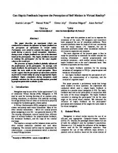
Figure B–IV.1: Formal meaning of the dependence statement.

IV–3.1 Formal definition of dependences The following informal definition of dependences can be stated: c A signal x depends on a signal y “at” a Boolean condition c (noted y − → x) if, at each instant for which c is present and true, the event setting a value to x cannot precede the event setting a value to y. A formal definition in the form of an automaton is presented here. We give the formal meaning of the statement c y− →x

(IV.1)

in Figure B–IV.1. In the figure, the clock equations in states can be read as follows: y 2 (c + c2 ) = 0 means “absent(y) ∨ (absent(c) ∨ c = f alse)” (at the considered instant); y 2 = 0 means “absent(y)”; c + c2 = 0 means “(absent(c) ∨ c = f alse)”. This figure describes a non deterministic automaton which represents the legal schedulings of calculi in one instant as conform with statement (IV.1). • States of the automaton are made of dependence graphs and clock equations. Clock equations can be represented as equations in F3 . • Transitions are labelled by signals (y, c, x), or by the empty word ε. A transition labelled by y reads: “signal y occurs, with any legal value”. A transition labelled by c(1) (respectively, c(−1))

IV–3. DEPENDENCES

61

reads: “signal c occurs, with value true (respectively, false)”; the empty word ε represents the occurrence of any signal but (y, c, x). • In the automaton of Figure B–IV.1, all the states have an additional transition (not represented in the Figure), labelled by ε, toward the initial state (which is represented with a thick circle in the Figure). The automaton describing all legal schedulings of calculi for a program in one instant is obtained by a synchronous product of such basic automata, as described in section IV–3.3. Since these automata describe instantaneous behaviors, they are called micro automata. The states of the transition system describing the overall behavior of a program are the forced states (or initial states) of the micro automata.

IV–3.2 Implicit dependences The equations defining a process may induce implicit dependences, such as described in the following. Notations: For a Boolean c, we use the notation [c] to represent the clock at which c has the value true, and [¬c] to represent the clock at which c has the value f alse. In addition to the implicit dependences described below, the following implicit dependences apply equally: bx • for any signal x, bx −−→ x bc bc • for any Boolean signal c, c −→ [c] and c −→ [¬c] [c] c • any dependence y − → x implies implicitly a dependence [c] −−→ x.

2-a Monochronous definitions • Definitions by extension: b :=: f (a1 , . . . , an ) The following implicit dependences exist: a1 − → b, . . . , an − →b • Clock: b :=:ba b is identified with the clock of a, there is no implicit dependence. • Delay: b :=: a $ init v There is no implicit dependence.

2-b Polychronous definitions • Extraction: b :=: a1 when a2 The following implicit dependences exist: bb a1 −→ b bb a2 −→bb


62 • Merging:

b :=: a1 default a2 The following implicit dependences exist: ba1 a1 −−→ b ba2 b− ba1 a2 −−−−−−−→ b whereba2 b−ba1 designates the clock representing the instants of a2 that are not instants of a1 .

IV–3.3 Micro automata 3-a Definition of micro automata The micro automaton associated with a program describes the legal schedulings of calculi in one instant. Let A be a set of variables; As = A+ ∪ A− is the set of variables of A labelled by + or −. A word on A is any subset m of As such that as ∈ m ⇒ as 6∈ m where + = − and − = + A micro automaton on A is a tuple < S, P(As ), SI , Γ ⊂ S × P(As ) × S > such that: • SI ⊂ S: S is the set of states and SI is a set of initial states; m

m

• if s1 ;1 s2 ∈ Γ (Γ is the set of transitions, m1 is the label of the transition), and s2 ;2 s3 ∈ Γ, and m . . . and sn ;n sn+1 ∈ Γ, then: ∀i 6= j, mi ∩ mj = ∅ n [ and m = mi is a word on A. i=1 ∅

• if s1 ; s2 ∈ Γ

then

s 2 ∈ SI

1

The micro automaton is said saturated if, in addition, m

m

s1 ;1 s2 ∈ Γ and s2 ;2 s3 ∈ Γ ⇒ s1

m1 ∪m2

;

s3 ∈ Γ

Let AU T be a micro automaton, Sat(AU T ) is the saturated micro automaton which contains AU T . Consider two micro automata defined respectively on A1 and A2 with A1 ∩ A2 = A. Two labels of transitions, m1 on A1 , and m2 on A2 , are said to coincide on A if and only if: (m1 ∩ As ) = (m2 ∩ As ) Let AU T1 =< S1 , P(As1 ), S1I , Γ1 > and AU T2 =< S2 , P(As2 ), S2I , Γ2 > two micro automata. Their product, denoted AU T = AU T1 ||AU T2 , is the micro automaton on A1 ∪ A2 , defined by: AU T = Sat(< S1 × S2 , P(As1 ∪ As2 ), S1I × S2I , Γ >) 1

∅ is denoted ε in IV–3.1.

IV–3. DEPENDENCES

63

with Γ defined as follows: m

m

(s1 , s2 ) ;1 (s01 , s2 ) ∈ Γ m (s1 , s2 ) ;2 (s1 , s02 ) ∈ Γ m ∪m (s1 , s2 ) 1; 2 (s01 , s02 ) ∈ Γ

iff m1 ∩ As2 = ∅ and s1 ;1 s01 ∈ Γ1 m iff m2 ∩ As1 = ∅ and s2 ;2 s02 ∈ Γ2 iff m1 and m2 coincide on A1 ∩ A2 m m and s1 ;1 s01 ∈ Γ1 and s2 ;2 s02 ∈ Γ2

3-b Construction of basic micro automata (i) Micro automaton associated with a system of equations Let us consider a system of equations on a set of variables A: Σ : R(A) = 0 having at least one solution (the system encodes clock equations of a program). A partial valuation of Σ is any system of equations Σ0 : R0 (A0 ) = 0 equivalent to R(A) = 0 in which a non empty subset {a1 , . . . , an } of variables of A have been replaced by values v1 , . . . , vn ∈ {−1, 1} such that Σ0 has at least one solution. If σ denotes such a substitution, the following notations are used: σ(ai ) = vi denotes the value assigned to ai by σ σ(R(A)) denotes the system R0 (A0 ) obtained by the substitution. Then we consider P(Σ) the set of R0 (A0 ) such that there exists σ verifying σ(R(A)) = R0 (A0 ). The micro automaton associated with Σ is the saturated micro automaton < S, P(As ), {s0 }, Γ > such that: • there exists a bijection φ : P(Σ) → S with φ(R) = s0 • for any valuation σ of R0 (A0 ) ∈ P(R(A)), φ(R0 ) ; φ(σ(R0 )) ∈ Γ T

if and only if: a+ ∈ T a− ∈ T

iff σ(a) = 1 and iff σ(a) = −1

• for all Σ0 : R0 (A0 ) = 0 such that ∀a, a ∈ A0 ⇒ a = 0 is a solution of Σ0 then

∅

φ(R0 ) ; s0 ∈ Γ

64


(ii) Micro automaton associated with a dependence The micro automaton associated with

c y− →x

is defined as follows. We consider the following states of resolution E: c y− → x, y − → x, {y, x}, {c, x}, (y 2 (c + c2 ) = 0), {y}, {x}, {c}, (c + c2 = 0), (y 2 = 0) c The micro automaton associated with y − → x is the saturated micro automaton Sat(< S, P({y, x, c}s ), {s0 }, Γ >) c

such that there exists a bijection φ : E → S with φ(y → x) = s0 and with Γ defined as follows: c c+ φ(y − → x) ; φ(y − → x) ∈ Γ c c− → x) ; φ({y, x}) ∈ Γ φ(y − y± c φ(y − → x) ; φ({c, x}) ∈ Γ c x± φ(y − → x) ; φ(y 2 (c + c2 ) = 0) ∈ Γ c ∅ c φ(y − → x) ; φ(y − → x) ∈ Γ y±

φ(y − → x) ; φ({x}) ∈ Γ x±

φ(y − → x) ; φ(y 2 = 0) ∈ Γ ∅ c φ(y − → x) ; φ(y − → x) ∈ Γ In addition, Γ contains all other transitions providing from resolutions such as described in (i). The corresponding micro automaton is displayed in Figure B–IV.1, where c+ and c− are denoted respectively c(1) and c(−1), and y ± and x± are denoted y and x; moreover, the ∅ transitions have been omitted in the figure. The complete micro automaton is the saturated micro automaton which contains this one.

(iii) Micro automaton associated with a memorization The encoding presented in IV–3.1 considers not only the clocks, but also the values of the Boolean flows: delayed Boolean flows are the state variables of the program. The micro automaton associated with x :=: y $ init v where x and y are Boolean flows is the saturated micro automaton obtained from the micro automaton depicted on Figure B–IV.2. The initial states of this micro automaton are the states represented with a thick circle in the Figure.

(iv) Micro automaton associated with a process The micro automaton associated with a process is the product of the micro automata associated with each definition involved in the process.

IV–3. DEPENDENCES

65

φ

φ

x :=: y$ init true

x :=: y$ init false

y(−1) x(1)

y(1)

y(1)

y(−1)

φ

x(−1)

y(−1) y(1)

x(1)

x(1)

x(−1)

x(−1)

φ

Figure B–IV.2: Micro automaton of x :=: y $ init v

Part C

THE SIGNALS

Chapter V

Domains of values of the signals A signal is a sequence of values associated with a clock. These values have all the same type, which is considered as the type of the sequence. The objective of this chapter is to present the notations used to represent these types and the processings which are applied on them. An element of the set of types of the S IGNAL language is denoted type. Let E be a term of the S IGNAL language; we denote by τ (E) the type associated with the term E and, when E is a constant expression, ϕ(E) the value of this expression, elaborated in the context in which E appears. The set of types of the S IGNAL language contains the scalar types, the external types, the array types and the tuple types. 1. Context-free syntax SIGNAL-TYPE ::= Scalar-type | | | |

External-type ENUMERATED-TYPE ARRAY-TYPE TUPLE-TYPE

V–1 Scalar types Scalar types are the following: synchronization types, integer types, real types, complex types, character type, string type; the integer, real and complex types compose the set of numeric types; character and string types compose the set of alphabetic types. 1. Context-free syntax Scalar-type ::= Synchronization-type | Numeric-type | Alphabetic-type

Numeric-type ::= Integer-type | Real-type | Complex-type

Alphabetic-type ::=

char | string

DOMAINS OF VALUES OF THE SIGNALS

70

V–1.1 Synchronization types The synchronization types are used to define the clocks of the signals. They are the type event (or pure signal) and the type boolean.

Denotations of types 1. Context-free syntax Synchronization-type ::=

event | boolean

2. Types (a) (b)

τ (event) = event τ (boolean) = boolean

Denotations of values • A signal of type event takes its values in a single-element set: there is no associated constant and a parameter cannot be of that type. • The constants of type boolean are the logical values denoted with the syntax of a Boolean-cst (cf. part A, section II–2.2, page 23). • The default initial value of type boolean is the value f alse.

V–1.2 Integer types Integer values can be in short representation (type short), normal representation (type integer), or long representation (type long); a given implementation may not distinguish these types. In this document, the notations max long, min long, max integer, min integer, max short and min short will be used to designate respectively: the greatest representable integer (of type long), the smallest representable integer (of type long), the greatest integer of type integer, the smallest integer of type integer, the greatest integer of type short and the smallest integer of type short. These values depend of the implementation and respect the following order: min long ≤ min integer ≤ min short ≤ 0 < max short ≤ max integer ≤ max long min integer < 0

Denotations of types 1. Context-free syntax Integer-type ::=

short | integer | long

2. Types (a)

τ (short) = short

V–1. SCALAR TYPES (b) (c)

71

τ (integer) = integer τ (long) = long

Denotations of values The positive values of an integer type are denoted following the syntax of an Integer-cst (cf. part A, section II–2.3, page 24). A negative value has not a direct representation: it is obtained using the operator − applied to a positive value. 1. Types (a) The type of an Integer-cst E is the smallest integer type that contains it. 2. Semantics • An Integer-cst denotes an integer value represented in decimal base, contained between 0 and max long. • An occurrence of an integer value of type short (respectively, integer and long) smaller than min short (respectively, min integer and min long) or greater than max short (respectively, max integer and max long) results, in the considered type, in a value depending of the implementation. • For an Integer-type, the default initial value is the value 0.

Bounded integers Integers have a special role since they can be used to index arrays. In that case, we have to consider bounded values. In this document, for a given signal E, we will use sometimes the following notations: • lower_bound(E) designates the lower bound of the values of E; • upper_bound(E) designates the upper bound of the values of E. These bounds are constant integers.

V–1.3 Real types The real values can be in simple precision representation (type real) or double precision representation (type dreal); a given implementation may not distinguish these types.

Denotations of types 1. Context-free syntax Real-type ::=

real | dreal

2. Types (a) (b)

τ (real) = real τ (dreal) = dreal


72

Denotations of values E1 .E2 eE3 (simple precision) or E1 .E2 dE3 (double precision) A value of real type is denoted following the syntax of a Real-cst (cf. part A, section II–2.4, page 24). A Real-cst denotes the approximate value of a real number. 1. Types (a) A Simple-precision-real-cst is of type real. (b) A Double-precision-real-cst is of type dreal. 2. Semantics • The value ϕ(Ei ), when Ei is omitted, is 0. • If E2 has n digits, the value of the constant is the approximate value of (ϕ(E1 ) + ϕ(E2 ) ∗ 10−n ) ∗ 10ϕ(E3 ) . • For a Real-type, the default initial value is the value 0.0 or 0.0d0 following the type.

V–1.4 Complex types The complex values have the common representation of their components (simple or double precision, respectively types complex and dcomplex); both types are distinguished in a given implementation if and only if the type dreal is distinguished from the type real.

Denotations of types 1. Context-free syntax Complex-type ::=

complex | dcomplex

2. Types (a) (b)

τ (complex) = complex τ (dcomplex) = dcomplex

Denotations of values A value of complex type is obtained for example in the following expression, the first element of which is the real part and the second one the imaginary part (cf. part C, section VI–8.1, page 128). 1. Examples (a) 1.0 @ (−1.0) For a Complex-type, the default initial value is the pair of default real initial values.

V–2. EXTERNAL TYPES

73

V–1.5 Character type The type character contains the set of the admitted characters in the language.

Denotation of type 1. Types (a)

τ (char) = character

Denotations of values A value of type character is denoted by a Character-cst (cf. part A, section II–2.5, page 24). The default initial value of type character is the character ’\000’.

V–1.6 String type The type string allows to represent any sequence of admitted characters. The value of the maximal authorized size for a string, maxStringLength, depends of the implementation.

Denotation of type 1. Types (a)

τ (string) = string

Denotations of values A value of type string is denoted by a String-cst (cf. part A, section II–2.6, page 25). The default initial value of type string is the empty string "".

V–2 External types External types make possible the use of signals the type of which is not a type of the language.

Denotation of type A An external type is designated by a name. 1. Context-free syntax External-type ::= Name-type 2. Types (a) For an external type with name A, τ (A) = A Two external types with distinct names are not comparable. 3. Examples (a) pointer is an external type with name pointer.


74

Denotations of values An external constant can be denoted by a name; the value of an external constant can be defined by the environment of the program (cf. part E, chapter XII, page 191). For example the identifier nil can represent a constant of type pointer. For any external type A, it is possible to define a constant that represents the default initial value of type A (cf. section V–7, page 84). The only operations the semantics of which is defined on external type signals are operations of description of communication graphs (which are polymorphic operations).

V–3 Enumerated types Enumerated types allow to represent finite domains of values represented by distinct names. These values (the enumerated values) are the constants of the type to which they belong.

Denotation of types enum (a1 , ..., am ) An enumerated type is defined by the list (considered as an ordered list) of its values (the enumerated values) and by its name (cf. section V–7, page 84): type A = enum (a1 , ..., am ); However, like for the other types, such a name does not necessarily exist. In that case, the name of the type is empty. The definition of an enumerated type declares its enumerated values. 1. Context-free syntax ENUMERATED-TYPE ::= enum

(

Name-enum-value { , Name-enum-value }∗

)

2. Types (a) The type of the enumerated type is: τ (A = enum (a1 , ..., am )) = A × {a1 , . . . , am } where {a1 , . . . , am } represents the finite set of ordered values a1 , . . . , am . It means that the name of an enumerated type (the name that is given in the declaration of the type) is part of that type. Depending on the implementation, it can be the case or not that synonyms (cf. section V–7, page 84) are considered in the definition of the type. If the enumerated type is not designated by a name, then its type is just the finite set of its ordered values. (b) The type of the enumerated values of an enumerated type is this enumerated type: . . . = τ (am ) = τ (enum (a1 , ..., am ))

τ (a1 ) =

(c) Two enumerated types are considered to be equal if they have both the same name, and the same set of enumerated values, in the same order. Two enumerated types that are not designated by a name are considered to be equal if they have the same set of enumerated values, in the same order. 3. Semantics The enumerated values of an enumerated type are ordered (syntactic order of their declaration). All the values of a given type are distinct; these values are distinguished by their name.

V–4. ARRAY TYPES

75

4. Examples (a) type color = enum (yellow, orange); and type fruit = enum (apple, orange); are two enumerated types, each one defining an enumerated value named “orange”. Both enumerated values named “orange” are distinct values, with different types. The next paragraph describes the way allowing to distinguish them.

Denotation of values #ai or A#ai where A is the name of the enumerated type. Note: the symbol # does not appear in the definition of the type (and its enumerated values), but only for the use of an enumerated value. 1. Context-free syntax ENUM-CST ::= # Name-enum-value | Name-type # Name-enum-value

2. Semantics • The notation #ai can be used to reference an enumerated value ai in a context in which there is no possible ambiguity on the referenced value. If it is not the case, the notation A#ai has to be used, where A designates the enumerated type. • The default initial value of an enumerated type is the first value of its declaration. 3. Clocks An enumerated value ai (designated by #ai or A#ai ) is a constant. (a)

ω(ai ) = ~

4. Examples (a) color#orange and fruit#orange designate two different enumerated values (of two different types) with the same name.

V–4 Array types An array is a structure allowing to group together synchronous elements of a same type. The description of such a structure and of the access to its elements uses constant expressions that have the general syntax of signal expressions (S-EXPR).

Denotation of types [n1, ..., nm ]ν An array type is defined by its dimensions and by the type of its elements. 1. Context-free syntax


76 ARRAY-TYPE ::= [

S-EXPR { , S-EXPR }∗

] SIGNAL-TYPE

2. Types (a) The elaborated values of n1 (ϕ(n1 )), . . . , nm (ϕ(nm )) are strictly positive integers. (b) The type of the array is: τ ([n1 , ..., nm]ν ) = ([0..ϕ(n1 ) − 1] × . . . × [0..ϕ(nm) − 1]) → τ (ν ).

(c) When the type τ (ν ) itself is an array type [nm+1 , ..., nm+p ]µ, then the type of the array is: τ ([n1 , ..., nm]ν ) = ([0..ϕ(n1 ) − 1] × . . . × [0..ϕ(nm+p) − 1]) → τ (µ).

3. Clocks The integers ni must be constant expressions. (a)

ω(ni ) = ~

4. Properties (a) The types [n1 , n2 ]ν and [n1 ] [n2 ]ν are the same. 5. Examples (a) [10,10] integer is a two dimensions integer array (the bounds of the array begin implicitly at index 0 in each dimension). (b) [n] pointer is a vector of values of external type pointer.

Denotations of values A constant array is defined by a constant expression of array (cf. part D, section IX–2, page 149); the elements that compose a constant array are from the same domain. For an ARRAY-TYPE, the default initial value is an array of which each element has the default initial value of the type of the elements of the array.

V–5 Tuple types The S IGNAL language allows to define structured types, called in a generic way tuple types. Two categories of tuple types, called also tuple types with named fields, can be associated with the objects of the S IGNAL language in declarations: • polychronous tuples (designated by the keyword bundle)1; • monochronous tuples (designated by the keyword struct) (remark: the objects declared of tuple type can also be called tuples). An object declared of type polychronous tuple is in fact a gathering of objects (family of objects). In this way, a polychronous tuple of signals is not a signal (for example, in the general case, it has no clock); it cannot be used as the type of the elements of an array. At the opposite, an object declared of 1

not yet implemented in P OLYCHRONY: clock properties of bundles are not taken into account.

not yet fully implemented

V–5. TUPLE TYPES

77

type monochronous tuple can be a signal: it has a clock (delivered by the operator b) and it can be used as the type of the elements of an array. A general rule is that operators on signals do not apply on polychronous tuples, but they are pointwise extended on the fields of these tuples (cf. part D, chapter X, page 169). The S IGNAL language allows also to manipulate gatherings (or tuples) of objects with no explicit declaration of these gatherings. They define in fact tuples with unnamed fields, the type of which is a product of types (cf. section V–6.2, paragraph “Order on tuples”, page 80). The operators defined on signals are pointwise extended to tuples with unnamed fields (cf. part D, chapter X, page 169). By extension, it will be possible to refer to the clock of a tuple of signals if all the signals of the tuple have the same clock.

Denotation of types struct (µ1 X1 ; ...; µm Xm ;) or bundle (µ1 X1 ; ...; µm Xm ;) spec C A tuple type is defined by a list of typed and named fields; in addition, clock properties can be specified on the fields of a tuple. The description of such a type uses lists of declarations of sequence identifiers S-DECLARATION (cf. section V–9, page 87) for the designation of the fields, and properties SPECIFICATION-OFPROPERTIES (cf. part E, section XI–6, page 180) to express the clock properties that must be respected by the signals corresponding to the fields defined by the type. These properties should describe exclusively clock properties on the fields of the tuple, excluding for instance graph properties. Note that constraints on values can be specified under the form of constraints on clocks. A tuple type can be multi-clock (polychronous) or mono-clock (monochronous). If it is multi-clock, it is distinguished by the keyword bundle and it can contain specifications of clock properties applying on its fields. If it is mono-clock, it is distinguished by the keyword struct and all its fields are implicitly synchronous; in this case, it can be used as type of the elements of an array. 1. Context-free syntax TUPLE-TYPE ::= struct

( NAMED-FIELDS )

| bundle ( NAMED-FIELDS ) [ SPECIFICATION-OF-PROPERTIES ]

NAMED-FIELDS ::= { S-DECLARATION }+

2. Types (a) From the point of view of the domains of associated values, the polychronous or monochronous tuple types with named fields are designated in the same way in this document. The domain is a non associative product (i.e., preserving the structuring) of typed named fields. (b)

τ (struct

(c)

τ (bundle

(µ1 X1 ; ...; µm Xm ;)) = bundle({X1 } → τ (µ1 ) × . . . × {Xm } → τ (µm )) (µ1 X1 ; ...; µm Xm ;) spec C ) = bundle({X1 } → τ (µ1 ) × . . . × {Xm } → τ (µm ))


78

(d) A type bundle({X1 } → τ (µ1 ) × . . . × {Xm } → τ (µm )) defines a set of functions m [ Ξ : {X1 , . . . , Xm } → τ (µi ) such that Ξ(Xi ) ∈ τ (µi ). i=1

3. Semantics The tuple types with named fields (struct and bundle) allow to define structured types as non associative grouping of typed named fields: (µ1 X1 ; ...; µm Xm ;). The specifications of properties spec C apply on the fields of the tuple. They establish constraints that must be respected by the signals defined with such a type (space of synchronization of the values of the domain). 4. Examples (a) struct (integer X1, X2;) is a tuple of two synchronous integers. (b) bundle (integer A; boolean B;) spec (| A b# B |) defines a union of types as a tuple the fields of which are mutually exclusive.

Denotations of values A constant tuple is defined by a constant expression of tuple (cf. part D, section VIII–1, page 143). For a TUPLE-TYPE, the default initial value is recursively the tuple of initial values of its fields.

V–6 Structure of the set of types A partial order is defined on the types such that there exists a “natural” plunging of a smaller set into a greater one. The types are organized into domains corresponding to theoretical sets (non constrained by the implementation). In this way, the domain of synchronization values (Synchronization-type) contains the types event and boolean; the domain of integers (Integer-type) contains the types short, integer, and long; the domain of reals (Real-type) contains the types real and dreal; the domain of complex (Complex-type) contains the types complex and dcomplex.

V–6.1 Set of types The set of types is composed of the types the expressions of which, in the S IGNAL language, described in the following summary, are derived from the variable SIGNAL-TYPE:

V–6. STRUCTURE OF THE SET OF TYPES

79

SIGNAL-TYPE  Scalar-type      Synchronization-type       (    event denotes the type event            boolean denotes the type boolean         Numeric-type          Integer-type                     short denotes the type short                     integer denotes the type integer           long denotes the type long            Real-type  (       real denotes the type real                 dreal denotes the type dreal              Complex-type       (          complex denotes the type complex              dcomplex denotes the type dcomplex         Alphabetic-type   (     char denotes the type character          string denotes the type string      External-type     Name-type     Generic form of the external types: name     ENUMERATED-TYPE      enum ( Name-enum-value { , Name-enum-value }∗ )      Generic form of the enumerated types: A × {a1 , . . . , am }     ARRAY-TYPE     [ S-EXPR { , S-EXPR }∗ ] SIGNAL-TYPE      Generic form of the array types: ([0..n1 − 1] × . . . × [0..nm − 1]) → ν     TUPLE-TYPE        struct ( NAMED-FIELDS )         bundle ( NAMED-FIELDS ) [ SPECIFICATION-OF-PROPERTIES ]       Generic form of the tuple types with named fields:      bundle({X1 } → µ1 × . . . × {Xm } → µm )

V–6.2 Order on types Order on scalar and external types

→

The order on scalar and external types of the S IGNAL language is described in the figure C–V.1. A downward solid arrow ( ) links a type with a type directly superior from the same domain (two types of a same domain are comparable); the other arrows represent basic conversions, the semantics of which is described below. The other conversions are obtained by composition of conversions. The partial order is denoted v. The notion of “comparable types” is extended to arrays and tuples.


80

event

EXTERNAL_TYPE boolean

string

short real

complex

dreal

dcomplex

integer char long

Figure C–V.1: Order and conversions on scalar and external types

Order on arrays The order on scalar and external types is extended to arrays: • ([0..m1 − 1] × . . . × [0..mk − 1]) → µ v ([0..n1 − 1] × . . . × [0..nl − 1]) → ν if and only if ∗ k=l ∗ ∀i 1 ≤ i ≤ k ⇒ mi ≤ ni ∗ and µ v ν

Order on tuples A product of types is a type, called tuple type with unnamed fields, which preserves the structuring. There is no syntactic designation of such a type (it is not possible to declare some object of type tuple with unnamed fields); however, it is possible to manipulate objects of type tuple with unnamed fields (product of types). A tuple with unnamed fields with a single element is considered as isomorphic to this element. The product of types µ1 , . . . , µn (in this order) is denoted (µ1 × . . . × µn ). The order on the types of signals is extended as follows on tuples:


81

• bundle({X1 } → µ1 × . . . × {Xn } → µn ) v bundle({Y1 } → ν1 × . . . × {Yp } → νp ) if and only if: p=n and (∀ i) ( Xi = Yi et µi v νi ) • (µ1 × . . . × µn ) v bundle({Y1 } → ν1 × . . . × {Yp } → νp ) if and only if: (µ1 × . . . × µn ) v (ν1 × . . . × νp ) • (µ1 × . . . × µn ) v (µ1 × (µ2 × . . . × µn )) • (µ1 × . . . × µn ) v (ν1 × . . . × νp ) if and only if: V ((n = p) ( (∀i) ( µi v νi ) )) or (V(∃k, l) ( ((i < k) ⇒ (µi v νi )) µk+l ) v νk ) V (((µk × . . . × V (((k + l = n) (kV = p)) V or (((k + l < n) (k < p)) ((µk+l+1 × . . . × µn ) v (νk+1 × . . . × νp ))))) ) )

Notation The notation µ t ν is used to designate the upper bound of two comparable types µ and ν.

V–6.3 Conversions A conversion is a function for which the image of an object of the type µ of the argument is an object of the type ν required by the context of utilization. The conversion functions for the types defined in the S IGNAL language have the name of the reserved designation of the expected type or in general the name of the expected type. In this document, these functions are denoted as follows, in order to describe their semantics: Cνµ : µ → ν Direct conversion functions are available in the language, even if their semantics is described in terms of composition of conversions.

3-a Conversions between comparable types Between two directly comparable types µ v ν, the two following conversions are defined: 1. the conversion Cνµ from a smaller type µ to a greater type ν lets the values unchanged; 2. the conversion Cµν : ν → µ which is the inverse of the previous one for the values of type µ.

The conversion functions are extended to any pair of comparable types: • if ν1 v µ v ν2 then Cνν21 = Cνµ2 ◦ Cµν1 ; • Cµµ is the identity function.

Implicit conversions The only implicit conversions are the conversions Cνµ for which µ v ν. Implicit conversions do not need to be explicited in the language.


82

3-b Conversions toward the domain “Synchronization-type” µ The conversions Cevent are defined for each µ (except if µ is a polychronous tuple); Trivially, they

deliver the single value of type event. µ the conversions Cboolean depend of the implementation while respecting the following rules: long • The conversion Cboolean verifies: long – Cboolean (0) = f alse long – Cboolean (1) = true

• For a Scalar-type µ distinct from event µ long µ Cboolean = Cboolean ◦ Clong

3-c

Conversions toward the domain “Integer-type”

µ The conversions Cshort depend of the implementation while respecting the following rules: integer • Cshort (v) = v if v is greater than min short and smaller than max short (non strictly in both cases), long integer long • Cshort = Cshort ◦ Cinteger

• for a Scalar-type or ENUMERATED-TYPE µ µ long µ Cshort = Cshort ◦ Clong µ The conversions Cinteger depend of the implementation while respecting the following rules: long • Cinteger (v) = v if v is greater than min integer and smaller than max integer (non strictly in both cases),

• for a Scalar-type µ which is not smaller than integer (for the order defined on the types), or for µ an ENUMERATED-TYPE µ long µ Cinteger = Cinteger ◦ Clong µ The conversions Clong depend of the implementation while respecting the following rules: boolean is defined by the following rules: • the conversion Clong boolean (f alse) = 0 – Clong boolean (true) = 1 – Clong character (C) is the numerical value of the code of the character C, • the value of Clong dreal (v) is the integer part n of v if n is greater than min long and smaller than • the value of Clong max long (non strictly in both cases),

• for a Scalar-type µ which is not smaller than long (for the order defined on the types) µ dreal ◦ C µ Clong = Clong dreal µ • for an ENUMERATED-TYPE µ equal to A × {a1 , . . . , am }, the conversion Clong is defined by: µ µ Clong (a1 ) = 0, . . . , Clong (am ) = m − 1.


83

3-d Conversions toward the domain “Real-type” For each Real-type, a given implementation distinguihes the safe numbers (in the same sense as in Ada), which have an exact representation. µ The conversions Creal depend of the implementation while respecting the following rules: dreal (v) = v • if v, of type dreal, is a safe number in the type real, Creal

• the conversion preserves the order on the real numbers included between the smallest and the greatest safe number in the type real, • for a Scalar-type µ µ dreal ◦ C µ Creal = Creal dreal µ The conversions Cdreal depend on the implementation while respecting the following rules:

• the conversion preserves the order on the real numbers included between the smallest and the greatest safe number in the type dreal, dcomplex • Cdreal (re@im) = re complex dcomplex complex • Cdreal = Cdreal ◦ Cdcomplex long • if v, of type long, is a safe number in the type dreal, Cdreal (C) = v

• for a Scalar-type distinct of the previous ones, µ long µ Cdreal = Cdreal ◦ Clong

3-e

Conversions toward the domain “Complex-type”

There are no conversions toward the domain Complex-type except those internal to that domain. However, a given implementation can provide such conversion functions. Note that the conversion of a real re into a complex (respectively, of a dreal re into a dcomplex) can be obtained by [email protected]. dcomplex The conversion Ccomplex depends on the implementation while respecting the following rule: dcomplex dreal (re), C dreal (im)} • Ccomplex (re@im) = {Creal real

3-f

Conversions toward the types character and string

µ depend on the implementation while respecting the following rules: The conversions Ccharacter long • the value of Ccharacter (v) is the character (if it exists) whose decimal value of its code is equal to v, µ long µ • for a Scalar-type µ Ccharacter = Ccharacter ◦ Clong

There is no conversion toward the type string.


84

3-g Conversions of arrays For any tuple of strictly positive integers n1 , . . . , nm , and any conversion Cνµ , ([0..n − 1] × . . . × [0..nm − 1]) → µ the conversion C([0..n11 − 1] × . . . × [0..nm − 1]) → ν is defined by: ([0..n − 1] × . . . × [0..n

− 1]) → µ

µ m C([0..n11 − 1] × . . . × [0..nm − 1]) → ν (T ) = Cν ◦ T

3-h Conversions of tuples Conversions of tuples with unnamed fields For any conversions Cνµ11 , . . . , Cνµnn , (µ × . . . × µ ) the conversion C(ν11 × . . . × νnn) is defined by: (µ × . . . × µ )

C(ν11 × . . . × νnn) (x1 , . . . , xn ) = (Cνµ11 (x1 ), . . . , Cνµnn (xn ))

Conversions of tuples with unnamed fields toward tuples with named fields For any conversions Cνµ11 , . . . , Cνµnn and any tuple with named fields of type bundle({X1 } → ν1 × . . . × {Xm } → νm ) that defines a function Ξ (cf. section V–5, page 76), (µ1 × . . . × µn ) the conversion Cbundle({X is defined by: 1 } → ν1 × . . . × {Xm } → νm ) (µ × . . . × µ )

(µ × . . . × µ )

n 1 Cbundle({X = Ξ ◦ C(ν11 × . . . × νnn) 1 } → ν1 × . . . × {Xm } → νm )

V–7 Denotation of types A type can be designated by an identifier, declared in a DECLARATION-OF-TYPES (it cannot be an identifier of predefined type). In particular, such a type identifier can designate a generic type, which can represent a type of the language or an external type.

Denotation of type A 1. Context-free syntax SIGNAL-TYPE ::= Name-type

2. Types (a) The type designated by a Name-type A is the type associated with A in the declaration of the type A.

Declarations of types type A = µ; type A;

or

1. Context-free syntax DECLARATION-OF-TYPES ::= type DEFINITION-OF-TYPE { , DEFINITION-OF-TYPE }∗

;

V–8. DECLARATIONS OF CONSTANT IDENTIFIERS

85

DEFINITION-OF-TYPE ::= Name-type | Name-type = DESCRIPTION-OF-TYPE

DESCRIPTION-OF-TYPE ::= SIGNAL-TYPE | EXTERNAL-NOTATION [ TYPE-INITIAL-VALUE ]

TYPE-INITIAL-VALUE ::= init Name-constant

2. Types (a) The declaration type A = µ; defines the type A as being equal to the type µ: τ (A) = τ (µ) (b) When it appears in the formal parameters of a model (cf. part E, section XI–5, page 179), the declaration type A; defines a formal generic type whose actual value is provided within the call of the model (cf. section VI–1.2, page 97). Otherwise, the declaration type A; is an abbreviated form for type A = external; that specifies A as an externally defined type. It means that A is either an external type the actual definition of which is provided in the environment of the program, or it is a formal generic type, whose actual value is defined elsewhere in the context or is provided in a module (cf. part E, section XII–1, page 191). It is possible to specify, in the declaration of an external type A, a constant name (which must be the name of an external constant of type A—cf. section V–8, page 85), that allows to designate the default initial value of that type. A given compiler may consider that such a constant name appearing as default initial value of an external type constitutes an implicit declaration of this external constant. (c) If A is defined as an external type, then: τ (A) = A (d) Two external types with distinct names A and B are considered as different types. 3. Properties (a) With the declarations type A = µ; and type B = µ; then τ (A) = τ (B ) = τ (µ). Some implementations may not ensure this property. 4. Examples (a) type T = [n] integer; declares the type T as vector of integers, of size n.

V–8 Declarations of constant identifiers constant µ X1 = E1 , . . . , Yj , . . . , Xn = En ;


86

A constant sequence is a sequence each element of which has the same value. Such a sequence can be designated by an identifier. 1. Context-free syntax DECLARATION-OF-CONSTANTS ::= constant SIGNAL-TYPE DEFINITION-OF-CONSTANT { , DEFINITION-OF-CONSTANT }∗

;

DEFINITION-OF-CONSTANT ::= Name-constant | Name-constant = DESCRIPTION-OF-CONSTANT

DESCRIPTION-OF-CONSTANT ::= S-EXPR | EXTERNAL-NOTATION

2. Types (a) (∀ i) ( τ (µ) = τ (Xi ) ) (b) (∀ i) ( τ (Ei ) v τ (Xi ) ) (c) When the constant declaration does not contain an expression, for example for Yj , it is in fact an abbreviated form for Yj = external; that defines Yj as an externally defined constant. It means that the value of Yj is provided either in a module (cf. part E, section XII–1, page 191), or in the environment of the program. 3. Semantics • Any expression defining a constant must be monochronous and functional (without side effect). With this reserve, the set of expressions admitted by a compiler contains the operators and intrinsic functions and can contain a set of functions depending of a particular environment. • The elaboration of the expression Ei , in the context CD of the declaration D, minus the identifier Xi , provides a constant value (determined at compile time) ϕ(Ei ) = v; • the declaration D hides any higher declaration of Xi for the context CD and the included contexts; • in a context where D is visible, the elaboration of an occurrence of the identifier Xi provides the value ϕ(Xi ) = v. 4. Clocks An occurrence of use of Xi (or Yj ) is considered as an occurrence of the designated constant. (a) (b) (c)

ω(Ei ) = ~ ω(Xi ) = ~ ω(Yj ) = ~

V–9. DECLARATIONS OF SEQUENCE IDENTIFIERS

87

5. Examples (a) The declaration constant real PI = 3.14; defines the identifier PI of type real and with value ϕ(3.14). (b) The declaration constant [2,2] real UNIT = [[1.0,0.0],[0.0,1.0]]; defines the identifier UNIT as a unit real matrix. (c) The declaration constant RECTANGLE BASE; where RECTANGLE is an identifier of external type, defines a constant of that type: BASE, the value of which should be provided at code generation. (d) The declaration constant integer L = M + N; is incorrect if M or N does not designate a constant or a parameter; if it is correct, it defines the identifier L as being equal to the sum of the constants ϕ(M) and ϕ(N).

V–9 Declarations of sequence identifiers µ ID1 , ..., IDj init Vj , ..., IDn ; A sequence of values is provided with a type (the one of its elements); this type is associated with an identifier in a declaration. In such a declaration, an identifier can designate a static parameter (formal “signal”), a signal, or a tuple of signals. Initialization values can be associated with signals and tuples of signals (IDj init Vj ) in order to define their initial value(s) when these initial values are not defined elsewhere. 1. Context-free syntax S-DECLARATION ::= SIGNAL-TYPE DEFINITION-OF-SEQUENCE { , DEFINITION-OF-SEQUENCE }∗

;

DEFINITION-OF-SEQUENCE ::= Name-signal | Name-signal init S-EXPR

2. Types (a) The declared names must be mutually distinct. The same type τ (µ) is given to the identifiers ID1 , . . . , IDn in the context of the declaration. (b) For a signal expression (“assignment”, passage of static parameter or positional identification) associating a value v with an identifier IDi declared with type µ, we must have τ (v ) v µ. (c) The rules applying to initial values are exactly those described in the section “Initialization expression” (cf. section VI–3.1, page 107).


88 3. Semantics

• µ ID1 , ..., IDn ; declares the sequences (signals or parameters) ID1 , . . . , IDn . If µ designates a polychronous tuple type then the identifiers ID1 , . . . , IDn designate tuples of signals (and not, strictly speaking, signals); the signals represented by these tuples are, recursively, the fields of the tuples (the fields can be themselves tuples). For example, if µ designates a tuple type with named fields bundle (µ1 X1 ; ...; µm Xm ;) ... then each tuple IDi gathers the signals (or, recursively, the tuples of signals) designated by IDi .X1 , . . . , IDi .Xm (cf. part D, section VIII–3, page 144), which have respectively the types µ1 , . . . , µm . • The semantics of an initialization expression specified in a declaration is exactly the same as that described in the section “Initialization expression” (cf. section VI–3.1, page 107). The association of an initialization with a signal declaration specifies a default initialization for the corresponding signal. It can be overloaded by the definition of that signal (in that case, it is unnecessary or only partly necessary). 4. Clocks (a) The relations on the clocks of initialization expressions are described in the section “Initialization expression” (cf. section VI–3.1, page 107). 5. Examples (a) The declaration real X, Y; declares the signals X and Y of type real. (b) The declaration [n] integer V; declares the vector of integers V, of size n.

V–10 Declarations of state variables statevar µ ID1 init V1 , ..., IDj , ..., IDn init Vn ; A state variable is a typed sequence the elements of which are present as frequently as necessary (it is available at a clock which is upper than the upper bound of the clocks of all the signals of the compilation unit in which it is declared). A state variable is defined via partial definitions the clock of which are well defined. It keeps its previous value as long as a new one is defined. It should have an initial value associated with its declaration (if it has not, it takes as initial value the default initial value of its type). A state variable can be used only in a context which defines a context clock. A state variable cannot be declared as input or output of a model of process. 1. Context-free syntax DECLARATION-OF-STATE-VARIABLES ::= statevar SIGNAL-TYPE DEFINITION-OF-SEQUENCE { , DEFINITION-OF-SEQUENCE }∗

;

2. Types (a) The declared names must be mutually distinct. The same type τ (µ) is given to the identifiers ID1 , . . . , IDn in the context of the declaration.

V–10. DECLARATIONS OF STATE VARIABLES

89

(b) For a signal expression (partial “assignment” associating a value v with an identifier IDi declared with type µ, we must have τ (v ) v µ. (c) The rules applying to initial values are exactly those described in the section “Initialization expression” (cf. section VI–3.1, page 107). 3. Semantics • statevar µ ID1 , ..., IDn ; declares the state variables ID1 , . . . , IDn . • The semantics of an initialization expression specified in a declaration is exactly the same as that described in the section “Initialization expression” (cf. section VI–3.1, page 107).

Note: The INRIA P OLYCHRONY environment allows in some cases that the type of a constant, a sequence identifier or a state variable is not provided explicitly in their declaration (the corresponding SIGNAL-TYPE is simply omitted). The corresponding type must be deduced from the context of use of the object.

Chapter VI

Expressions on signals The values associated with signals are determined by equations on signals; these equations are built by composition of sub-systems of equations (named also processes) from elementary equations. This chapter presents the expressions of definition of signals (S-EXPR). This presentation is preceded by an introduction to the expressions of composition of definitions (P-EXPR).

VI–1 Systems of equations on signals Composition of definitions of signals The equations of definition of signals can be composed by the operator | (see chapter VII, “Expressions on processes”). An expression on processes E1 | E2 defines the signals (or, equivalently, has as outputs the signals) defined in each one of its sub-expressions, and has as inputs the input signals of each one of these sub-expressions which are not outputs of the other one. The value of an input signal of a sub-expression, which is defined in the other one, is the value associated by this definition. As a signal cannot have a double complete definition, a given signal identifier representing a totally defined signal cannot be output of two sub-expressions. However, it is possible to have several partial definitions, in different sub-expressions, for a given signal (partial definitions are syntactically distinguished). An expression on processes can be parenthesized by (| on the left and by |) on the right (note the presence of the symbol | ). A given output of an expression on processes can be hidden through the operator / (see chapter VII, “Expressions on processes”). An expression on processes E1 / a1 has as outputs the outputs of E1 distinct from a1 and for inputs the inputs of E1 . The signals are defined by explicit elementary equations of DEFINITION-OF-SIGNALS, CONSTRAINTs (cf. section VI–5.3, page 121), or by referring to systems of equations declared as models of processes (INSTANCE-OF-PROCESS).

VI–1.1 Elementary equations A definition of signals allows to define a signal or a set of signals with the syntax given below. A definition of signals is an expression of processes.

EXPRESSIONS ON SIGNALS

92

1-a Equation of definition of a signal X := E 1. Context-free syntax ELEMENTARY-PROCESS ::= DEFINITION-OF-SIGNALS

DEFINITION-OF-SIGNALS ::= Name-signal := S-EXPR

2. Profile An equation of definition of a signal has as output the defined signal and as inputs the inputs of the expression E distinct of the output. • ! (X := E ) = {X} • The inputs of E are the signal identifiers that have at least one occurrence in E. ? (X := E ) = ? (E) − ! (X := E ) 3. Types (a)

τ (E ) v τ (X )

4. Semantics The signal X is equal to the signal resulting from the evaluation of E. An occurrence of X in the expression E builds a recursive definition. 5. Definition in SIGNAL Though it is the most frequently form of equation used in the S IGNAL language, X := E is not the basic form. The sign := expresses that the equation is oriented, while in the basic form (cf. part B, chapter III, page 29) the sign :=: is used to express the fact that equations are non oriented (cf. section VI–6, page 122). It is equal to the following process, where the dependences are made explicit: ( | X :=: E | E −−> X |)

6. Clocks A signal represented by an identifier and the signal that defines it are synchronous. (a)

ω(X ) = ω(E )

7. Graph (a) E − →X 8. Examples (a) if x, y, z designate signals: x := y + z defines the signal designated by x, equal to the sum of the signals designated respectively by y and z; this expression has as inputs y and z and as output x.

VI–1. SYSTEMS OF EQUATIONS ON SIGNALS

93

1-b Equation of multiple definition of signals (X1 ,. . . ,Xn) := E 1. Context-free syntax DEFINITION-OF-SIGNALS ::= (

Name-signal { , Name-signal }∗

)

:= S-EXPR

2. Profile An equation of multiple definition of signals has the inputs and outputs defined by the following rules. • The identifiers of defined signals represent the outputs of the equation: ! ((X1 ,. . . ,Xn) := E ) = {X1 , . . . , Xn } • The inputs of the equation are the inputs of E which are not outputs of the equation: ? ((X1 ,. . . ,Xn) := E ) = ? (E) − ! ((X1 ,. . . ,Xn) := E ) 3. Types (a) (b)

τ ((X1 ,. . . ,Xn)) = (τ (X1 ) × . . . × τ (Xn )) τ (E ) v (τ (X1 ) × . . . × τ (Xn ))

4. Semantics • X1 , . . . , Xn designate signals or tuples of signals. • E can be viewed as a tuple of n elements: let (E1 ,. . . ,En) this tuple. • Each signal or tuple Xi is respectively equal to the signal or tuple Ei that corresponds to it positionally as output of E. 5. Definition in SIGNAL (X1 ,. . . ,Xn) := E is equal to the following process: (|

X1 := E1 .. .

| Xn := En |) As a particular case, when the defined signal or tuple is unique, (X) := E is equivalent to: X := E (the syntax without parentheses as described in 1-a can be used when X is a tuple). 6. Clocks A signal represented by an identifier and the signal Ei that defines it are synchronous. In this case, there is: (a)

ω(Xi ) = ω(Ei )

7. Graph (a) Ei − → Xi


94 8. Examples

(a) if x, y, z, a designate signals and P a model with one formal parameter, one input and three outputs: (x,y,z) := P{ n }( a+5 ) defines the signals designated by x, y and z, equal respectively to the first, second and third output of the model P instantiated with the parameter n and taking at +5 as input at each occurrence of a; this expression has as input a and as outputs x, y and z; (b) if w, v, b also designate signals: (w,x,y,z,v) := (a,P{ n }( a+5 ),b) defines the signals w, x, y, z and v, equal respectively to the signal a, to the first, the second and the third output of the process P, and to the signal b; this expression has as inputs a and b and as outputs w, x, y, z and v; it is equivalent to the composition (| (w,v) := (a,b) | (x,y,z) := P{ n }( a+5 ) |); (c) if x designates a tuple with named fields whose fields are respectively x1 and x2, and a, b designate signals: (a,b) := (x.x1,x.x2) defines the signals a and b equal respectively to the first and the second component of the tuple x; (d) if x designates a tuple with named fields and a, b designate signals: x := (a,b) defines the tuple x the components of which are respectively equal to the signals a and b.

1-c

Equation of partial definition of a signal

Equations of partial definition of a signal are a way to avoid the syntactic single assignment rule, even if semantically, this rule applies. Each one of the partial definitions of a given signal contributes to the overall definition of this signal. These partial definitions can appear in different syntactic contexts. All these partial definitions have to be mutually compatible. One default partial definition can appear for a given signal: it allows to complete the definition of the signal by a default value when the partial definitions do not apply. The overall definition of the signal is considered as complete in a compilation unit. Equations of partial definition are syntactically distinguished by the use of the special symbol ::= . The use of this symbol is mandatory to allow the presence of different syntactic definitions of a given signal. The syntactic single assignment rule still applies when the assignment symbol := is used. In particular, it is not possible to have both complete definition and partial ones for a given signal.

X ::= E X ::= defaultvalue E 1. Context-free syntax DEFINITION-OF-SIGNALS ::= Name-signal ::= S-EXPR | Name-signal ::= defaultvalue S-EXPR

2. Profile An equation of partial definition of a signal has as output the partially defined signal and as inputs


95

the inputs of the expression E distinct of the output. • • • •

! (X ::= E ) = {X} ? (X ::= E ) = ? (E) − ! (X ::= E ) ! (X ::= defaultvalue E ) = {X} ? (X ::= defaultvalue E ) = ? (E) − ! (X ::= defaultvalue E )

3. Types (a)

τ (E ) v τ (X )

4. Definition in SIGNAL Let the following composition represent the whole set of partial definitions of a signal X in a given compilation unit: ( | X ::= E1 .. . | X ::= En | X ::= defaultvalue En+1 |) It is semantically equivalent to: (|

X := E1 default X .. .

| X := En default X | X := (En+1 when (X b− (E1 b+ ... b+ En ))) default X | X b = E1 b+ ... b+ En b+ X |) 5. Clocks For the above set of partial definitions of the signal X, any two different expressions Ei must have the same value at their common instants if they have such common instants. The clock of X is greater than the upper bound of the clocks of the expressions Ei , i = 1, . . . , n. (a) ∀i, j = 1, . . . , n ω(Ei b∗ Ej ) = ω(when ((Ei whenbEj ) == (Ej whenbEi ))) (b) ω(X ) = ω(E1 b+ . . . b+ En b+ X ) (c) For i = 1, . . . , n, the clock of any expression Ei cannot be a context clock: in particular, Ei cannot be a constant expression or a direct reference to a state variable. The clock of En+1 can be a context clock.

1-d Equation of partial definition of a state variable State variables (cf. section V–10, page 88) can be defined exclusively by equations of partial definition. These equations define the next values of a state variable. The last defined value, which is the only one that can be accessed at every instant, is referred to via the special notation X? (cf. section VI–2.3, page 106). X ::= E 1. Context-free syntax The syntax is the same as that of an equation of partial definition of a signal.


96 2. Types (a)

τ (E ) v τ (X )

3. Definition in SIGNAL Let the following composition represent the whole set of partial definitions of a state variable X in a given compilation unit: ( | X ::= E1 .. . | X ::= En |) It is semantically equivalent to: (|

next_X := E1 default next_X .. .

| next_X := En default next_X | X := next_X $ | ) / next_X

4. Clocks For the above set of partial definitions of the state variable X, any two different expressions Ei must have the same value at their common instants if they have such common instants.

ω(Ei b∗ Ej ) = ω(when ((Ei whenbEj ) == (Ej whenbEi )))

(a) ∀i, j

(b) The clock of any expression Ei has to be well defined: it cannot be a context clock. In particular, Ei cannot be a constant expression or a non-clocked reference to another state variable. (c) The clock of X is upper than the upper bound of the clocks of all the signals of the compilation unit in which X is declared.

1-e

Equation of partial multiple definition

(X1 ,. . . ,Xn) ::= E (X1 ,. . . ,Xn) ::= defaultvalue E 1. Context-free syntax DEFINITION-OF-SIGNALS ::= |

(


)

::= S-EXPR

(


)

::= defaultvalue S-EXPR

2. Types (a) (b)

τ ((X1 ,. . . ,Xn)) = (τ (X1 ) × . . . × τ (Xn )) τ (E ) v (τ (X1 ) × . . . × τ (Xn ))


97

3. Semantics • X1 , . . . , Xn designate signals, or tuples of signals, or state variables (only signals or tuples of signals for (X1 ,. . . ,Xn) ::= defaultvalue E) • This is the same generalization of 1-c and 1-d (only of 1-c for (X1 ,. . . ,Xn) ::= defaultvalue E) as that of 1-b with respect to 1-a. • Each signal, tuple or state variable Xi is respectively partially defined by the signal or tuple vi that corresponds to it positionally as output of E.

VI–1.2 Invocation of a model The invocation of a model of process provides an INSTANCE-OF-PROCESS by macro-expansion of the text of the model, or by reference to this model if the text of the model is defined externally or is compiled separately. Depending on the fact that a model: • has or not parameters, • has or not inputs, • has or not outputs, the invocation of the model can take different syntactic forms. In all cases, the composition with the context is done positionally, on the inputs and on the outputs. If the model has no outputs, and only in this case, its invocation appears as an expression on processes (ELEMENTARY-PROCESS); in any other case, an invocation of model appears as an expression on signals (S-EXPR). The table C–VI.1 gives the generic forms of the invocation of a model (which can be either an expression on processes or an expression on signals).

Without parameters With parameters

Positional definition of the inputs P ( E1 ,. . . ,En ) P { V1 ,. . . ,Vm }( E1 ,. . . ,En )

No inputs P( ) P { V1 ,. . . ,Vm }( )

Table C–VI.1: Syntactic forms of an invocation of model

The different forms are detailed below. 1. Context-free syntax ELEMENTARY-PROCESS ::= INSTANCE-OF-PROCESS

2-a Macro-expansion of a model One has to take care that this basic form is used here to describe the semantics of any invocation of model. The composition with the context is made by identity of names. However, this form is not available as an external form in the language, except if the corresponding model of process does not have inputs.


98

P { V1 ,. . . ,Vm } The static parameters are parenthesized by { and } ; these parameters are types or constant expressions mainly used as initial values of signals or array size. Note that parameters can also be models (cf. part E, section XI–8, page 187). 1. Context-free syntax INSTANCE-OF-PROCESS ::= EXPANSION | Name-model (

)

EXPANSION ::= Name-model { S-EXPR-PARAMETER { , S-EXPR-PARAMETER }∗

}

S-EXPR-PARAMETER ::= S-EXPR | SIGNAL-TYPE

2. Profile •

! (P { V1 ,. . . ,Vm }) is equal to the set of the names of the outputs of the visible declaration

•

? (P { V1 ,. . . ,Vm }) is equal to the set of the names of the inputs of the visible declaration

of P , let {Y1 , . . . , Yq }.

of P , let {X1 , . . . , Xp }.

3. Types (a) Let, in this order, P1 , . . . , Pl be the names of the formal parameters of the visible declaration of P . (b) The actual parameters (S-EXPR-PARAMETER) of the invocation of the model must correspond positionally to the formal parameters of the declaration of the model (cf. part E, section XI–5, page 179). In particular, to the parameter types can only correspond types (SIGNAL-TYPE), and to the “constant sequences” parameters can only correspond expressions on sequences (S-EXPR). (c) (τ (V1 ) × . . . × τ (Vm )) v (τ (P1 ) × . . . × τ (Pl )) (d)

τ (P { V1 ,. . . ,Vm }) = τ (!P )

(cf. part E, section XI–5, page 179) 4. Semantics • P being the name of a model of visible process, the expressions V1 , . . . , Vm are the actual parameters of the expansion, corresponding positionally to the formal parameters of this model. The expansion P { V1 ,. . . ,Vm } is equivalent to the body of the visible declaration of P in which each formal parameter has been substituted by the corresponding actual parameter. • P ( ) is the expansion of P when P has no parameters.


99

5. Clocks The actual parameters of sequences Vi must be constant expressions. (a)

ω(Vi ) = ~

2-b Positional macro-expansion of a model P { V1 ,. . . ,Vm }( E1 ,. . . ,En ) or P ( E1 ,. . . ,En ) with n ≥ 1 In the external form of the language, the input signals are associated with an instance of model, respecting their “position”: a list of expressions between the symbols ( and ) redefines the input signals declared in the model respecting the order of these declarations. 1. Context-free syntax INSTANCE-OF-PROCESS ::= PRODUCTION

PRODUCTION ::= MODEL-REFERENCE (


)

MODEL-REFERENCE ::= EXPANSION | Name-model

2. Profile •

! (P { V1 ,. . . ,Vm }( E1 ,. . . ,En )) is equal to the set of the names of the outputs of the

visible declaration of P , let {Y1 , . . . , Yq }. n [ • ? (P { V1 ,. . . ,Vm } ( E1 ,. . . ,En )) = ? (Ei ) − {Y1 , . . . , Yq }. i=1

3. Types (a) Let, in this order, P1 , . . . , Pl be the names of the formal parameters and X1 , . . . , Xp the names of the inputs of the visible declaration of P . (b) (τ (V1 ) × . . . × τ (Vm )) v (τ (P1 ) × . . . × τ (Pl ))

(c) (τ (E1 ) × . . . × τ (En )) v (τ (X1 ) × . . . × τ (Xp ))

(d)

τ (P { V1 ,. . . ,Vm }( E1 ,. . . ,En )) = τ (!P ) (cf. part E, section XI–5, page 179)

4. Semantics The form P ( E1 ,. . . ,En ) is used when P has no parameters. 5. Definition in SIGNAL P { V1 ,. . . ,Vm }( E1 ,. . . ,En ) is equal to the process defined below in which {SXi } is a set of signal names that do not belong n [ to the inputs of the expressions Ei ( ? (Ei )), or to the sets of input or output names of P . i=1


100 (| |

(SX1 ,...,SXp) := (E1 ,...,En) ( | (X1 ,...,Xp) := (SX1 ,...,SXp) | P { V1 ,...,Vm } | ) / X1 , ..., Xp

| ) / SX1 , ..., SXp 6. Clocks The actual parameters of sequences Vi must be constant expressions. (a)

2-c

ω(Vi ) = ~

Call of a model

(SS1 ,. . . ,SSr ) := P { V1 ,. . . ,Vm }( E1 ,. . . ,En ) (the form P { V1 ,. . . ,Vm }( E1 ,. . . ,En ) is used here generically to represent one of the forms defined in 2-a or in 2-b; moreover, it can also appear as argument of any expression on signals) 1. Context-free syntax S-EXPR ::= INSTANCE-OF-PROCESS

2. Definition in SIGNAL (SS1 ,. . . ,SSr ) := P { V1 ,. . . ,Vm }( E1 ,. . . ,En ), with the model P having the output signals {Y1 , . . . , Yq }, is equal to the process defined below in which {SYi } is a set of signal names that do n [ not belong to the inputs of the expressions Ei ( ? (Ei )), or to the sets of input or output names of P , or to the set {SS1 , . . . , SSr }. (| |

i=1

(SS1 ,...,SSr ) := (SY1 ,...,SYq ) ( | P { V1 ,...,Vm }( E1 ,...,En ) | (SY1 ,...,SYq ) := (Y1 ,...,Yq ) | ) / Y1 , ..., Yq

| ) / SY1 , ..., SYq The table C–VI.2 gives the different forms of the invocation of a model together with the priority of their arguments (refer to the tables C–VI.3 and C–VI.4).

2-d Expressions of type conversion T( E ) The conversions of values between distinct effective types can be explicited as call of a model (INSTANCE-OF-PROCESS); the name of this model is the name of the destination type of the conversion; the expressions of conversion can only appear as expressions on signals, but not as expressions on processes. 1. Context-free syntax


Scheme P{

101

Type Arguments

V10 ,. . . ,Vm0 }( E10 ,. . . ,En0 P { V10 ,. . . ,Vm0 }( ) P { V10 ,. . . ,Vm0 } P ( E10 ,. . . ,En0 )

→ Result

) (µ1 × . . . × µm ) × (ν1 × . . . × νn ) (ν1 × . . . × νn )

→ (ρ1 × . . . × ρp )

P( ) Table C–VI.2: INSTANCE-OF-PROCESS E 25 • When the inputs Ei are absent, it is a model without input (the tuple ((ν1 × . . . × νn )) is then empty); • When the model has at least one input, the types ν10 , . . . , νp0 being, in this order, those of the declaration of the inputs of P , there is (ν1 × . . . × νn ) v (ν10 × . . . × νp0 ) • The type ρi is that of the signal declaration corresponding positionally in output in P .

S-EXPR ::= CONVERSION

CONVERSION ::= Type-conversion ( S-EXPR )

Type-conversion ::= Scalar-type | Name-type

2. Types

τ (E ) exists, τ (T ) τ (T ( E ) ) = τ (T ) τ (E ) does not exist, T ( E ) is incorrect. If the conversion C τ (T )

(a) If the conversion C

(b)

3. Semantics • If v is an element of the sequence of values represented by E, the corresponding element is C

τ (E ) (v) in the sequence represented by T ( E ) (if the conversion C τ (E ) exists). τ (T ) τ (T )

• If the type T or the type of E is an external type, the applied conversion, when it exists, depends on the environment while respecting the general rules concerning conversions (cf. section V–6.3, page 81). 4. Clocks A conversion is a monochronous expression. (a)

ω(T ( E )) = ω(E )


102 5. Examples (a) integer(3.14) has the value 3.

VI–1.3 Nesting of expressions on signals The expressions on signals can be nested in the respect of the priorities of the operators: any expression with lower priority than the expression of which it is an argument must be parenthesized. Parenthesizing is possible but not necessary in the other cases. Non parenthesized expressions which contain operators with the same priority are evaluated from left to right, unless it is explicitly mentioned. 1. Context-free syntax S-EXPR ::= ( S-EXPR )

2. Profile The expressions S-EXPR do not return a named output; their inputs are the set obtained by the union of the sets of inputs of their operands. 3. Semantics In the respect of the rules of priority, an equation S :=: T (E1 ,. . . ,En) formed by a function (or an operator) and sub-expressions E1 ,. . . ,En is equal to the composition • of the equations calculating these expressions in auxiliary variables: (Xi,1 ,. . . ,Xi,mi ) :=: Ei • of the equation S :=: T (X1,1 ,. . . ,Xn,nm ) equal to the equation S :=: T (E1 ,. . . ,En) in which has been substituted, to each expression Ei , the tuple (Xi,1 ,. . . ,Xi,mi ) of the auxiliary variables in which it is evaluated, • and of the clock equations depending on the context of each one of these expressions.

Priorities and types of the operators on signals The tables C–VI.3 and C–VI.4 contain a summary of the properties of expressions on signals. In these tables: • the priorities are described in the first column (priority of the expression) and the second column (priorities of its arguments) by using E i to describe an expression of priority i; the expressions are evaluated in the decreasing order of priorities; • the third column describes the types of the arguments and of the result: – anyi represents any type (however, one must refer to the definition of the operators for a more precise description) – booli is the type boolean or event – compari is any type in which there exists a partial order – inti is an integer type (i.e., among short, integer, long) – reali is a real type (i.e., among real, dreal) – cmplxi is a complex type (i.e., among complex, dcomplex) – numi is a numeric type (i.e., among inti , reali , cmplxi );


Priority E0 E1

103

Scheme Arguments E1

E2

b0 next E 2

E3

:

E3

([0..n1 ] × . . . × [0..np ]) → any1 × ([0..m1 ] × . . . × [0..mp ]) → any2 ([0..l1 ] × . . . × [0..lp ]) → int1

n

E4 E5 E6 E7 E8 E9 E 10 E 11 E 12 E 13 E 14 E 15 E 16 E 17 E 18

E 19 E 20 E 21

E3

default E 4

E4

E5

when E 6 after E 6 E 6 from E 6 E 6 count E 6 6 E b+ E 7 , E 6 b− E 7 E 7 b∗ E 8 when E 8 if E 0 then E 0 else E 9 E 11 ..E 11 step E 11 E 11 ..E 11 E 11 xor E 12 E 12 or E 13 E 13 and E 14 not E 14 E 16 == E 16 E 16 «= E 16 E 17 Op E 17 E 17 + E 18 , E 17 − E 18 E 17 |+ E 18 E 18 ∗ E 19 , E 18 / E 19 E 18 |∗ E 19 18 E modulo E 19 E 18 ∗. E 19 E 20 ∗∗ E 20 E 20 @ E 20 + E 21 , − E 21 var E 22 init E 22 var E 22 E 21 cell E 22 init E 22 E 21 cell E 22

→ ([0..n1 ] × . . . × [0..np ]) → any1 t any2

a

→ ([0..r1 ] × . . . × [0..rn ]) → any1 → any1 t any2 → any1 → integer

a

×

([0..m1 ] × . . . × [0..mp ]) → any1

E3

Type → Result event

any1 × any2 any1 × bool1 event × event any1 × any2 bool1 bool1 × any1 × any2 int1 × int2 × int3 int1 × int2 bool1 × bool2

bool1 any1 × any2 compar1 × compar2 any1 × any2 compar1 × compar2 num1 × num2 [0..m1 ] → any1 × [0..m2 ] → any2

num1 × num2 any1 × int1 int1 × int2

→ event → any1 t any2 → [0..n] → int1 t int2 → [0..n] → int1 t int2 → bool1 t bool2

→ boolean → boolean → num1 t num2 → [0..m1 + m2 + 1] → any1 t any2 → num1 t num2 → [0..m] → any1 → int2

a

a a a, b a, c a

d num1 × int1 real1 × real2 num1 any1 × any2 any1 any1 × bool1 × any2 any1 × bool1 S-EXPR-DYNAMIC

→ num1 → cmplx1 → num1 → any1 → any1

Table C–VI.3: Expressions on signals

e f f C–VI.6


104 Priority E 22 E 23 E 24

Scheme tr E 24 \\E 24 bE 24

E 25

E 0 ,. . . ,E 0

Type Arguments ([0..l] × [0..m]) → any1 any1 × any2 any1

E 22

[0..m1 − 1] → any1 × . . . × [0..mn − 1] → anyn

→ Result → ([0..m] × [0..l]) → any1 → any1 t any2 → [0..

Y n

k=1

mk − 1] → any1

E 26

T( E 0 ) E 26 [E 0 ,. . . ,E 0]

Y n

× . . . × [0..

k=1

[E 0 ,. . . ,E 0 ]

any1 × . . . × anyn

INSTANCE-OF-PROCESS any1 (([0..n1 ] × . . . × [0..nm ]) → any1 ) × (int1 × . . . × intm )

a

→ [0..n − 1] →

mk − 1] → anyn

G n

anyi

a

i=1

→ τ (T ) → any1

C–VI.2 h

([0..l1 ] × . . . × [0..ln ]) → any1 ×

E 27

E 26 .Xi (E 0 ,. . . ,E 0 )

([0..m1 ] × . . . × [0..mp ]) → int1 n bundle({X1 } → any1 × . . . × {Xm } → anym ) any1 × . . . × anyn

CONSTANT Id ( E0 )

→ ([0..m1 ] × . . . × [0..mp ]) → any1 → anyi → (any1 × . . . × anyn )

τ (Id) τ (E )

C–VI.5 i

Table C–VI.4: Expressions on signals [a] [b] [c] [d] [e] [f] [g] [h] [i]

for types belonging to the same domain for Op = or / = for Op = or < or >, a partial order being defined in the type compar matrix products cmplx1 is of type complex if both arguments are of type real, it is of type dcomplex otherwise for any2 v any1 Iterative enumeration Conversion τ (Id) is the type of the declaration of the signal identifier Id

when, on a same line, two notations de type have the same index, the they designate the same type; • the last column is a reference to the notes that follow the table (lowercase letter) or a reference to another table.

VI–2 Elementary expressions The expressions of elementary signals are the following: 1. Context-free syntax

VI–2. ELEMENTARY EXPRESSIONS

105

S-EXPR-ELEMENTARY ::= CONSTANT | Name-signal | Label | Name-state-variable ?

VI–2.1 Constant expressions A constant expression is a CONSTANT, an occurrence of constant identifier, an occurrence of parameter identifier, a constant expression of tuple (cf. part D, section VIII–1, page 143), a constant expression of array (cf. part D, section IX–2, page 149), or one of the following expressions having recursively as arguments constant expressions: • an INSTANCE-OF-PROCESS (only if it is the call of a monochronous function with constant arguments), or a CONVERSION, • an S-EXPR-TEMPORAL • an S-EXPR-BOOLEAN, • an S-EXPR-ARITHMETIC. Clock expressions (S-EXPR-CLOCK) and dynamic expressions (S-EXPR-DYNAMIC) cannot be part of a constant expression. A constant is a denotation of value of a Scalar-type or of an ENUMERATED-TYPE: 1. Context-free syntax CONSTANT ::= | | | | |

Boolean-cst Integer-cst Real-cst Character-cst String-cst ENUM-CST

These syntactic categories are described elsewhere (cf. part A, section II–2, page 23). 1. Profile A constant and consequently a constant expression have neither named input, nor named output. 2. Types (a) The type of a constant expression is evaluated in accordance with the type of the S-EXPR having the same syntax. 3. Clocks (a) The clock of a constant expression and of its arguments is ~. The table C–VI.5 contains a summary of these properties and gives the priority of the constant lexical expressions.


106 Scheme true false Integer-cst Simple-precision-real-cst Double-precision-real-cst Character-cst String-cst

Type event boolean Integer-type following its value real dreal character string

Table C–VI.5: Types of the constants E 27

VI–2.2 Occurrence of signal or tuple identifier An occurrence of signal identifier has as value the signal that defines this identifier, as clock, the clock of this signal and as type the type of its most internal declaration; the profile which is associated with it contains as input this single identifier and does not contain a named output. An occurrence of tuple identifier has as value the tuple of the signals that define this identifier. In the rules describing the context-free syntax of the language, Name-signal can designate, following the context, a signal name, a tuple name, or a field name in a tuple. The occurrence of a label is more specifically described in chapter VII, section VII–5, page 134.

VI–2.3 Occurrence of state variable The notation X? allows to refer to the last defined value of a state variable X (cf. section V–10, page 88). State variables can be defined exclusively by equations of partial definition, that define the next values of the state variable (cf. section VI–1.1, paragraph 1-d, page 91). For a declared state variable X, the direct reference to X is not allowed in expressions on signals; the only way to refer to the last defined value of the state variable is by using the notation X?. The notation X? designates the value of the state variable X at the beginning of the “current step”. Moreover, this notation must be used in a context in which a context clock is well defined. X? 1. Types (a)

τ (X?) = τ (X )

2. Definition in SIGNAL Let H be the context clock of X?, then, with the definition of X as it is given in section section VI–1.1, paragraph 1-d, page 91, X? is equivalent to: X when H 3. Clocks (a) The clock of X?, which is equal to the clock of X, is upper than the upper bound of the clocks of all the signals of the compilation unit in which X is declared.

VI–3. DYNAMIC EXPRESSIONS

107

VI–3 Dynamic expressions Dynamic expressions allow the handling of values of signals having distinct dates. They require the definition of the value of the signals at their initial instants. 1. Context-free syntax S-EXPR-DYNAMIC ::= SIMPLE-DELAY | WINDOW | GENERALIZED-DELAY

The table C–VI.6 gives the different forms of dynamic expressions. Scheme E 21

E 22

E 22

window init E 21 window E 22 E 21 $ E 22 init E 22 E 21 $ init E 22 E 21 $ E 22 E 21 $

Type Arguments A1 × E1 × W1 A1 × E1 A1 × E11 × W11 A1 × A2 A1 × E11 A1

→ Result → W2 → W2 → A1 → A1 → A1 → A1

Table C–VI.6: S-EXPR-DYNAMIC E 21 A1 E1 W1 W2 E11

any1 constant M of Integer-type, strictly positive [0..M − 2] → A2 [0..M − 1] → A1 signal i of Integer-type, positive or zero, bounded by a constant N , of implicit value 1 W11 [0..N − 1] → A2 Ai A2 v A1

VI–3.1 Initialization expression E init V The initialization expression allows to define the initial value(s) of a signal. 1. Types (a) E is a signal of any type. (b) The type of V can be, depending on the context of the initialization: • a type ν such that ν v τ (E ), • a type [0..n − 1] → ν such that ν v τ (E ).


108 2. Semantics

• If V has a type ν such that ν v τ (E ), the value of V defines an initial value for the expression E init V . • If V has a type [0..n − 1] → ν such that ν v τ (E ), then the value of V defines n initial values for the expression E init V : the value ϕ(V [0]) defines the value of this expression at its first instant, the value ϕ(V [1]) defines the value of the expression at its second instant, etc. If V defines more values than required by the initialization of the expression E, the extra values are not taken into account. If V defines less values than required by the initialization of the expression E, the missing values are defined by the default initial value of type ν. An initialization expression can be associated with a signal either in an expression on signals, as it is the case here, or in the declaration of a signal (cf. section V–9, page 87). When both forms of initialization are defined for a same signal, the one which has the priority is that appearing in the expression of definition of the signal. The presence of an initialization expression in the definition of a signal specifies, with the same semantics as above, a default initialization for the signal, when no initialization is specified in its expression of definition. For a state variable (cf. section V–10, page 88), it is recommended that its initialization is described in its declaration, and not in its expressions of definition. When several initialization expressions are associated with a signal in different partial definitions, they should be compatible. 3. Clocks (a) (b)

ω(E init ω(V ) = ~

V ) = ω(E )

VI–3.2 Simple delay E $ init v0 1. Context-free syntax SIMPLE-DELAY ::= S-EXPR $ [ init S-EXPR ]

2. Types (a) E is a signal of any type. (b) (c)

τ (E $ init v0 ) = τ (E ) τ (v0 ) v τ (E )

3. Semantics The semantics of the delay is described formally in part B, section III–6.2, page 39. The value of the signal E $ init v0 is at each instant t the value of the delayed signal E at the instant t − 1. Initially, this value is the value defined by the initialization (ϕ(v0 )).


109

4. Definition in SIGNAL When the initial value is omitted, it is equal to the “null” value of type τ (E ) (which implies that it is defined for any type, including external one), 0 : E $ = E $ init 0

τ (E )

τ (E )

,

except if an initial value is associated with the defined signal, in its declaration (cf. section VI–3.1, page 107). 5. Clocks (a) (b)

ω(v0 ) = ~ ω(E $ init

v0 ) = ω(E )

6. Examples (a) the values taken by y for y defined by y := x $ init 0 are described below for the corresponding values of x in input: x

=

1

2 &

y

=

0

3 &

1

4 &

2

... &

3

...

VI–3.3 Sliding window E window M init T E0 1. Context-free syntax WINDOW ::= S-EXPR window S-EXPR [ init S-EXPR ]

2. Types (a) E is a signal of any type. (b) The size of the window, M , is an integer constant expression the value of which is greater than or equal to 1. If it is equal to 1, the initialization has no effect. (c) (d)

τ (E window M init T E0 ) = [0..ϕ(M ) − 1] → τ (E ) τ (T E0 ) = [0..n − 1] → µ, where µ v τ (E ), n ≥ ϕ(M ) − 1, and n > 0 (in the particular case where ϕ(M ) = 2, the single initialization value can be given by an element of type τ (T E0 ) = µ, where µ v τ (E ))

3. Semantics For a signal X defined by X := E window M init T E0 : • (t + i ≥ ϕ(M ))

⇒ (Xt [i] = E

• (1 ≤ t + i < ϕ(M )) ⇒

ϕ(M )+i+1 ) (Xt [i] = T E0 [t-ϕ(M ) + i + 2]) t−


110

4. Definition in SIGNAL X := E window M init T E0 whose right side of := represents an expression of sliding window, is equal to the process defined as follows, when ϕ(M ) > 1: (| |

X0 := E X1 := X0 $ init T E0 [M − 2] .. .

| XM −1 := XM −2 $ init T E0 [0] | X := [ XM −1 , ..., X0 ] | ) / X0 , ..., XM −1

5. Definition in SIGNAL E window M is equal, when ϕ(M ) > 1, to the following expression on signals: E window M init 0

[0..ϕ(M ) − 2] → τ (E )

6. Definition in SIGNAL X := E window 1 is equal to the process defined as follows: X := [ E ] 7. Clocks (a) (b) (c)

ω(M ) = ~ ω(T E0 ) = ~ ω( E window

M init T E0 ) = ω(E )

8. Examples (a) the values taken by y for y defined by y := x window 3 init [ -1,0 ] are described below for the corresponding values of x in input: x y

= =

1 [ −1, 0, 1 ]

2 [ 0, 1, 2 ]

3 [ 1, 2, 3 ]

VI–3.4 Generalized delay E $ I init T E0 1. Context-free syntax GENERALIZED-DELAY ::= S-EXPR $ S-EXPR [ init S-EXPR ]

4 [ 2, 3, 4 ]

... ...


111

2. Types (a) E is a signal of any type. (b) I is a positive or equal to zero integer, with an upper bound. Let N be the upper bound (if I is an integer constant, N is equal to I). (c) τ (E $ I init T E0 ) = τ (E ) (d) τ (T E0 ) = [0..n − 1] → µ, where µ v τ (E ), n ≥ ϕ(N ), and n > 0 (in the particular case where ϕ(N ) = 1, the single initialization value can be given by an element of type τ (T E0 ) = µ, where µ v τ (E )) 3. Definition in SIGNAL X := E $ I init T E0 whose right side of := represents an expression of generalized delay bounded by the maximal value N , is equal to the process defined as follows: ( | T X := E window N +1 init T E0 | X := T X[N − I] | ) / TX

4. Definition in SIGNAL X := E $ I is equal to the process defined as follws: ( | T X := E window N +1 | X := T X[N − I] | ) / TX

5. Clocks (a) (b) (c)

ω(I ) = ω(E ) ω(T E0 ) = ~ ω(E $ I ) = ω(E )

6. Examples (a) the values taken by y for y defined by y := x $ 3 init [ -2,-1,0 ] are described below for the corresponding values of x in input: x = 1 2 3 4 5 6 ... y = −2 −1 0 1 2 3 . . . (b) the values taken by y for y defined by y := x $ i init [ -2,-1,0 ] are described below for the corresponding values of x and i in input: i x y

= = =

1 1 0

3 2 −1

3 3 0

1 4 3

2 5 3

1 6 5

... ... ...


112

VI–4 Polychronous expressions The polychronous expressions are built on signals which have possibly different clocks. 1. Context-free syntax S-EXPR-TEMPORAL ::= | | | |

MERGING EXTRACTION MEMORIZATION VARIABLE COUNTER

VI–4.1 Merging E1 default E2 1. Context-free syntax MERGING ::= S-EXPR default S-EXPR

2. Types (a) (b)

τ (E1 ) and τ (E2 ) are signals of a same domain. τ (E1 default E2 ) = τ (E1 ) t τ (E2 )

3. Semantics The semantics is described formally in part B, section III–6.3, page 40. 4. Clocks (a) (b)

ω(E1 default ω(E1 default if ω(E2 ) = ~

E2 ) = ω(E1 ) + ((1 − ω(E1 )) ∗ ω(E2 ))

if ω(E2 ) 6= ~

E2 ) = ω(E1 ) + ((1 − ω(E1 )) ∗ ω(E1 default E2 ))

5. Graph When τ (E1 default E2 ) 6= boolean and τ (E1 default E2 ) 6= event: (a) E1 − → E1 default E2

1 − ω(E1 ) (b) E2 −−−−−−−−→ E1 default E2 6. Properties (a) (E1 default E2 ) default E3 = E1 default (E2 default E3 ) (b) E1 default E2 = E1 default (E2 when notbE1 defaultbE2 ) (c) (ω(E1 ) ∗ ω(E2 ) = b 0) ⇒ ( E1 default E2 = E2 default E1 ) W (d) ((ω(E1 ) ≥ ω(E2 )) (ω(E1 ) = ~)) ⇒ (E1 default E2 = E1 )

VI–4. POLYCHRONOUS EXPRESSIONS

113

7. Examples (a) the values taken by Y defined by Y := E1 default E2 are described below for the corresponding values of E1 and E2 in input: E1 E2 Y

= = =

1 2 1

3 4 3

⊥ 6 6

5 ⊥ 5

7 8 7

... ... ...

VI–4.2 Extraction E when B The values of a signal can be produced by extraction of the values of another signal when the values of a Boolean signal are equal to true. 1. Context-free syntax EXTRACTION ::= S-EXPR when S-EXPR


τ (B ) v boolean τ (E when B ) = τ (E )

3. Semantics The semantics is described formally in part B, section III–6.3, page 40. 4. Clocks (a) (b)

ω(E ω(E

when B ) = ω(E ) ∗ ω(B ) ∗ (−1 − B) when B ) = ω(B ) ∗ (−1 − B)

if ω(E ) 6= ~

if ω(E ) = ~

5. Graph When τ (E when B ) 6= boolean and τ (E when B ) 6= event: (a) E − → E when B

(b) B − → ω(E when B ) when B is a free condition 6. Properties (a) (τ (B ) = event) ⇒

(B when B = B)

(b) (E when B1 ) when B2 = E when (B1 when B2 ) (c) E when (B when B) = E when B 7. Examples (a) the values taken by X when C are described below for the corresponding values of X and C in input:


114

X C X when C

= = =

1 T 1

⊥ T ⊥

3 ⊥ ⊥

5 F ⊥

⊥ F ⊥

7 T 7

... ... ...

VI–4.3 Memorization E cell B init V0 The memorization allows to memorize a given signal at the clock defined by the upper bound of the clock of the signal and the clock defined by the instants at which a Boolean signal has the value true. 1. Context-free syntax MEMORIZATION ::= S-EXPR cell S-EXPR [ init S-EXPR ]

2. Types (a) E is a signal of any type. (b) τ (B ) v boolean (c) τ (E cell B init V0 ) = τ (E ) (d) τ (V0 ) v τ (E ) 3. Definition in SIGNAL X := E cell B init V0 whose right side of := represents an expression of memorization of E at the instants at which B is true, is equal to the process defined as follows: ( | X := E default (X $ init V0 ) | X b = E b+ (when B) |)

4. Definition in SIGNAL When the initial value is omitted, it is equal to the “null” value of type τ (E ), 0 E cell B = E cell B init 0

τ (E ) :

τ (E ) ,

except if an initial value is associated with the defined signal, in its declaration (cf. section VI–3.1, page 107). 5. Clocks (a)

ω(E

cell B init V0 ) = ω(E ) + ((1 − ω(E )) ∗ ω(B ) ∗ (−1 − B))

6. Examples (a) the values taken by X cell of X and C in input: X = C = X cell C init 0 =

C init 0 are described below for the corresponding values ⊥ T 0

1 F 1

3 T 3

⊥ T 3

⊥ F ⊥

⊥ T 3

5 ⊥ 5

⊥ T 5

7 ⊥ 7

... ... ...

VI–4. POLYCHRONOUS EXPRESSIONS

115

VI–4.4 Variable clock signal var E init V0 The var operator allows to use a signal at any clock defined by the context. 1. Context-free syntax VARIABLE ::= var S-EXPR [ init S-EXPR ]


τ (var E init V0 ) = τ (E ) τ ( V0 ) v τ ( E )

3. Definition in SIGNAL Let: • F an expression on processes containing an occurrence vari of the expression on signals var E init V0 , • H the context clock of vari in F , • F F the expression on processes equal to F in which XX has been substituted to vari . F is then equivalent to: (| | | | |)

FF X := E default (X $ init V0 ) XX := X when H X b = E b+ H / X, XX

4. Definition in SIGNAL When the initial value is omitted, it is equal to the “null” value of type τ (E ), 0 var E = var E init 0

τ (E ) :

τ (E )

except if an initial value is associated with the defined signal, in its declaration (cf. section VI–3.1, page 107). 5. Clocks (a)

ω(var

E init V0 ) = ~

VI–4.5 Counters H1 modality H2

or

H1 count M


116

The counter expressions (modality after or from, or counter modulo: count) allow the numbering of the occurrences of a clock. 1. Context-free syntax COUNTER ::= S-EXPR after S-EXPR | S-EXPR from S-EXPR | S-EXPR count S-EXPR

2. Types (a)

τ (H1 ) = τ (H2 ) = event

(b) M is an integer constant expression. (c) (d)

τ (H1 modality H2 ) = integer τ (H1 count M ) = integer

3. Definition in SIGNAL N := H1 after H2 whose right side of := represents an expression of counter of the events H1 after the reinitialization H2 , is equal to the process defined as follows: (| | | |)

CN := (0 when H2 ) default (((N $ init 0) + 1) when H1 ) CN b = H1 b+ H2 N := CN when H1 / CN

The signal N counts the number of occurrences of the signal H1 (o1 ) since the last occurrence of the signal H2 (o2 ); but the occurrences o1 which are simultaneous to occurrences o2 are not counted. 4. Definition in SIGNAL N := H1 from H2 whose right side of := represents an expression of counter of the events H1 since the reinitialization H2 , is equal to the process defined as follows: (| | | |)

CN := (((1 when H1 ) default 0) when H2 ) default (((N $ init 0) + 1) when H1 ) CN b = H1 b+ H2 N := CN when H1 / CN

The signal N counts the number of occurrences of the signal H1 (o1 ) since the last occurrence of the signal H2 (o2 ); the occurrences o1 which are simultaneous to occurrences o2 are counted. 5. Definition in SIGNAL N := H1 count M whose right side of := represents an expression of counter of the events H1 modulo

ϕ(M ), is

VI–5. CONSTRAINTS AND EXPRESSIONS ON CLOCKS

117

equal to the process defined as follows: (| | | |)

N := (0 when ZN >= (M − 1)) default (ZN + 1) ZN := N $ init (M − 1) N b = H1 / ZN

The signal N has 0 as initial value and is incremented by 1, modulo currence of the signal H1 .

ϕ(M ),

at each new oc-


ω(H1 modality H2 ) = ω(H1 ) ω(M ) = ~ ω(H1 count M ) = ω(H1 )

7. Examples (a) the values taken by E1 from E2, E1 after E2 and E1 count 3 are described below for the corresponding signals E1 and E2 in input: E1 = ⊥ • • • • • ⊥ • . . . E2 = • ⊥ ⊥ • ⊥ ⊥ • ⊥ . . . E1 from E2 = ⊥ 1 2 1 2 3 ⊥ 1 . . . E1 after E2 = ⊥ 1 2 0 1 2 ⊥ 1 . . . E1 count 3 = ⊥ 0 1 2 0 1 ⊥ 2 . . .

VI–4.6 Properties of polychronous expressions • (E1 default E2 ) when B = (E1 when B) default (E2 when B) • (τ (B ) = event) ⇒

(B when (E1 default E2 ) = (B when E1 ) default (B when E1 ))

VI–5 Constraints and expressions on clocks A CONSTRAINT is an expression of processes which contributes to the construction of the system of clock equations of the program. It is the tool for constraint programming. Such an expression can take as arguments expressions on clocks or expressions on signals. 1. Context-free syntax ELEMENTARY-PROCESS ::= CONSTRAINT

VI–5.1 Expressions on clock signals 1-a Clock of a signal bE


118

The clock of a signal (of any type) is obtained by applying the operatorb to this signal. 1. Context-free syntax S-EXPR-CLOCK ::= SIGNAL-CLOCK

SIGNAL-CLOCK ::= b S-EXPR

2. Types (a) E is a signal of any type. (b)

τ (bE ) = event

3. Definition in SIGNAL E == E Remark: this definition uses the operator of relation == defined on any type (cf. section VI–7.2, page 124). 4. Examples (a) the values taken bybX are described below for the corresponding values of X in input: X = 1 2 3 4 ... bX = T T T T . . . Remark: the expressionbE and the conversion event (E) have the same result.

1-b Clock extraction when B The extraction of the true values of a Boolean condition are obtained by applying the operator unary when : 1. Context-free syntax S-EXPR-CLOCK ::= CLOCK-EXTRACTION

CLOCK-EXTRACTION ::= when S-EXPR

2. Types (a) (b)

τ (B ) v boolean τ (when B ) = event

3. Definition in SIGNAL bB when B


119

4. Clocks (a)

ω(when

B ) = ω(B ) ∗ (−1 − B)

5. Examples (a) the values taken by when C are described below for the corresponding values of C in input: C when C

1-c

= =

T T

T T

F ⊥

F ⊥

T T

... ...

Empty clock

b0 The empty clock is the clock that does not “contain” any instant. 1. Context-free syntax S-EXPR-CLOCK ::= b0

2. Types (a)

τ (b0) = event

3. Definition in SIGNAL b0 is the lexical expression of the empty clock; it is equal to the solution of the following equation: when notb0 b = b0 4. Clocks (a)

ω(b0) = b0

VI–5.2 Operators of clock lattice E1 bOp E2 1. Context-free syntax S-EXPR-CLOCK ::= S-EXPR b+ S-EXPR | S-EXPR b− S-EXPR | S-EXPR b∗ S-EXPR

2. Types (a) E1 and E2 are signals of any types. (b)

τ (E1

bOp E2 ) = event


120

3. Definition in SIGNAL X := E1 b+ E2 defines a signal equal to the upper bound of the clocks of the signals E1 and E2 ; this expression is equal to the process defined as follows: ( | X := bE1 default bE2 |)

4. Definition in SIGNAL X := E1 b∗ E2 defines a signal equal to the lower bound of the clocks of the signals E1 and E2 ; this expression is equal to the process defined as follows: ( | X := bE1 when bE2 |)

5. Definition in SIGNAL X := E1 b− E2 defines a signal equal to the complementary clock of E1 b∗ E2 in bE1 ; this expression is equal to the process defined as follows: ( | X := when ((not bE2 ) default bE1 ) |)


ω(E1 ω(E1 ω(E1

b+ E2 ) = ω(E1 ) + ((1 − ω(E1 )) ∗ ω(E2 )) b∗ E2 ) = ω(E1 ) ∗ ω(E2 )

b− E2 ) = ω(E1 ) − (ω(E1 ) ∗ ω(E2 ))

7. Properties (a) E1 b+ (E2 b+ E3 ) = (E1 b+ E2 )b+ E3 (b) E1 b+ E2 = E2 b+ E1 (c) E b+ b0 =bE (d) E b+ E =bE (e) E1 b∗ (E2 b∗ E3 ) = (E1 b∗ E2 )b∗ E3 (f) E1 b∗ E2 = E2 b∗ E1 (g) E b∗b0 =b0 (h) E b∗ E =bE (i) (E1 b∗ E2 )b+ E3 = (E1 b+ E3 )b∗ (E2 b+ E3 ) (j) (E1 b+ E2 )b∗ E3 = (E1 b∗ E3 )b+ (E2 b∗ E3 )


121

VI–5.3 Relations on clocks E1 bOp E2 The following expressions are expressions on processes describing constraints between clocks of signals. 1. Context-free syntax CONSTRAINT ::= S-EXPR { b = S-EXPR }∗ | S-EXPR { b < S-EXPR }∗ | S-EXPR { b > S-EXPR }∗ | S-EXPR { b# S-EXPR }∗

2. Profile A relation on clocks of signals is a process with no output and with: n [ ? (E1 bOp ... bOp En ) = ? (Ei ). i=1

3. Types (a) The arguments Ei are signals of any types, possibly distinct. 4. Definition in SIGNAL E1 bOp E2 bOp EE (wherebOp is one of the operatorsb =,b andb#, and where EE is an expression on clocks or recursively a relation on clocks), builds the composition of the expressions Ei bOp Ej , for any pair of distinct indexes i and j, and thus expresses the conjunction of the associated relations. It is recursively defined by the composition of the following expressions of processes: (| E1 bOp E2 | E1 bOp EE | E2 bOp EE |) 5. Definition in SIGNAL E1 b = E2 constrains the clock of the expression on signals E1 to be equal to that of E2 ; this expression, when H1 6∈ ? (E1 b = E2 ), is equal to the process with no output defined as follows: (| H1 := (bE1 ) == (bE2 ) | ) / H1

6. Definition in SIGNAL E1 b < E2 constrains the clock of the expression on signals E1 to be smaller than (or equal to) that of E2 ; this


122

expression is equal to the process with no output defined as follows: E1 b = E1 b∗ E2 7. Definition in SIGNAL E1 b > E2 constrains the clock of the expression on signals E1 to be greater than (or equal to) that of E2 ; this expression is equal to the process with no output defined as follows: E1 b = E1 b+ E2 8. Definition in SIGNAL E1 b# E2 specifies the mutual exclusion of the clocks of the expressions on signals E1 and E2 ; hence ω(E1 )∗ω(E2 ) = b 0. This expression is equal to the process with no output defined as follows: b0b = E1 b∗ E2

VI–6 Identity equations E1 :=: E2 Identity equations are expressions on processes describing equality constraints between the sequences of values (and clocks) of two expressions. 1. Context-free syntax CONSTRAINT ::= S-EXPR :=: S-EXPR

2. Profile An identity equation is a process with no output and with: ? (E1 :=: E2 ) = ? (E1 ) ∪ ? (E2 ). 3. Types (a) E1 and E2 are of comparable types. 4. Semantics If E1 and E2 can be viewed respectively as tuples (E11 ,. . . ,E1n) and (E21 ,. . . ,E2n), the identity equation E1 :=: E2 constrains the sequences of values of the expressions E1i and E2i to be respectively equal. An equation E1 :=: E2 is the basic identity equation between signals in the language (cf. part B, chapter III, page 29). It is a non oriented equation, that does not induce dependences between E1 and E2 . 5. Clocks If E1i and E2i designate signals, they are synchronous. In this case: (a)

ω(E1i ) = ω(E2i )

not yet implemented

VI–7. BOOLEAN SYNCHRONOUS EXPRESSIONS

123

6. Properties (a) E1 :=: E2 is equal to the following process: ( | (when (E11 == E21 )) b = E11 .. . | (when (E1n == E2n )) b = E1n |)

VI–7 Boolean synchronous expressions The Boolean expressions are synchronous expressions on signals. The operators defining such expressions are the standard operators on Boolean elements extended to sequences of elements. The Boolean expressions (or expressions with Boolean result) are either expressions of the Boolean lattice, or relations.

VI–7.1 Expressions on Booleans 1-a Negation not E1 1. Context-free syntax S-EXPR-BOOLEAN ::= not S-EXPR

2. Types (a) (b)

τ (E1 ) v boolean τ (not E1 ) = boolean

3. Semantics The operator of negation has, on the occurrences of signals, its usual semantics. 4. Clocks (a)

ω(not

E1 ) = ω(E1 )

1-b Operators of Boolean lattice E1 Op E2 1. Context-free syntax S-EXPR-BOOLEAN ::= S-EXPR or S-EXPR | S-EXPR and S-EXPR | S-EXPR xor S-EXPR


124 2. Types (a) (b) (c)

τ (E1 ) v boolean τ (E2 ) v boolean τ (E1 Op E2 ) = boolean

3. Semantics The expressions on Boolean signals have, on the synchronous occurrences of these signals, their usual semantics; however, they are not primitive operators of the S IGNAL language. 4. Definition in SIGNAL X := E1 and E2 is equal to the process defined as follows: ( | X := (E1 when E2 ) default | E1 b = E2 |)

(not bE1 )

5. Definition in SIGNAL X := E1 or E2 is equal to the process defined as follows: ( | X := (E1 when not E2 ) default | E1 b = E2 |)

bE1

6. Definition in SIGNAL X := E1 xor E2 is equal to the process defined as follows: ( | X := not (E1 == E2 ) |) 7. Clocks (a) (b)

ω(E1 ) = ω(E2 ) ω(E1 Op E2 ) = ω(E1 )

VI–7.2 Boolean relations The Boolean relations are equality, difference, and strict and non strict greater and lower relations. Two classes of relation operators are distinguished according to their denotation: • the operators which have a pointwise extension on elements of arrays (cf. part D, chapter X, page 169), denoted respectively = , / =, > , >=, < et XX 1. Definition in SIGNAL E −−> ? XX Then, with the designated signals: • E1 −−> E2 −−> E3 1. Definition in SIGNAL

XI–6. GRAPH OF A MODEL

183

( | E1 −−> E2 | E2 −−> E3 |) Note that for the particular case where a label XX appears as E1 −−> XX −−> E3 this expression is equivalent to: ( | E1 −−> ? XX | ! XX −−> E3 |) • {X1 , ..., Xn } −−> E 1. Definition in SIGNAL (|

X1 −−> E .. .

| Xn −−> E |) • E −−> {Y1 , ..., Ym } 1. Definition in SIGNAL (|

E −−> Y1 .. .

| E −−> Ym |) • {E −−> {Y1 , ..., Ym }} when B 1. Definition in SIGNAL

(|

{E −−> Y1 } when B .. .

| {E −−> Ym } when B |) • {X −−> Y } when B 1. Types (a)

τ (B ) v boolean

2. Semantics The result of the expression {X −−> Y } when B is to add to the dependence graph a dependence from X to Y labelled by the condition B, representing the clock at which B has the value true. The semantics of such a dependence is described formally in part B, section IV–3.1, page 60.

MODELS OF PROCESSES

184 3. Graph B (a) X −− →Y 4. Examples (a) (| S1 :: ERASE (X) | S2 :: DISPLAY (X) | S1 −−> S2 |) allows to sequentialize the actions ERASE and DISPLAY.

XI–7 Directives The DIRECTIVES allow to associate specific informations, or pragmas, with the objects of a program1 . These informations may be used by a compiler or another tool. A PRAGMA contains a Name, the list of the designations of objects with which it is associated, and a Pragma-statement. P R {X1 ,...,Xn} "Y Y Y " 1. Context-free syntax DIRECTIVES ::= pragmas { PRAGMA }+ end pragmas

PRAGMA ::= Name-pragma [ { PRAGMA-OBJECT { , PRAGMA-OBJECT }∗ [ Pragma-statement ]

} ]

PRAGMA-OBJECT ::= Label | Name

Pragma-statement ::= String-cst

2. Semantics The pragma with name P R and with (optional) statement "Y Y Y " is associated with each one of the objects designated by X1 , . . . , Xn . The designations (that should reference objects which are visible at the level of the model) can be: • labels (in that case, the designated object is a process expression), • names of signals, parameters, constants, types, etc. (the designated object is the corresponding signal, parameter, constant, type, etc.). By default (when there is no designated object), the pragma is associated with the current process model. 1

not yet implemented in P OLYCHRONY: association of a pragma with named objects.

not yet fully implemented

XI–7. DIRECTIVES

185

A pragma has no semantic effect. It can be ignored by a compiler, or it can trigger a specific processing. 3. Examples The following pragmas are recognized in the INRIA P OLYCHRONY environment: (a) General information • Comment: – Associated with the current model. – Comment on this model. • Note: – Associated with the current model. – Comment on this model. (b) Compilation directives • main: – Associated with the current model. – In a module, means that the corresponding model is an “entry point” of this module: it constitutes a compilation unit (cf. section XII–1, page 191). • unexpanded: – Associated with the current model. – Means that the model is not expanded when it is called. Each one of its instances is compiled in its calling context and has an associated object (graph) in the internal representation. • separate: – Associated with the current model. – Means that the model is not expanded when it is called. It is compiled separately and has an associated object (graph) in the internal representation. (c) Partitioning information • RunOn: – Associated with the current model, P . – The statement of this pragma is a string representing a constant integer value i. – Each “node” (or vertex) of the internal representation of P (this internal representation is a graph) is attributed by the value i. When a partitioning based on the use of the pragma RunOn is applied on an application, the global graph of the application is partitioned according to the n different values of the pragma so as to obtain n sub-graphs, corresponding to n sub-models. The tree of clocks and the interface of these sub-models may be completed in such a way that they represent endochronous processes. (d) Separate compilation • Black_Box: – Associated with the current model. – Represents the “black box” abstraction of a model (may be the result of a compilation). Only the interface of the model, including its external graph, is represented: its body is empty.

MODELS OF PROCESSES

186

• Grey_Box: – Associated with the current model. – Represents a “grey box” abstraction of a model. It contains an external graph that represents clock and dependence relations of the interface, but also a restructuring of the model into clusters together with a representation of the scheduling of these clusters (clock and dependence relations between these clusters). Each cluster is represented as a “black box” abstraction which is such that any input of the cluster precedes any of its outputs. • DelayCluster: – Associated with the current model. – May qualify one of the clusters of a “grey box” abstraction when code generation is expected from this abstraction: in that case, one of the clusters, the “delay cluster” (represented, like the other ones, by its “black box” abstraction), groups together the delay operations of the model and is preceded by each one of the other clusters (in the generated code, memories will be updated at the end of one instant). (e) Code generation directives The pragmas C_CODE, CPP_CODE, Java_CODE are specific to code generation. They are associated with the current model. Their statement is a “parameterized” string representing a piece of code in the considered implementation language. Each call of the model is translated by this string in the generated code, after substitution of the encoded parameters by the corresponding signals in the considered call. The following encoded parameters may be used in the string: – – – –

&pj (where j is a constant integer value) represents the j th parameter of the call; &ij (where j is a constant integer value) represents the j th input signal of the call; &oj (where j is a constant integer value) represents the j th output signal of the call; &n represents the name of the model.

• C_CODE: is used for C code generation. • CPP_CODE: is used for C++ code generation. • Java_CODE: is used for Java code generation. (f) Profiling directives • PROCESSOR_TYPE: – Associated with the current model. – The statement of this pragma is a string representing a name, for example, "DSP", that should be the name of a file DSP.LIB containing a module that defines the cost of each operator by particular models. – When profiling (performance evaluation) is required on a given program implemented on some processor represented as a model with the PROCESSOR_TYPE pragma, a morphism of this program is applied, that defines a new program representing cost evaluation of the original program. The image of the original program by this morphism uses the library designated by the pragma to interpret the cost evaluation operators. (g) Link with the SIGALI prover • SIGALI: – Associated with the current model.

XI–8. MODELS AS TYPES AND PARAMETERS

187

– Used for models contained in a specific library dedicated to the SIGALI prover. The calls of these models are external calls that are interpreted when translated into the SIGALI representation.

XI–8 Models as types and parameters The notion of type presented so far is enriched with the notion of model type, that represents the interface of a process model. Then model types can be used to specify formal process models as formal parameters of process models: a process model with the corresponding model type as interface must then be provided as effective parameter.

Model types A model type is an interface of process model. The following rules for a DEFINITION-OF-TYPE extend those given in part C, section V–7, page 84. The rule for a DEFINITION-OF-INTERFACE extends those given in section XI–5, page 179. process T = I (the corresponding DECLARATION-OF-TYPE is: type process T = I;), or action T = I, etc. 1. Context-free syntax DEFINITION-OF-TYPE ::= process Name-model-type = DEFINITION-OF-INTERFACE | action Name-model-type = DEFINITION-OF-INTERFACE | node Name-model-type = DEFINITION-OF-INTERFACE | function Name-model-type = DEFINITION-OF-INTERFACE

DEFINITION-OF-INTERFACE ::= Name-model-type

2. Types (a) The declaration type process T = I; defines the model type with name T as being equal to the interface of process model I. Let us denote this equality: τ (T ) = interfaceprocess (I ) 3. Semantics • The same scoping rules as for other types apply to model types. 4. Properties (a) With the declarations type process A = I;

not yet implemented

MODELS OF PROCESSES

188 and type process B = I; then τ (A) = τ (B ) = interfaceprocess (I ). Some implementations may not ensure this property. On the opposite, the declarations type process A = I; and type function B = I; (for instance) define distinct model types. 5. Examples (a) type process T = ( ? el type T.

integer a; !

integer b; ); declares the mod-

(b) type process TT = T; declares the model type TT which is equal to T. (c) process PP = T (| ...|); declares the process model PP with its interface specified by T.

Models as parameters The following rules for a FORMAL-PARAMETER extend those given in section XI–5, page 179. The rule for S-EXPR-PARAMETER extends those given in part C, section 2-a, page 97. 1. Context-free syntax FORMAL-PARAMETER ::= FORMAL-MODEL

FORMAL-MODEL ::= process Name-model-type Name-model | action Name-model-type Name-model | node Name-model-type Name-model | function Name-model-type Name-model

S-EXPR-PARAMETER ::= Name-model

The formal parameters of the interface of a model P can contain model parameters, that appear as a formal name of model, say Q, typed with a model type, say T , which is visible in the current syntactic context: typically, process T Q. 2. Semantics To complete the description that was given in section XI–5, page 179, the declaration of a model sets up a context in which the model parameters define formal models, that is to say, models for which only the interface (described by a model type) is known (analogous to model of external processes). The same scoping rules as for other parameters apply to model parameters.

XI–8. MODELS AS TYPES AND PARAMETERS

189

In the body of the process model P , the formal model Q is invoked using the usual syntax for the invocation of models. The invocation of a model sets up an expansion context in which an effective model, designated by its name (which must be the name of a process model visible in the context of this invocation), is associated with each model (positional association, just like other parameters). 3. Examples (a) process P = { process T Q; } ( ? ... ! ... ) (| ... x := Q(y) ... |); declares the process model P wich has a model parameter Q, the interface of which is described by the model type T (in that case, it has, for instance one input and one output). The model P must be called with a visible process model as effective parameter; the interface of this process model must be equal to T. For example: ... P{PP}(...)...

Chapter XII

Modules XII–1 Declaration and use of modules A module is a named set of declarations of constants, types and models. The syntax of DECLARATION-OF-CONSTANTS, DECLARATION-OF-TYPES, PROCESS, ACTION, NODE and FUNCTION given below extends the syntax of these declarations such as defined in part C, section V–8, page 85, part C, section V–7, page 84 and part E, section XI–1, page 173. The presence of the private attribute is reserved to declarations which are in a module. The syntax of EXTERNAL-NOTATION may be used as well for a DESCRIPTION-OF-CONSTANT, a DESCRIPTION-OF-TYPE or a DESCRIPTION-OF-MODEL, either they appear in a model or in a module. It is provided in this section. The importation of objects of a module in another module or in a model is done via a use importation command that may be found in a list of DECLARATIONs. Then, the syntax of DECLARATION given below extends that defined in part E, section XI–2, page 176. 1. Context-free syntax MODULE ::= module Name-module = [ DIRECTIVES ] { DECLARATION }+ end

;

DECLARATION-OF-CONSTANTS ::= private constant SIGNAL-TYPE DEFINITION-OF-CONSTANT { , DEFINITION-OF-CONSTANT }∗

DECLARATION-OF-TYPES ::= private type DEFINITION-OF-TYPE { , DEFINITION-OF-TYPE }∗

;

;

MODULES

192 PROCESS ::= private process Name-model = DEFINITION-OF-INTERFACE [ DIRECTIVES ] [ BODY ]

;

ACTION ::= private action Name-model = DEFINITION-OF-INTERFACE [ DIRECTIVES ] [ BODY ]

;

NODE ::= private node Name-model = DEFINITION-OF-INTERFACE [ DIRECTIVES ] [ BODY ]

;

FUNCTION ::= private function Name-model = DEFINITION-OF-INTERFACE [ DIRECTIVES ] [ BODY ]

;

EXTERNAL-NOTATION ::= external [ String-cst ]

DECLARATION ::= IMPORT-OF-MODULES

IMPORT-OF-MODULES ::= use IMPORTED-OBJECTS { , IMPORTED-OBJECTS }∗

;

IMPORTED-OBJECTS ::= Name-module

Pragmas may be associated with the objects of a module in the same way they can be associated with the objects of a model (cf. section XI–7, page 184). When there is no designated object for a pragma specified in a module, it is by default associated with the current module. The set of declarations of a module constitutes a same level of declarations: the level of a module. The level of a module is greater than the level of any model declared in this module. With the usual rule, there cannot have two objects with the same name declared in a module. The visibility of the objects declared in a module may be restricted to this module using the attribute private: when a declaration of constants, types or model is preceded by the keyword private (private constant ..., private type ..., private process ..., etc.), then the visibility of the corresponding objects is confined to the module that contains that private declaration, even if this module is referenced by a use command. In a module M , but also in a model, the description of a constant, a type or a model can be given by an expression of the S IGNAL language, or it can be described as external (relatively to the current

XII–1. DECLARATION AND USE OF MODULES

193

module) by using the external attribute (or equivalently, by the absence of description). The objects declared in a module can be totally or partially imported from a model or another module thanks to the use command. Such a module provides a context of definition for some of the objects described as external in the model or the module containing the use command (and visible at this level). These external objects are redefined in this way if they are imported (as corresponding objects with the same name) from a used module, or transitively, from a module imported in an imported module. The redefined constants must have the same type as that appearing in their declaration as external (or a redefinition of this type if it is an external type). In the same way, the redefined models must have compatible interfaces. More generally, any object described as external in some zone of declarations L may inherit a (re-)definition from any context, visible in L, that provides such a definition. Though it is not mandatory, it may be a good policy to systematically declare as external in a module M the objects referenced in M , but imported by a use command from another module. However, in this case, they should be used only as external objects: for example, if some signal is declared with an external type, only polymorphic operators could be applied to it. A model or a module are a compilation unit when all the objects they use (except predefined or intrinsic ones) have a declaration (which may be that of an external object) in this entity, taking into account the use commands contained in it. In any case, a module necessarily constitutes a compilation unit. The objects whose definitions or redefinitions are imported in a model or module P by a use command situated in a zone of local declarations of P are made visible at the level of the expression containing these local declarations and at all lower levels (with the usual scoping rules, everywhere another object with the same name is not declared at such a level). More precisely, a use command inside the local declarations of an expression establishes a new level of declaration which is just greater than that of the expression. For example, an expression E where L; use M ; end may be considered, from the point of view of the scoping rules, as equivalent to the following one: (E where L; end) where Decl(M) end where Decl(M ) represents the declarations of M . This equivalence holds wherever the use command is located in the local declarations. A similar rule also applies for a use command located in the declarations of a module. The importable objects of a module are the objects of this module that are not declared as private. The objects imported by a use command are all the importable objects of the module. When several use commands appear at a same level of declaration, their syntactic order determines a corresponding nesting of the importations, thus avoiding multiple definitions of a same object at a given level. For example, to: E where L; use M1 ; ...; use Mn ; end corresponds the following nesting: (((E where L; end) where Decl(Mn) end) ...) where Decl(M1 ) end (the declarations of M1 are visible in Mn , but the converse is not true). In this way, if several objects with the same name are imported in a given context from different modules, the single one which is effectively visible is the one from the last module containing it in the ordered list of the use commands. Note that the rule applies differently for external objects since external definitions are overloaded by corresponding non external ones. The nesting of declarations also allows to overload, in some way, declarations of imported modules (libraries) by local declarations, since the local ones have priority.

194

MODULES

When several modules are specified in a same use command, the corresponding declarations are imported at the same level. For example, E where L; use M1 , ..., Mp ;end would correspond to: (E where L; end) where Decl(M1 ) ... Decl(Mp) end In this case, there is a potential risk of conflicts of the declarations imported from different modules. In a given compilation unit, when an object is described as external (for example, using the external notation), then: • either it is defined in an imported module, • either is is defined in the context in which this compilation unit is used, • or it is externally defined, in another language for instance, in the implementation environment of the compilation unit. The description of an object as external may be followed by a string, such as external "X", which is an attribute allowing to describe specific characteristics of the implementation of this object: implementation language, for instance (this is indeed a short notation for a specific pragma).

The name M used in a command “use M ;” is the name of a module visible in the design environment. The way this module is made available is not normalized. As an example, in the INRIA P OLYCHRONY environment, there is an environment variable, SIGNAL_LIBRARY_PATH, which defines the paths at which library files may be found in the design environment. Such a file has a name with the suffixe “.LIB” or “.SIG”, for example, “M.LIB” or “M.SIG” (in principle, the first part of the name could be different from “M”), and contains the definition of a module named M , in S IGNAL.

Examples • module Stack = use my_elem; type elem; type stack; process initst = ( ! stack p;); process push = ( ? stack p; elem x; ! event except; ) spec (| x ^> except | x --> except |); process pop = ( ? stack p; ! elem x; ! event except; ) spec (| x ^# except |); ... end;

Chapter XIII

Intrinsic processes Intrinsic process models constitute libraries of processes that may be used in S IGNAL programs. These models have not to be declared. The names of the intrinsic process models are not reserved words of the S IGNAL language.

XIII–1 Assertions An assertion is a process with no output which specifies that a Boolean signal must have the value true each time it is present. It has the syntax of a process call with no output. Assertions are used in particular to specify hypotheses on some inputs of a model. assert( B ) 1. Types (a)

τ (B ) = boolean

2. Semantics An assertion is obtained by a call to the intrinsic process model: process assert = ( ? boolean x; ! ); A property specified by an assertion can be assumed by the clock calculus. 3. Definition in SIGNAL assert( B ) is equal to the process defined as follows: ( | B b = when B |) 4. Examples (a) The process assert( A < 5 ) expresses that the values of A must be always lower than 5 (when A is present).

not yet implemented

INTRINSIC PROCESSES

196

XIII–2 “Left true” process The following left_tt process is defined as intrinsic process model: process left_tt = ( ? boolean y, z; ! boolean x; ) (| x := y default false when bz |) ;

XIII–3 Mathematical functions The following mathematical functions are defined as intrinsic process models. They correspond to functions of the “math.h” library of the language C. A full description of them may be found in the documentation of this library. • arc cosine function: function acos = ( ?

dreal x; !

dreal y; );

• arc sine function: function asin = ( ?

dreal x; !

dreal y; );

• arc tangent function: function atan = ( ?

dreal x; !

dreal y; );

• arc tangent function of two variables: function atan2 = ( ? dreal x1; dreal x2 ! • cosine function: function cos = ( ?

dreal x; !

dreal y; );

• sine function: function sin = ( ?

dreal x; !

dreal y; );

• tangent function: function tan = ( ?

dreal x; !

dreal y; );

dreal y; );

• hyperbolic cosine function: function cosh = ( ?

dreal x; !

dreal y; );

• hyperbolic sine function: function sinh = ( ?

dreal x; !

dreal y; );

• hyperbolic tangent function: function tanh = ( ?

dreal x; !

dreal y; );

• exponential function: function exp = ( ?

dreal x; !

dreal y; );

• multiply floating-point number by integral power of 2: function ldexp = ( ? dreal x; integer i ! • logarithmic function: function log = ( ?

dreal x; !

dreal y; );

dreal y; );

XIII–4. COMPLEX FUNCTIONS • base-10 logarithmic function: function log10 = ( ? • power function: function pow = ( ? • square root function: function sqrt = ( ?

197

dreal x; !

dreal y; );

dreal x1; dreal x2; !

dreal y; );

dreal x; !

dreal y; );

• smallest integral value not less than x: function ceil = ( ? dreal x; !

dreal y; );

• absolute value of an integer: function abs = ( ? integer x; ! • absolute value of floating-point number: function fabs = ( ? dreal x; ! • largest integral value not greater than x: function floor = ( ? dreal x; !

integer y; ); dreal y; ); dreal y; );

• floating-point remainder function: function fmod = ( ? dreal x1; dreal x2; !

dreal y; );

• convert floating-point number to fractional and integral components: function frexp = ( ? dreal x; ! dreal y1; integer y2; ); • extract signed integral and fractional values from floating-point number: function modf = ( ? dreal x; ! dreal y1; dreal y2; );

XIII–4 Complex functions The following complex functions are defined as intrinsic process models. • conjugate of a complex: function conj = ( ? complex x; ! complex y; ); and function conjd = ( ? dcomplex x; ! dcomplex y; ); • module of a complex: function modu = ( ? complex x; ! real y; ); and function modud = ( ? dcomplex x; ! dreal y; ); • argument of a complex: function arg = ( ? complex x; ! real y; ); and function argd = ( ? dcomplex x; ! dreal y; ); • real part of a complex: function rpart = ( ? complex x; ! real y; ); and function rpartd = ( ? dcomplex x; ! dreal y; );

198

INTRINSIC PROCESSES

• imaginary part of a complex: function ipart = ( ? complex x; ! real y; ); and function ipartd = ( ? dcomplex x; ! dreal y; );

XIII–5 Input-output functions The following input-output functions are defined as intrinsic process models of the INRIA P OLYCHRONY environment. They allow to read and write signals of basic types on standard input and output. The read and write functions below are described with no explicit type for the input or output signal x: it means that they are polymorphic functions for which the effective type of the considered argument is provided by the type of the corresponding signal in the call of the function. • function read = ( ? string message; ! x ); A message is displayed and a value is read for x. A standard read function is used in the generated code for the following possible types of x: boolean, short, integer, long, real, dreal, complex, dcomplex, character, string. • function write = (? string message; x; ! ); A message is displayed and the value of x is written. A standard write function is used in the generated code for the following possible types of x: boolean, short, integer, long, real, dreal, complex, dcomplex, character, string. • function writeString = ( ? string message; ! A message is displayed on the standard output.

);

Part F

ANNEX

Chapter XIV

Grammar of the SIGNAL language XIV–1 Lexical units XIV–1.1 Characters

Character ::= character | CharacterCode

Sets of characters character ::= name-char | mark | delimitor | separator | other-character

name-char ::= letter-char | numeral-char | _ letter-char ::= upper-case-letter-char | lower-case-letter-char | other-letter-char

upper-case-letter-char ::= A |

B | C | D |

|

J

| K |

|

S

|

E |

F | G | H |

L | M | N | O |

I

P | Q | R

T | U | V | W | X | Y |

Z

lower-case-letter-char ::= a

|

b |

c |

d |

e |

f |

g |

h |

i

|

j

|

k |

l | m |

n |

o |

p |

q |

r

|

s

|

t |

u |

v | w |

x |

y |

z

GRAMMAR OF THE SIGNAL LANGUAGE

202 other-letter-char ::=

À | Á | Â | Ã | Ä | Å | Æ | Ç | |

É

|

Ê |

Ë |

Ì |

Í |

Î |

È

Ï | Ð | Ñ

| Ò | Ó | Ô | Õ | Ö | Ø | Ù | Ú | Û | Ü | Ý |

Þ |

ß |

à |

á |

â |

ã |

ä

|

å

| æ |

ç |

è |

é |

ê |

ë |

ì |

í

|

î

|

ï |

ð |

ñ |

ò |

ó |

ô |

õ |

ö

|

ø

|

ù |

ú |

û |

ü |

ý |

þ |

ÿ

2 |

3 |

4 |

5 |

6 |

7 |

numeral-char ::= 0

mark ::=

|

1 |

8 |

9

.

|

’

|

"

| % |

:

| = | < | > | +

| −

|

∗

|

/

| @ |

$

| b

(

|

)

|

{ |

|

[ |

?

|

!

|

delimitor ::= |

separator ::=

,

} |

|

#

]

;

\x20 | long-separator \x9

long-separator ::=

| \xA | \xC | \xD

Encodings of characters CharacterCode ::= OctalCode | HexadecimalCode | escape-code

OctalCode ::=

\ octal-char [ octal-char [ octal-char ] ]

|

|

|

\

XIV–1. LEXICAL UNITS octal-char ::=

203 |

0

1 |

2 |

3 |

4 |

5 |

6 |

\x hexadecimal-char [ hexadecimal-char ]

HexadecimalCode ::=

hexadecimal-char ::= numeral-char

escape-code ::=

\a | \v

| A |

B | C | D |

E |

F

|

b |

e |

f

a

|

c |

d |

| \b | \f | \n | \r | \t | \\ | \" | \’ | \? | \%

XIV–1.2 Vocabulary

prefix-mark ::=

\

Names Name ::= begin-name-char [ { name-char }+ ] begin-name-char ::= { name-char \ numeral-char }

Boolean constants Boolean-cst ::=

true

7

| false

Integer constants Integer-cst ::= { numeral-char }+


204

Real constants Real-cst ::= Simple-precision-real-cst | Double-precision-real-cst

Simple-precision-real-cst ::= Integer-cst Simple-precision-exponent | Integer-cst . Integer-cst [ Simple-precision-exponent ]

Double-precision-real-cst ::= Integer-cst Double-precision-exponent | Integer-cst . Integer-cst Double-precision-exponent

Simple-precision-exponent ::=

e Relative-cst |

Double-precision-exponent ::=

d Relative-cst | D Relative-cst

E Relative-cst

Relative-cst ::= Integer-cst | + Integer-cst | − Integer-cst

Character constants Character-cst ::=

’ Character-cstCharacter ’

Character-cstCharacter ::= { Character \ character-spec-char } character-spec-char ::=

’ | long-separator

String constants String-cst ::=

" [ { String-cstCharacter }+ ] "

String-cstCharacter ::= { Character \ string-spec-char } string-spec-char ::=

" | long-separator

XIV–2. DOMAINS OF VALUES OF THE SIGNALS

Comments Comment ::=

% [ { CommentCharacter }+ ] %

CommentCharacter ::= { Character \ comment-spec-char } comment-spec-char ::=

%

XIV–2 Domains of values of the signals

SIGNAL-TYPE ::= Scalar-type | | | |

External-type ENUMERATED-TYPE ARRAY-TYPE TUPLE-TYPE

XIV–2.1 Scalar types

Scalar-type ::= Synchronization-type | Numeric-type | Alphabetic-type

Numeric-type ::= Integer-type | Real-type | Complex-type

Alphabetic-type ::=

char | string

205


206

Synchronization types Synchronization-type ::=

event | boolean

Integer types Integer-type ::=

short | integer | long

Real types Real-type ::=

real | dreal

Complex types Complex-type ::=

complex | dcomplex

XIV–2.2 External types

External-type ::= Name-type

XIV–2. DOMAINS OF VALUES OF THE SIGNALS

207

XIV–2.3 Enumerated types

ENUMERATED-TYPE ::= enum

(

Name-enum-value { , Name-enum-value }∗

ENUM-CST ::= # Name-enum-value | Name-type # Name-enum-value

XIV–2.4 Array types

ARRAY-TYPE ::= [


] SIGNAL-TYPE

XIV–2.5 Tuple types

TUPLE-TYPE ::= struct

( NAMED-FIELDS )

| bundle ( NAMED-FIELDS ) [ SPECIFICATION-OF-PROPERTIES ]

NAMED-FIELDS ::= { S-DECLARATION }+

)


208

XIV–2.6 Denotation of types

SIGNAL-TYPE ::= Name-type

DECLARATION-OF-TYPES ::= type DEFINITION-OF-TYPE { , DEFINITION-OF-TYPE }∗

;

DEFINITION-OF-TYPE ::= Name-type | Name-type = DESCRIPTION-OF-TYPE

DESCRIPTION-OF-TYPE ::= SIGNAL-TYPE | EXTERNAL-NOTATION [ TYPE-INITIAL-VALUE ]

XIV–2.7 Declarations of constant identifiers

DECLARATION-OF-CONSTANTS ::= constant SIGNAL-TYPE DEFINITION-OF-CONSTANT { , DEFINITION-OF-CONSTANT }∗

DEFINITION-OF-CONSTANT ::= Name-constant | Name-constant = DESCRIPTION-OF-CONSTANT

DESCRIPTION-OF-CONSTANT ::= S-EXPR | EXTERNAL-NOTATION

XIV–2.8 Declarations of sequence identifiers

;

XIV–3. EXPRESSIONS ON SIGNALS

209

S-DECLARATION ::= SIGNAL-TYPE DEFINITION-OF-SEQUENCE { , DEFINITION-OF-SEQUENCE }∗

;

DEFINITION-OF-SEQUENCE ::= Name-signal | Name-signal init S-EXPR

XIV–2.9 Declarations of state variables

DECLARATION-OF-STATE-VARIABLES ::= statevar SIGNAL-TYPE DEFINITION-OF-SEQUENCE { , DEFINITION-OF-SEQUENCE }∗

XIV–3 Expressions on signals XIV–3.1 Systems of equations on signals

Elementary equations ELEMENTARY-PROCESS ::= DEFINITION-OF-SIGNALS

DEFINITION-OF-SIGNALS ::= Name-signal := S-EXPR

DEFINITION-OF-SIGNALS ::= (


)

:= S-EXPR

;


210 DEFINITION-OF-SIGNALS ::= Name-signal ::= S-EXPR

| Name-signal ::= defaultvalue S-EXPR

DEFINITION-OF-SIGNALS ::= |

(


)

::= S-EXPR

(

∗

)

::= defaultvalue S-EXPR

Name-signal { , Name-signal }

Call of model ELEMENTARY-PROCESS ::= INSTANCE-OF-PROCESS

INSTANCE-OF-PROCESS ::= EXPANSION | Name-model (

)

EXPANSION ::= Name-model { S-EXPR-PARAMETER { , S-EXPR-PARAMETER }∗

S-EXPR-PARAMETER ::= S-EXPR | SIGNAL-TYPE

INSTANCE-OF-PROCESS ::= PRODUCTION

PRODUCTION ::= MODEL-REFERENCE (

MODEL-REFERENCE ::= EXPANSION | Name-model


)

}


S-EXPR ::= INSTANCE-OF-PROCESS

S-EXPR ::= CONVERSION

CONVERSION ::= Type-conversion ( S-EXPR )

Type-conversion ::= Scalar-type | Name-type

Nesting of expressions on signals S-EXPR ::= ( S-EXPR )

XIV–3.2 Elementary expressions

S-EXPR-ELEMENTARY ::= CONSTANT | Name-signal | Label | Name-state-variable ?

Constant expressions

211


212 CONSTANT ::= | | | | |

Boolean-cst Integer-cst Real-cst Character-cst String-cst ENUM-CST

XIV–3.3 Dynamic expressions

S-EXPR-DYNAMIC ::= SIMPLE-DELAY | WINDOW | GENERALIZED-DELAY

Simple delay SIMPLE-DELAY ::= S-EXPR $ [ init S-EXPR ]

Sliding window WINDOW ::= S-EXPR window S-EXPR [ init S-EXPR ]

Generalized delay GENERALIZED-DELAY ::= S-EXPR $ S-EXPR [ init S-EXPR ]


XIV–3.4 Polychronous expressions

S-EXPR-TEMPORAL ::= | | | |

MERGING EXTRACTION MEMORIZATION VARIABLE COUNTER

Merging MERGING ::= S-EXPR default S-EXPR

Extraction EXTRACTION ::= S-EXPR when S-EXPR

Memorization MEMORIZATION ::= S-EXPR cell S-EXPR [ init S-EXPR ]

Variable clock signal VARIABLE ::= var S-EXPR [ init S-EXPR ]

Counters

213


214 COUNTER ::= S-EXPR after S-EXPR | S-EXPR from S-EXPR | S-EXPR count S-EXPR

XIV–3.5 Constraints and expressions on clocks

ELEMENTARY-PROCESS ::= CONSTRAINT

Expressions on clock signals S-EXPR-CLOCK ::= SIGNAL-CLOCK

SIGNAL-CLOCK ::= b S-EXPR

S-EXPR-CLOCK ::= CLOCK-EXTRACTION

CLOCK-EXTRACTION ::= when S-EXPR

S-EXPR-CLOCK ::= b0

Operators of clock lattice

XIV–3. EXPRESSIONS ON SIGNALS S-EXPR-CLOCK ::= S-EXPR b+ S-EXPR | S-EXPR b− S-EXPR | S-EXPR b∗ S-EXPR

Relations on clocks CONSTRAINT ::= S-EXPR { b = S-EXPR }∗ | S-EXPR { b < S-EXPR }∗ | S-EXPR { b > S-EXPR }∗ | S-EXPR { b# S-EXPR }∗

XIV–3.6 Constraints on signals

CONSTRAINT ::= S-EXPR :=: S-EXPR

XIV–3.7 Boolean synchronous expressions

Expressions on Booleans S-EXPR-BOOLEAN ::= not S-EXPR

S-EXPR-BOOLEAN ::= S-EXPR or S-EXPR | S-EXPR and S-EXPR | S-EXPR xor S-EXPR

215


216

Boolean relations S-EXPR-BOOLEAN ::= RELATION

RELATION ::= S-EXPR = S-EXPR | S-EXPR / = S-EXPR | S-EXPR > S-EXPR | S-EXPR >= S-EXPR | S-EXPR < S-EXPR | S-EXPR SIGNALS }

when S-EXPR

SIGNALS ::= |

ELEMENTARY-SIGNAL { ELEMENTARY-SIGNAL { , ELEMENTARY-SIGNAL }∗

}

ELEMENTARY-SIGNAL ::= DEFINED-ELEMENT | Label

XIV–7.7 Directives

DIRECTIVES ::= pragmas { PRAGMA }+ end pragmas

PRAGMA ::= Name-pragma [ { PRAGMA-OBJECT { , PRAGMA-OBJECT }∗ [ Pragma-statement ]

PRAGMA-OBJECT ::= Label | Name

} ]

XIV–8. MODULES Pragma-statement ::= String-cst

XIV–7.8 Models as types and parameters

DEFINITION-OF-TYPE ::= process Name-model-type = DEFINITION-OF-INTERFACE | action Name-model-type = DEFINITION-OF-INTERFACE | node Name-model-type = DEFINITION-OF-INTERFACE | function Name-model-type = DEFINITION-OF-INTERFACE

DEFINITION-OF-INTERFACE ::= Name-model-type

FORMAL-PARAMETER ::= FORMAL-MODEL

FORMAL-MODEL ::= process Name-model-type Name-model | action Name-model-type Name-model | node Name-model-type Name-model | function Name-model-type Name-model

S-EXPR-PARAMETER ::= Name-model

XIV–8 Modules XIV–8.1 Declaration and use of modules

229


230 MODULE ::= module Name-module =

[ DIRECTIVES ] { DECLARATION }+ end

;

DECLARATION-OF-CONSTANTS ::= private constant SIGNAL-TYPE DEFINITION-OF-CONSTANT { , DEFINITION-OF-CONSTANT }∗

DECLARATION-OF-TYPES ::= private type DEFINITION-OF-TYPE { , DEFINITION-OF-TYPE }∗

;

PROCESS ::= private process Name-model = DEFINITION-OF-INTERFACE [ DIRECTIVES ] [ BODY ]

;

ACTION ::= private action Name-model = DEFINITION-OF-INTERFACE [ DIRECTIVES ] [ BODY ]

;

NODE ::= private node Name-model = DEFINITION-OF-INTERFACE [ DIRECTIVES ] [ BODY ]

;

FUNCTION ::= private function Name-model = DEFINITION-OF-INTERFACE [ DIRECTIVES ] [ BODY ]

EXTERNAL-NOTATION ::= external [ String-cst ]

DECLARATION ::= IMPORT-OF-MODULES

;

;

XIV–8. MODULES

231

IMPORT-OF-MODULES ::= use IMPORTED-OBJECTS { , IMPORTED-OBJECTS }∗

IMPORTED-OBJECTS ::= Name-module

;

List of figures B–III.1 B–III.2

f 1 ↑ T with f 1(0) = 0, f 1(1) = 3, f 1(2) = 4, f 1(3) = 5. . . . . . . . . . . . . . . Two flows of the composition of P1 and P2 . . . . . . . . . . . . . . . . . . . . . .

34 42

B–IV.1 B–IV.2

Formal meaning of the dependence statement. . . . . . . . . . . . . . . . . . . . . Micro automaton of x :=: y $ init v . . . . . . . . . . . . . . . . . . . . . . . .

60 65

C–V.1

Order and conversions on scalar and external types . . . . . . . . . . . . . . . . . .

80

List of tables C–VI.1 C–VI.2 C–VI.3 C–VI.4 C–VI.5 C–VI.6

Syntactic forms of an invocation of model INSTANCE-OF-PROCESS E 25 . . . . Expressions on signals . . . . . . . . . . Expressions on signals . . . . . . . . . . Types of the constants E 27 . . . . . . . . S-EXPR-DYNAMIC E 21 . . . . . . . .

. . . . . .

. . . . . .

. . . . . .

. . . . . .

. . . . . .

. . . . . .

. . . . . .

. . . . . .

. . . . . .

. . . . . .

. . . . . .

. . . . . .

. . . . . .

. . . . . .

. . . . . .

. . . . . .

. . . . . .

. . . . . .

. . . . . .

. . . . . .

. . . . . .

. . . . . .

. . . . . .

97 101 103 104 106 107

Index Lexis Alphabetic-type, 69, 205 def, 69, 205 begin-name-char, 23, 203 def, 23, 203 Boolean-cst, 105, 212 def, 23, 203 Character, 25, 204, 205 def, 19, 201 character, 19, 201 def, 19, 201 Character-cst, 105, 212 def, 25, 204 Character-cstCharacter, 25, 204 def, 25, 204 character-spec-char, 25, 204 def, 25, 204 CharacterCode, 19, 201 def, 22, 202 Comment def, 25, 205 comment-spec-char, 25, 205 def, 25, 205 CommentCharacter, 25, 205 def, 25, 205 Complex-type, 69, 205 def, 72, 206 delimitor, 19, 201 def, 21, 202 Double-precision-exponent, 24, 204 def, 24, 204 Double-precision-real-cst, 24 def, 24, 204 ENUM-CST, 105 escape-code, 22, 202 def, 22, 203 External-type, 69, 205 def, 73, 206 hexadecimal-char, 22, 203 def, 22, 203

HexadecimalCode, 22, 202 def, 22, 203 Integer-cst, 24, 105, 204, 212 def, 24, 203 Integer-type, 69, 205 def, 70, 206 Label, 105, 134, 182, 184, 211, 218, 228 def, 134, 218 letter-char, 19, 201 def, 19, 201 long-separator, 21, 25, 202, 204 def, 21, 202 lower-case-letter-char, 19, 201 def, 20, 201 mark, 19, 201 def, 21, 202 Name, 23, 73–75, 79, 84–87, 92–94, 96, 98, 99, 101, 105, 132, 134, 136, 144, 145, 158, 164, 174, 175, 178, 184, 187, 188, 191, 192, 206–211, 218–220, 223, 225–231 def, 23, 203 name-char, 19, 23, 201, 203 def, 19, 201 numeral-char, 19, 22–24, 201, 203 def, 20, 202 Numeric-type, 69, 205 def, 69, 205 octal-char, 22, 202 def, 22, 203 OctalCode, 22, 202 def, 22, 202 other-character, 19, 201 other-letter-char, 19, 201 def, 20, 202 Pragma-statement, 184, 228 def, 184, 229 prefix-mark def, 23, 203 Real-cst, 105, 212 237

INDEX

238 def, 24, 204 Real-type, 69, 205 def, 71, 206 Relative-cst, 24, 204 def, 24, 204 Scalar-type, 69, 101, 205, 211 def, 69, 205 separator, 19, 201 def, 21, 202 signalkw def, 26 Simple-precision-exponent, 24, 204 def, 24, 204 Simple-precision-real-cst, 24 def, 24, 204 String-cst, 105, 184, 192, 212, 229, 230 def, 25, 204 String-cstCharacter, 25, 204 def, 25, 204 string-spec-char, 25, 204 def, 25, 204 Synchronization-type, 69, 205 def, 70, 206 Type-conversion, 101, 211 def, 101, 211 upper-case-letter-char, 19, 201 def, 19, 201 Symbol ∗, 21, 127, 202, 216 ∗∗, 127, 216 ∗., 165, 225 +, 21, 24, 127, 128, 202, 204, 216, 217 −, 21, 24, 71, 127, 128, 202, 204, 216, 217 −− >, 182, 228 /, 21, 127, 202, 216 / =, 125, 216