k=1 Ak. In natural images, the set of admissible values Ak usually ..... Markus Vincze, and John K. Tsotsos, editors, Computer Vision Systems, volume. 5008 of ...
Significance tests and statistical inequalities for region matching G. N´ee12? , S. Jehan-Besson1 , L. Brun1 , and M. Revenu1 1
GREYC Laboratory - Bd du Mar´echal Juin. 6 - 14050 Caen - France 2 General Electric Healthcare - Velizy - France {gnee,jehan,brun,revenu}@greyc.ensicaen.fr
Abstract. Region matching - finding conjugate regions on a pair of images - plays a fundamental role in computer vision. Indeed, such methods have numerous applications such as indexation, motion estimation or tracking. In the vast literature on the subject, several dissimilarity measures have been proposed in order to determine the true match for each region. In this paper, under statistical hypothesis of similarity, we provide an improved decision rule for patch matching based on significance tests and the statistical inequality of McDiarmid. The proposed decision rule allows to validate or not the similarity hypothesis and so to automatically detect matching outliers. The approach is applied to motion estimation and object tracking on noisy video sequences. Note that the proposed framework is robust against noise, avoids the use of statistical tests and may be related to the a contrario approach.
1
Introduction
The notion of similarity between regions is a key feature for a wide range of applications in image analysis and pattern recognition such as clustering, indexation, image segmentation, shape matching or registration [1]. This notion is usually indirectly defined through a distance or a measure of dissimilarity. In many methods proposed for matching, the most similar pattern in a set of patterns is usually chosen. In this paper we are interested in the significance of the matching. One straightforward way to decide if two connected set of pixels (regions) are significantly similar consists in comparing the dissimilarity of both regions to a fixed threshold [18]. However, such a decision rule does not usually provide a clear interpretation of the threshold which is often difficult to set and which should be adapted to each data-set. Deciding if two regions are similar may alternatively be stated as the decision between the two opposite hypothesis: “H0 : both regions are similar” and “H1 : both regions are dissimilar”. Given a dissimilarity measure, one must measure the probability that an observation of this dissimilarity is greater than a given threshold under both hypothesis H0 and H1 . The decision may then be stated using a likelihood ratio test. The main problem of such a decision scheme is that ?
This work is funded by a grant co-financed by General Electric Healthcare and the Region Basse Normandie.
2
G. N´ee, S. Jehan-Besson, L. Brun and M. Revenu
both hypothesis H0 and H1 are not symmetric. Indeed the set of regions similar to a given region is usually much simpler than the set of its dissimilar regions. Consequently, the design of a general model for H0 is usually tractable while the design of a model for H1 may be quite difficult or even impossible. This last point limits the use of likelihood ratio test. The a contrario approach provides a way to solve this difficulty by setting the decision only on the null hypothesis H0 . This approach has been used in several distinct fields such as detection of gelstat [5, 7, 6], motion detection [17], shape matching and recognition [13, 14], object matching [2], parameter estimation [8], blotch detection for digitized film restoration [16] and segmentation [15, 9]. The a contrario approach comes from the perception theory and particularly the grouping law of the Wertheimer’s theory. This grouping law states that “objects having a quality in common get perceptually grouped”. The Helmholtz principle [5] which states that “an event is meaningful if its number of occurrences is very small in a random model” is a quantitative version of the previous law. More formally, let us consider an event E which probability under H0 is bounded by a low threshold δ, the a contrario approach leads to reject the initial hypothesis if such an event occurs. Using such a decision scheme, δ may be interpreted as an upper bound of the probability of a false alarm (rejection of H0 while H0 is actually true). The probability δ may be fixed a priori in which case the test P (E|H0 ) < δ is called a significance test [4]. Desolneux [6] proposed to set δ according to the expected number of false alarm. Such a method provides an elegant way to fix the threshold but reduces the adaptability of the method to user requirements. Our approach is based on a conjoint use of the a contrario approach and a general formulation of the McDiarmid’s theorem [11]. McDiarmid’s theorem allows to design statistical tests for a wide variety of problems and provides a natural robustness to noise and to outliers. Within our framework this theorem is used to bound the probability that the dissimilarity between two regions is greater than a given threshold. Such a bound is incorporated into the a contrario framework in order to provide an automatic threshold on the dissimilarity between two regions. This general framework is illustrated by a dissimilarity measure between patches which corresponds to the Sum of Squared Difference (SSD) involved in Block Matching algorithms. This dissimilarity measure is used in conjunction with the McDiarmid Theorem within the a contrario approach in order to design a robust Variable Size Block Matching (VSBM) algorithm that can be used for motion estimation and tracking in noisy video sequences. We first present our a contrario approach for region matching in section 2. We then illustrate this method using a first dissimilarity measure between patches in section 3. Several experiments presented in section 4 demonstrate the effectiveness of our approach for variable size block matching (VSBM) and tracking in noisy video sequences.
Significance tests and statistical inequalities
2
3
Problem statement and statistical tools
We present in this section our approach for region matching and the statistical tools which constitute the basis of our approach. 2.1
A contrario approach for region matching
Due to the random part in image acquisition systems, an image I is classically considered as an observation of a perfect statistical image I ∗ . Using such an image model, an ideal region is defined as a vector X = (X1 , . . . , Xn ) of n random variables (r.v.) representing the pixel intensities. A “real” region is then considered as an observation of this random vector which takes its values in Qn A . In natural images, the set of admissible values Ak usually corresponds k=1 k to [0; M ] where M = 255. However, in medical images (e.g. : MRI, Echography), the set Ak may be larger. Given two statistical regions X1 and X2 and a dissimilarity criterion d(., .), let us consider two observations R1 and R2 of respectively X1 and X2 and the event E: the observed value d(R1 , R2 ) of the statistic d(X1 , X2 ) is greater than a threshold T . As mentioned in section 1, the a contrario approach is based on the estimation of the probability of this event under the similarity hypothesis H0 . Let us consider an upper bound δ of this probability: P {d(X1 , X2 ) ≥ T |H0 } ≤ δ
(1)
We can remark that the probability δ and the threshold T are dependent. Indeed if the threshold T is set to a high value, this corresponds to a non probable event under H0 and δ should then be small. On the contrary if the threshold T is set to a small value, this corresponds to a probable event under H0 and so δ must be large. More generally, one may usually assume that the threshold T is a decreasing function of δ which may be denoted as T (δ). Using the a contrario approach, if we take δ as a low probability value, the event E is considered as not probable under the similarity hypothesis H0 and this hypothesis is then rejected. Our decision rule for region matching is then defined as: if d(R1 , R2 ) ≥ T (δ) then H0 is rejected (2) 2.2
Computation of the threshold
The main difficulty of the above approach lies in the computation of the threshold T (δ). In this work, we propose to use the extension of the McDiarmid theorem [11] which allows to bound the probability of a large class of events. Let us remind this theorem: Theorem 1. Let Y = (Y1 , . . . , Yn ) be a family of random variables with Yk takingQvalues in a set Ak , and let f be a bounded real-valued function defined on n Ω = k=1 Ak . If µ denotes the expectation of f (Y) we have for any α ≥ µ: � � −2(α − µ)2 + P {Y ∈ C} (3) P {f (Y) ≥ α} ≤ exp r2 Where C is a subset of Ω and r2 is the maximal sum of squared range (section 6.1) defined on C = Ω − C.
4
G. N´ee, S. Jehan-Besson, L. Brun and M. Revenu
The set C in the above theorem corresponds to a set of outliers for Y. Within our framework, we define f (Y ) as our dissimilarity measure d(X1 , X2 ) and Y as an appropriate combination of the two vectors X1 and X2 . An example will be given in the next section. Theorem 1 then provides a bound for P (d(X1 , X2 ) ≥ α). The hypothesis H0 is introduced through the parameters r and µ. Some assumptions on the noise model can be used to estimate those parameters (see section 3.1). A simplified version of theorem 1 has already been used [15, 9] within the segmentation framework. In this simplified version C = Ω and P {Y ∈ C} = 0. To our knowledge, the general theorem 1 has never been used for region matching whereas it provides a natural tool for taking into account outliers which may occur in a statistical image. Indeed, the set C can be used to define the set of admissible values for a given type of images or regions. Let us denote by ∆(α), the probabilistic bound given by the McDiarmid’s theorem: P {f (Y) ≥ α} ≤ ∆(α) (4) The threshold T (δ) introduced in (1) can then be computed by setting δ = ∆(α) and so α = ∆−1 (δ).
3
A first dissimilarity measure for patch matching
We consider two statistical regions defined in two images. In order to match heterogeneous regions we restrict our definition of region to rectangular patches. Such a restriction allows us to assume a one to one correspondence between the pixels of two matched regions. Let us denote the considered regions by X1 = {Xi }1≤i≤n and X2 = {Xi }n+1≤i≤2n . The correspondence between the pixels of both regions is implicitly encoded by the index, since we suppose that a pixel Xi , i ∈ {1, . . . , n} of X1 corresponds to the pixel Xi+n of X2 . We measure the similarity between corresponding pixels by the following dissimilarity measure which corresponds to the classical Sum of Square Differences (SSD): n 1X d(X1 , X2 ) = (Xi − Xn+i )2 (5) n i=1 For the sake of simplicity, we introduce the random vector Y = (Y1 , . . . , Yn ) where Yi = (Xi − Xn+i )2 , i ∈ {1, . . . , n}. If [0; M ] is the interval of variation of the r.v. (Xi ), then Yi varies within [0; M 2 ]. Our goal is to compute a decision rule that indicates if two observations R1 and R2 of X1 and X2 are similar or not. According to our approach (section 2), we have to upper bound the probability that the function d(X1 , X2 ) is greater than a given threshold α using the McDiarmid’s theorem (theorem 1). Such an upper bound is provided by the following proposition: Proposition 1. Using the previously defined notations, we have for any couple (X1 , X2 ) of statistical regions and any threshold α > 0: � � 2n(α − µ)2 +K (6) P {d(X1 , X2 ) ≥ α} ≤ exp − N4
Significance tests and statistical inequalities
5
2 2 n with K = P {Y ∈ C} where C = [N Pn; M ] ⊂ Ω, is defined by the parameter N 1 and µ = E (f (Y)) with f (Y ) = n i=1 Yi = d(X1 , X2 ).
Proof. see Appendix, section 6.2. The exact values of K and µ should be determined according to a specific model of similarity between regions (section 3.1). The parameter N determines the size of our set of outliers. Intuitively, if each pixel Xi , i ∈ {1, . . . , n} of X1 corresponds to the pixel Xi+n of X2 , observations of the random variables Yi should be around 0 with a large probability. We thus define a priori the set [0; N 2 ] on which we expect a large number of observations and consider the set C =]N 2 ; M 2 ] as our set of outliers. The parameter N should be set for each application and each dissimilarity measure. However, experiments, not reported here shown us that the optimal value of N remains stable on a wide class of images. The value of N as been fixed to 65 in all experiments reported below. As described in section 2, given the parameter N , the probability K remains fixed and the right side of equation 6 defines a function ∆ of α such that: P {d(X1 , X2 ) ≥ α} ≤ ∆(α). The function ∆ being bijective this last equation is equivalent to: � P d(X1 , X2 ) ≥ ∆−1 (δ) ≤ δ. For a threshold δ. According to our decision rule (section 2.1), we thus reject the hypothesis H0 that both regions are similar if d(X1 , X2 ) is greater than: s � � 1 1 −1 2 ln (7) T (δ) = ∆ (δ) = µ + N 2n δ−K 3.1
Statistical prior for parameter estimation
In order to explicitly compute the parameters µ and K given in equation 7, we need to formalize our similarity hypothesis H0 . This task is achieved by the notion of σ-similar regions which relies on a Gaussian noise model: Definition 1. (σ-similarity) Two statistical regions X1 = (Xi )i∈{1,...,n} and X2 = (Xi )i∈{n+1,...,2n} are called σ-similar if the r.v. (Xi − Xi+n ) are independent and identically distributed (iid) and follow a normal distribution N (0, σ) for any i ∈ {1, . . . , n}. Let us consider two σ-similar regions X1 and X2 . As all r.v.� Xi − Xi+n are iid, the r.v. Yi are iid and follow!P {Yi = y} = σ√12yπ exp − 2σy 2 . We have thus: n n 1X 1X µ = E (f (Y)) = E Yi = E (Yi ) = σ 2 n i=1 n i=1 n � Y � K = P Y ∈ C = [N 2 ; M 2 ]n = P Yi ∈ [N 2 ; M 2 ] i=1
=
1 √ σ 2π
Z
M2
N2
1 y � √ exp − 2 dy y 2σ �
!n
� =
� erf
M √ σ 2
�
� − erf
N √ σ 2
��n
6
G. N´ee, S. Jehan-Besson, L. Brun and M. Revenu
Note that our threshold (equation (7)) takes into account the amount of noise through the two terms µ = σ 2 and K. 3.2
Patch matching
In order to illustrate our approach, let us give some basic results for patch matching between two frames of a video sequence.
... 240.9
343.5
307
375
Accepted
#2
658.9
1453
Rejected
Accepted
#1
1379.5
Rejected
... 469.4
532.5
558
594.2
909.7
1631.5
1711
#2 +
Fig. 1. Examples of acceptation/rejection of 13x15-patch matching. The candidate patches from frame #2 are selected around the position of the reference patch (from frame #1).
Given a reference patch from frame #1, we present the set of accepted/rejected patches of frame #2 in Fig. 1. The frame #2 is considered with or without the addition of a Gaussian noise N (0, 15). The candidate patches are presented with their associated value of dissimilarity. To compute the threshold T (δ), the ratio δ of authorised false alarms is set to 0.1 and N is set to 65 for both experiments (with or without noise on the frame #2). The value of σ is estimated by extracting homogeneous 20x20-patches from the two images. We find σ = 5.91 between the non-noisy frames #1 and #2, and σ = 16.5 between the frame #1 and the noisy frame #2. The rejected patches are the ones which present significant translations of the car hood inside the patch. We can notice that the computed threshold adapts itself automatically to the additional noise in frame #2. Indeed, using the same threshold for non-noisy sequences would lead to the rejection of all patches in noisy sequences. With this adaptive threshold, the discrimination between rejected and accepted patches is still valid.
4
Application to motion estimation and tracking
The framework developed above can be efficiently applied for motion estimation and tracking (especially in the case of noisy images). This leads us to the design of a robust variable size block matching (VSBM) method that is then used for rigid object tracking. For both methods, we present some experimental results on real video sequences and we focus our attention on two main points: robustness to noise and automatic detection of false matching.
Significance tests and statistical inequalities
4.1
7
Motion estimation using variable size block matching
Block matching (BM) algorithms were originally described by Jain and Jain [10] and are now widely adopted for motion estimation especially in video compression (MPEG-2,MPEG-4). Each frame is divided into a fixed number of usually square blocks. For each block in the frame, we search for the “best” matching block in the next frame. The dissimilarity measure is usually taken as the SSD measure defined in equation 5. Since a fixed size for the blocks is not adapted to the granularity of both motion and objects, VSBM algorithms have been introduced and are now widely used in new compression standards (H264, MPEG-4 AVC) [18]. If the best matching error for a block is above some threshold, the block is divided into four smaller blocks, until the maximum number of blocks or locally minimum errors are obtained, see [3] for example.
(a)
(b)
(c) (d) Fig. 2. “Foreman” sequence (a) and (b), the computed motion estimation (c) by our VSBM. The variable size block division, the residual between the reconstruction of (b) from (a) and rejected blocks represented by a cross are superposed on (d).
Using a contrario approaches, we have designed a statistical decision rule for the dissimilarity measure used in BM. Our decision rule allows us to detect false matching and is robust to noise. It is thus adapted to the design of VSBM algorithms. Fig. 2 presents the results of our VSBM between frames (a) and (b). Motion estimation errors are visualized through the inverse difference (d) between (b) and its reconstruction. Such a reconstruction is computed using (a) and the estimated motion field (c) obtained by our VSBM algorithm. These results have been obtained by choosing 32x32-blocks which can be recursively cut in half size blocks while the SSD is above the threshold T (δ) and until 8x8blocks are reached. The threshold T given by (7) is computed by fixing N to 65
8
G. N´ee, S. Jehan-Besson, L. Brun and M. Revenu
and δ to 0.1. We can remark that the algorithm gives smaller blocks when the motion is more complex (the mouth or the helmet). Rejected blocks (represented by a cross on (d)) are also (qualitatively) well detected. Such blocks correspond to strong and complex motions, such as the mouth which is opened on frame (a) and closed on frame (b). 4.2
Application to tracking in noisy sequences
The validity of our algorithm can be further attested for rigid object tracking in noisy video sequences. In this application, we assume as in [12] that the object of interest undergoes an affine deformation from one frame to another which is estimated by minimizing the following convex criterion according to the six parameters of the affine transformation A: X E(A) = ||d(p) − A(p)||2 p∈ΩI /Θ
where p = [x1 , x2 ]T is the pixel, d(p) = [u(p), v(p)]T the motion vector estimated as explained in the previous section, A the affine transformation applied on p, and ΩI the region domain. The set Θ represents the set of pixels within the rejected blocks (section 4.1). Such blocks are represented by a cross in Fig. 2. The estimated transformation A is then used to deform an initial segmentation.
(a)
(b)
(c)
(d)
(e) (f) (g) Fig. 3. First line - tracking of the white car in a sequence which presents a noisy frame (c). Second line - the motion between frames is estimated by our VSBM algorithm (section 4.1).
Fig. 3 illustrates the effectiveness of our method on the video sequence “Taxi” where an additional Gaussian noise N (0, 15) has been added on frame (c). The white car has been manually segmented in the first frame (a). This segmentation is then deformed according to the affine transformation computed using the motion field estimated by our VSBM (section 4.1). The estimated motion is presented on the second line of Fig. 3 and the tracking results on the first line. The set of parameters used here for the VSBM is the same as the one used in the previous experiment (section 4.1) and is kept all along the sequence. This result shows that we can track the car with the same set of parameters all along the sequence even in its noisy part.
Significance tests and statistical inequalities
5
9
Conclusion
In this paper, we propose to combine a contrario approaches and the recent statistical inequality of McDiarmid to design significance tests for region matching. This approach is illustrated by designing an improved decision rule for patch matching that is robust to noise. This decision rule has been applied to motion estimation with a VSBM algorithm and tracking. Our experimental results show the effectiveness of our approach on noisy video sequences. Our on going research is directed towards the design of other decision rules for region merging algorithms so as to extend the work proposed in [9]. Moreover, we plan to extend our method to other noise models such as Rayleigh or Poisson which are encountered in several application domains (e.g. medical image).
6 6.1
Appendix Statistical notations and definitions
Let Y = (Y1 , . . . , Yn ) be a family ofQ r.v. with Yk taking values in a set Ak , and let f be a real-valued function defined on Ak . Let yi ∈ Ai for each i = 1, . . . , k and let Bk denotes the set of events {Yi = yi }i=1,...k . For yk ∈ Ak , let: g(yk ) = E (f (Y)|Bk−1 , Yk = yk ) − E (f (Y)|Bk−1 ) (8) be the function that measures how much the expected value of f (Y) changes if it is revealed that the r.v. Yk takes the value yk . By these notations, the range of g(Yk |Bk−1 ) is defined as follows: ran(y1 , . . . , yk−1 ) = sup {|g(y) − g(x)| : x, y ∈ Ak } (9) Q For y ∈ Ak , the sum of squared range and its maximum are defined as: n X (ran(y1 , . . . , yk−1 ))2 , rˆ2 = sup (R2 (y)) (10) R2 (y) = Q k=1
6.2
y∈
Ak
Proof of Proposition 1
The r.v. {Yk }k=1...n are independent and so the function g defined in equation (8) that measures how much the expected value of SSD changes can be written as: g(y) = E (f (y1 , . . . , yk−1 , yk , Yk+1 , . . . , Yn )) − E (f (y1 , . . . , yk−1 , Yk , Yk+1 , . . . , Yn )) 1 (11) g(y) = (yk − E (Yk )) n ˘ ˆ ˜n ¯ the subset of all the outliers such Now, let us consider C = Y = y : y ∈ N 2 ; M 2 that the vector of r.v. Y = y, y ∈ C is not acceptable, then the range defined by equation (9) becomes: ff ` ˆ 1 ˛˛ N2 0 0 ´˛ 0 2˜ ˛ ran(y1 , . . . , yk−1 ) = sup yk − yk − E Yk − Yk : yk , yk ∈ 0; N = (12) n n 0 where yk is another observation of the ` ´ r.v. Yk . Consequently: ` ´ E Yk − Yk0 = E (Yk ) − E Yk0 = 0 4
So the maximum sum of squared ranges defined in (10) is equal to: rˆ2 = Nn . By applying equation (3) and from theorem the proposition 1: „ 1, we obtain2 « 2n(α − µ) P {f (Y) ≥ α} ≤ exp − +K N4 where K = P {Y = y : y ∈ C} and µ = E (f (Y)).
(13)
10
G. N´ee, S. Jehan-Besson, L. Brun and M. Revenu
References 1. P. Aschwanden and W. Guggenb¨ ul. Experimental results from a comparative study on correlation type registration algorithms. In W. F¨ orstner and S. Ruwiedel, editors, Robust computer vision: Quality of Vision Algorithms, pages 268–282. Wichmann, Karlsruhe, Allemagne, mars 1992. 2. N. Burrus, T.M. Bernard, and Jolion J.M. Bottom-up and top-down object matching using asynchronous agents and a contrario principles. In Antonios Gasteratos, Markus Vincze, and John K. Tsotsos, editors, Computer Vision Systems, volume 5008 of LNCS, pages 343–352. Springer, 2008. 3. M.H. Chan, Y.B. Yu, and A.G. Constantinides. Variable size block matching motion compensation with applicationsto video coding. IEEE Communications, Speech and Vision, 137(4):205–212, 1990. 4. D. Coupier, A. Desolneux, and B. Ycart. Image denoising by statistical area thresholding. Journal of Mathematical Imaging and Vision, 22(2-3):183–197, 2005. 5. A. Desolneux, L. Moisan, and J.-M. Morel. Meaningful alignments. International Journal of Computer Vision, 40(1):7–23, 2000. 6. A. Desolneux, L. Moisan, and J.-M. Morel. Computational Gestalts and perception thresholds. Journal of Physiology, 97(2-3):311–324, 2003. 7. A. Desolneux, L. Moisan, and J.-M. Morel. Maximal meaningful events and applications to image analysis. Annals of Statistics, 31(6):1822–1851, 2003. 8. R.L. Felip, X. Binefa, and J. Diaz Caro. A new parameter estimator based on the helmholtz principle. In International Conference on Image Processing, pages 1306–1309, 2005. 9. M. El Hassani, S. Jehan-Besson, L. Brun, and al. Time-consistent video segmentation algorithm designed for real-time implementation. VLSI Design, 2008. 10. J.R. Jain and A.K. Jain. Displacement measurement and its application in interframe image coding. IEEE Transactions on Communications, pages 1799–1808, 1981. 11. C. McDiarmid. Concentration. In M. Habib, C. McDiarmid, J. Ramirez-Alfonsin, and B. Reed, editors, Probabilistic Methods for Algorithmic Discrete Mathematics, Springer. 1998. 12. F. Meyer and P. Bouthemy. Region-based tracking using affine motion models in long image sequences. CVGIP : Image Understanding, 60(2):119–140, 1994. 13. P. Mus´e, F. Sur, F. Cao, and Y. Gousseau. Unsupervised thresholds for shape matching. In International Conference on Image Processing, pages 647–650, 2003. 14. P. Mus´e, F. Sur, F. Cao, Y. Gousseau, and J.-M. Morel. An a contrario decision method for shape element recognition. International Journal on Computer Vision, 69(3):295–315, 2006. 15. R. Nock and F. Nielsen. Statistical region merging. IEEE Pattern Analysis and Machine Intelligence, 26(11):1452–1458, 2004. 16. S. Tilie, L. Laborelli, and I. Bloch. Blotch Detection for Digital Archives Restoration based on the Fusion of Spatial and Temporal Detectors. In Fusion, Florence, Italy, 2006. 17. T. Veit, F. Cao, and P. Bouthemy. An a contrario decision framework for regionbased motion detection. International Journal on Computer Vision, 68(2):163–178, 2006. 18. T. Wiegand, G.J. Sullivan, G Bjntegaard, and A. Luthra. Overview of the H.264/AVC video coding standard. IEEE Transactions on Circuits and Systems for Video Technology, 13(7):560 – 576, 2003.