Similarity Clustering of Dimensions for an Enhanced Visualization of Multidimensional Data Mihael Ankerst1, Stefan Berchtold2, Daniel A. Keim3 1 University of Munich, Oettingenstr. 67, D-80538 Munich, Germany,
[email protected] 2 AT&T Laboratories, 180 Park Avenue, Florham Park, NJ 07932,
[email protected] 3 Martin-Luther-University Halle-Wittenberg, Kurt Mothes Str. 1, 06099 Halle, Germany,
[email protected]
ABSTRACT The order and arrangement of dimensions (variates) is crucial for the effectiveness of a large number of visualization techniques such as parallel coordinates, scatterplots, recursive pattern, and many others. In this paper, we describe a systematic approach to arrange the dimensions according to their similarity. The basic idea is to rearrange the data dimensions such that dimensions showing a similar behavior are positioned next to each other. For the similarity clustering of dimensions we need to define similarity measures which determine the partial or global similarity of dimensions. We then consider the problem of finding an optimal one- or twodimensional arrangement of the dimensions based on their similarity. Theoretical considerations show that both, the one- and the two-dimensional arrangement problem are surprisingly hard problems, i.e. they are NP-complete. Our solution of the problem is therefore based on heuristic algorithms. An empirical evaluation using a number of different visualization techniques shows the high impact of our similarity clustering of dimensions on the visualization results.
1. INTRODUCTION Visualization techniques are becoming increasingly important for the analysis and exploration of large multidimensional data sets, which is also called data mining [Kei 97]. A major advantage of visualization techniques over other (semi-)automatic data mining techniques (from statistics, machine learning, artificial intelligence, etc.) is that visualizations allow a direct interaction with the user and provide an immediate feedback as well as user steering, which is difficult to achieve in most non-visual approaches. The practical importance of visual data mining techniques is therefore steadily increasing, and basically all commercial data mining systems try to incorporate visualization techniques of one kind or the other (usually rather simple ones) [KDD]. There are, however, also a number of commercial data mining products which use advanced visualization technology to improve the data mining process. Examples include the MineSet System from SGI [SGI 96], the Parallel Visual Explorer from IBM, Diamond from SPSS, IVEE from Spotfire [AW 95]. There are also a number of university research prototypes such as SPlus/Trellis [BCW 88], XGobi, and DataDesc, which emerged from the statistics community, as well as ExVis [GPW 89], XmDv [Ward 94], and VisDB [KK 95], which emerged from the visualization community. A large number of visualization techniques used in those systems, however, suffer from a well-known problem - the incidental arrangement of the data dimensions1 in the display. The basic problem is that the data dimensions have to be positioned in some one- or two-dimensional arrangement on the screen, and this is usually done more or less by chance - namely in the order in which the dimensions
happen to appear in the database. The arrangement of dimensions, however, has a major impact on the expressiveness of the visualization. Consider, for example, the parallel coordinates technique [Ins 85, ID 90]. If one chooses a different order of dimensions, the resulting visualization becomes completely different and allows different conclusions to be drawn. Techniques such as the parallel coordinates technique and the circle segments technique [AKK 96] require a one-dimensional arrangement of the dimensions. In case of other techniques — such as the recursive pattern technique [KKA 95] or the spiral & axes techniques [Kei 94, KK 94] — a two-dimensional arrangement of the dimensions is required. The basic idea of our approach for finding an effective order of dimensions is to arrange the dimensions according to their similarity. For this purpose, we first have to define similarity measures which determine the similarity of two dimensions. These similarity measures may be based on a partial or global similarity of the considered dimensions (cf. sections 2). For determining the similarity, a simple Euclidean or more complex (e.g., Fourier-based) distance measures may be used. Based on the similarity measure, we then have to determine the similarity arrangement of dimensions. After formally defining the one- and two-dimensional arrangement problems (cf. subsection 3.1), in subsection 3.2 we show that all variants of the arrangement problem are computationally hard problems which are NP-complete. For solving the problems, we therefore have to use heuristic algorithms (cf. subsection 3.3). Section 4 contains an experimental evaluation of our new idea, showing its impact for the parallel coordinates, circle segments, and recursive pattern technique.
2. SIMILARITY OF DIMENSIONS The problem of determining the similarity of dimensions (variates) may be characterized as follows: The database containing N objects with d-dimensions can be described as d arrays Ai ( 0 ≤ i < d ) , each containing N real numbers a i, k , ( 0 ≤ k < N ) . We are interested in defining a similarity measure S, which maps two arrays to a real number (S: ℜ N × ℜ N → ℜ ). All meaningful similarity measures S must have the following properties: 1. positivity:
∀Ai, Aj ∈ ℜ d : S ( Ai, A j ) ≥ 0
2. reflexivity:
∀Ai, Aj ∈ ℜ d : ( A i = A j ) ⇔ S ( Ai, A j ) = 0
3. symmetry:
∀Ai, Aj ∈ ℜ d : S ( Ai, A j ) = S ( A j, Ai ) where ( 0 ≤ i, j < d ) .
1.
In the context of this paper, we use the term data dimension exchangable with the term variates (statistics termiology) and attributes (database termiology).
Intuitively, the similarity measure S takes two dimension arrays and determines the similarity of the two dimensions. One might also call S a dissimilarity measure because large numbers mean high dissimilarity whereas zero means identity. Computing similarity measures in the computer is a non-trivial task because similarity can be defined in various ways, and often, similarity measures used in a specific domain are a mixture of single notions of similarity. For example when comparing images, a reasonable similarity measure might be based purely on color [SH 94]. On the other hand, the form and shape of objects are relevant parameters in some applications [WW 80, MG 95]. In general, the problem arises that one similarity measure detects a high degree of similarity whereas another measure detects dissimilarity. In this situation, state-of-the-art systems use some kind of weighted sum to compute an overall result. An example is the QBIC system [Fli 95] which implements a variety of similarity measures and tries to trade off between them. Furthermore, similarity is highly domain-dependent. Objects which are regarded very similar by a domain expert might appear rather dissimilar to a non-expert. Recent results [Ber 97] show that even within a specific domain such as the similarity of industrial parts, a domain expert’s notion of similarity depends on the class of parts which are considered. The accuracy (or quality) of a similarity measure usually is determined by comparing a system’s result with the subjective notion of a domain expert. Thus both, the domain expert and the system compute a ranking of similar objects. Then, both rankings are compared. However, human users are not used to determine the exact similarity of two objects. They rather realize that there exists a similarity but they are unable to quantify. As a consequence, it is almost impossible to reach 100% accuracy when automatically measuring similarity. Therefore, systems try to offer a relatively small subset of the domain experts result as an answer. Then a user can easily scan the small set of candidates and find the “real” hits. To avoid some of these problems, in some domains simple similarity measure such as Euclidean Distance or Hausdorff Distance [Kah 76, HK 90] have been applied. These are easy to handle from a theoretical point of view, and - at least in some domains - also provide a sufficient quality for practical purposes. Similarity measures can be generally divided into two subclasses: global similarity measures and partial similarity measures. Global similarity measures compare the whole dimension such that any change in one of the dimensions has an influence on the resulting similarity. In contrast, partial similarity measures focus only on some portions of the dimensions. For example, in case of a time-series, a global similarity measure will take two series and compare them value by value. An example task is “Given the course of AT&T’s stock rate, give me the most similar stock.” Every value has an influence on the similarity. On the other hand, one might be interested in a similar course of the time series focusing on one month. An example task is “During which month behaved AT&T’s stock rate most similar to IBM’s stock rate.” Note that the answer might be: “AT&T in January 1998 was very similar to IBM in December 1997”. Here, we only focus on 20 values of a large time-series and ignore all other values. Thus, we applied a partial similarity measure.
Another distinction of similarity measures is the invariance against transformations. For instance, imagine the following three timeseries U (0, 1, 1, 0, 0, 0), V (10, 11, 11, 10, 10, 10), and W (2, 5, 3, 4, 1, 0). The Euclidean distance of U and V is 24.5, whereas the Euclidean distance of U and W is 6.4. However, V seems to be more similar to U than W. This can be expressed by making the similarity measure invariant against translation. In case of time-series, this can be done by subtracting the mean of the signal from each value. Other interesting transformations are scaling in the value domain. For example under scaling invariance, U(20, 22, 22, 20, 20, 20) is identical to V(10, 11, 11, 10, 10, 10). Or one might even demand scaling invariance in the time domain. Then U(0, 0, 1, 1, 0, 0) becomes identical to V(0, 1, 0). Concluding this discussion about similarity, we draw the following conclusions: 1)
As similarity is subjective and domain-dependent, we cannot provide a single similarity measure for an application-independent system. Rather, we have to tune our similarity measure to adapt to the application domain. 2) Similarity in a human sense is difficult to compute. We have to aim for a good approximation of a user’s notion of similarity. 3) For certain domains such as time-series databases, rather simple similarity measures such as an LP-metric are sufficient. 4) Invariances are crucial for the effectiveness of similarity measures. Note that the required invariances are again application-dependent. In our context, we have two possibilities for computing similarity: We may compute the similarity of two visualizations, or the similarity of the underlying data. Both alternatives have to deal with the problems described above and there are good arguments for both alternatives. On the one hand, one might argue that when computing similarity of visualizations, we already lost some information about the underlying data and therefore, the quality will not be that good. On the other hand, one might argue that in order to visualize data, we already normalized the data in an adequate manner and we should use this intelligent preprocessing. Furthermore, we actually intend to display similar visualizations in an adjacent fashion. The final decision largely depends on the specific application domain. For the example data sets used in the experiments, we compute the similarity based on the underlying data.
2.1 Global Similarity of Two Dimensions For our purpose of adjacently depicting similar dimensions, we use an Euclidean distance function as a basic similarity measure. As a first step, similarity of two dimensions Ak and Al, is determined as N–1
S(A k, Al) =
∑ ( ak, i – a l, i )2 i=0
As we argued in the above section, a similarity measure which is not even translation invariant is not useful for practical purposes. Therefore, as a next step, we modify S to being translation invariant by sim-
ply subtracting the mean1 of the dimension. Thus, we get the following modified similarity measure: N–1
S trans(Ak, Al) =
∑ ( ( ak, i – mean ( Ak ) ) – ( al, i – mean ( Al ) ) )2
S unsync(A k, A l) = MAX
(j – i ) (0 ≤ i < j < N) ∧ (0 ≤ x < y < N) ∧ i, j, x, y
i=0
j
1 where mean ( A i ) = ---N
∑
∑ ( bk, z – b l, ( z – i + x )
(j – i) = (y – x) ∧
N–1
a i, k .
z=i
)2
< ε
k=0
If one additionally demands invariance against scaling, we can scale the dimension independently such that the maximum value of a dimension becomes 1 and the minimum becomes -1. Thus, the scaling invariant global similarity measure can be computed as N–1
S scaling(Ak, Al) =
∑ ( bk, i – b l, i )2 i=0
where b i, j
a i, j – MIN ( A i ) = --------------------------------------------------- . 2 MAX ( A i ) – MIN ( Ai )
Other approaches to determine the global similarity of two dimensions have been proposed in the context of time series databases [AFS 93, ALSS 95]. Depending on the application, other similarity measures such as described in [Ber 97] might be preferable.
2.2 Partial Similarity of Two Dimensions For most real-life applications, partial similarity measures are more appropriate than global ones. Imagine two stock rates over time, say AT&T and IBM. Of course there will be weeks or even months, where the two stocks show a similar behavior e.g. because some global development (such as a black friday) is going on. However, it is very unlikely that the AT&T and IBM stocks behave similar over a period of 10 years. Therefore, we are actually interested in periods where the AT&T and IBM stocks behaved similar. Thus, given the two dimensions Ak and Al, in the most simple case we are looking for S sync(A k, A l) = MAX ( j – i ) ( 0 ≤ i < j < N ) ∧ i, j
2 < ε ( b – b ) ∑ k, z l, z z=i j
where bx,y is defined as above and ε is some maximum allowed dissimilarity. This partial similarity measure uses the length of the longest sequence which is at least ε-similar (under scaling and translation invariance). We call this similarity measure “Synchronized partial similarity”. Depending on the application, the partial similarity may also be an “Unsynchronized partial similarity”. In this case, we do not force the two dimensions to be similar at the same “time” but in an arbitrary time frame of the same length. More formally, 1. Note that one could also use the median of the dimension which is statistically more robust, but more difficult to compute. 2. In order to become more robust against outliers, instead of using MAX (the 100%-quantile) and MIN (the 0%-quantile), we use the 98% and 2% quantile of Ai.
2.3Efficiency Considerations The synchronized partial similarity can naively be computed in O(N2) time and the unsynchronized partial similarity in O(N3). In order to make both similarity measures computationally tractable, one might restrict the choices for i, j, x, y to some constant length u, i.e., ( j – i ) = ( y – x ) = u , and search for the subsequence having the lowest Euclidean distance. More formally, S const(A k, A l, u) = MIN x 0 ≤ i < j < ( N – u ) ∧ x = i, j
u–1
∑ ( bk, ( i + x ) – bl, ( j + x) x=0
)2 .
Naively, this can be done in O(N2) time by using all possible values of i and j. However, with some precomputations, this can be optimized to O(N log(N)): For each dimension, we precompute the set of all subsequences of length u. There exist d ⋅ ( N – u + 1 ) such subsequences. The subsequences can be accurately (but lossy) encoded into a w-dimensional feature vector (with w much smaller than u) by applying a transformation such as the Fourier-transformation [WW 80] or the Discrete-Cosine transformation [PTVF 92]. Thus for each dimension, we get a set of ( N – u + 1 ) w-dimensional feature vectors which we store in an appropriate high-dimensional index structure such as the X-Tree [BKK 96] or the Pyramid-Tree [BBK 98]. The preprocessing step requires O(n log(n)) time. The feature vector has the nice property that it can be used to estimate the distance between two subsequences such that the distance is always underestimated (see [Kor+ 96] for a proof of this property). Therefore, the vectors can be used for an efficient but still correct filter step. In order to determine Sconst for two dimensions Ak and Al, we have two choices: First, we may compute all subsequences of Ak and perform a nearest-neighbor query for each of the subsequences using the index for Al. In low-dimensional feature space, this leads to a computational cost of O(N log(N)). The second possibility is to perform the nearest-neighbor queries simultaneously which leads to an operation similar to a spatial-join [Bri 95] between the indexes of Ak and Al.
3. SIMILARITY ARRANGEMENT OF DIMENSIONS The mapping of the dimensions into the visual representation is fundamental for the perception of the user. Especially the arrangement of dimensions plays a significant role, e.g., for the detection of functional dependencies and correlations. It is therefore important to adequately arrange the dimensions. In the following, we define the dimension arrangement problem mathematically as an optimization problem which ensures that the most similar dimensions are placed next to each other.
3.1 Definition of the Arrangement Problems Depending on the considered visualization technique, we have to distinguish between the one-dimensional and the two-dimensional arrangement problem. The one-dimensional arrangement problem occurs, for example, for the parallel coordinate and circle segment techniques and the two-dimensional problem occurs, for example, for the recursive pattern and spiral techniques. In case of the onedimensional arrangement problem, there are two slightly different variants of the problem - the linear and the circular problem (cf. Figure 1). In case of the linear one-dimensional arrangement problem, the first and last dimensions do not have to be similar, whereas in case of the circular problem, the dimensions form a closed circle, i.e. first and last dimension have to be similar. In the following, we assume to have a symmetric ( d × d ) similarity matrix S ( A 0, A 0 ) … S ( A d – 1, A 0 ) S =
… … … S ( A 0, A d – 1 ) … S ( A d – 1 , A d – 1 )
S ( A i, Aj ) = S ( A j, A i ) ∀i, j = 0, … ( d – 1 ) and S ( A i, Ai ) = 0 ∀i = 0, … ( d – 1 ) . S ( A i, Aj ) describes the similarity between dimension i and dimension j. The similarity matrix is the result of applying the global or partial similarity measures introduced in section 2. In addition, we need a ( d × d ) neighborhood matrix where
N =
…
…
… … … n( d – 1 ) ( d – 1 )
c. 2D
Figure 1: One- and Two-dimensional Arrangement Problem
Definition 2 (One-Dimensional Arrangement Problem) In addition to the minimality requirement of definition 1, the optimal one-dimensional arrangement requires a neighborhood matrix N with the following properties: d–1
1. Circular Case:
∑ nij = 2
∀i = 0, …, ( d – 1 )
j=0 d–1
∑
2. Linear Case:
n ij = 2
∀i = 0, …, ( d – 1 ) ∧
j = 0, j ≠ k , l d–1
∑ nkj
n(d – 1 ) 0
which describes the neighborhood relation between the dimensions in the arrangement. The matrix N is also symmetric (i.e., ( n ij = n ji ∧ n ii = 0 ) ∀i, j = 0, … ( d – 1 ) ) and n ij = 1 0
b. Circular 1D
d–1
n 00 n0 ( d – 1 )
a. Linear 1D
j=0
=
∑ nlj
= 1 ∧ n kl = n lk = 0 .
j=0
In the circular case, every dimension has two neighbors and therefore the neighborhood matrix N has two times a „1“ in each row and each column. In contrast, in the linear case there are two dimensions k and l which only have one neighboring dimension since they are the start and end dimension.
Now, we are able to define the general arrangement problem as follows.
In case of the two-dimensional arrangement of dimensions, in addition we need the number of rows R and number of columns C of the two-dimensional arrangement. Without loss of generality, we assume d = R ⋅ C . Then, the neighborhood matrix N of the twodimensional arrangement can be defined as follows.
Definition 1 (General Arrangement Problem)
Definition 3 (Two-Dimensional Arrangement Problem)
For a given similarity matrix S, the optimal arrangement of dimensions is given by a neighborhood matrix N such that
In addition to the minimality requirement of definition 1, the optimal two-dimensional arrangement requires a neighborhood matrix N with the following properties:
if dimensions i and j are neighbors . otherwise
d – 1d – 1
∑ ∑ nij ⋅ S ( Ai, Aj ) is minimal. i = 0j = 0
This definition is a general notion of the problem which defines the optimal arrangement of dimensions. The specific one- and twodimensional arrangement problems of the existing visualization techniques such as the parallel coordinates, circle segments, and spiral techniques are instantiations of the problem. In case of the onedimensional arrangement problem, the neighborhood matrix reflects either the linear (cf. Figure 1a) or the circular arrangement of the dimensions (cf. Figure 1b). The linear arrangement problem occurs, for example, in case of the parallel coordinate technique and the circular arrangement problem occurs, for example, in case of the circle segments technique.
C
(1)
∑ nij
= 4
for (R-2) ⋅ (C-2) rows i
= 3
for 2 ⋅ (R-2) + 2 ⋅ (C-2) other rows i
= 2
for 4 other rows i.
j=1 C
(2)
∑ nij j=1 C
(3)
∑ nij j=1
The reason for these constraints are that each of the dimensions belongs to one of the following three neighborhood types: There are
four dimensions lying in the corners, thus having only two neighbors. The remaining dimensions on the borders have 3 neighbors, and the inner dimensions have 4 neighbors. Note that in addition to the direct vertical and horizontal neighbors, the two-dimensional arrangement problem could also be defined to include, for example, the diagonal neighbors. Since similarity is usually at least locally transitive, for practical purposes it is sufficient to consider the twodimensional arrangement problem as defined above.
a. Linear 1D Arrangement
3.2 Complexity of the Arrangement Problems
Figure 2: Ideas of the NP-Completeness Proofs
In this chapter, we discuss the complexity of the one- and twodimensional arrangement problem. We show that even the onedimensional arrangement problems are computationally hard problems, i.e. they are NP-complete.
Lemma 1 (NP-Completeness of the Circular 1D Problem) The circular variant of the one-dimensional arrangement problem according to definition 2 is NP-complete. Proof: We can also describe the circular 1D arrangement problem as: Given a similarity matrix S, find a permutation { π ( 0 ), …, π ( d – 1 ) } of the dimensions such that
A0
A˜0 additional nodes
b. 2D Arrangement
Proof: For proving the NP-completeness of the problem, we have to show that (1) the problem can be solved in non-deterministic time, and (2) we have to find a related NP-complete problem and a polynomial transformation (reduction) between the original and the NP-complete problem. 1. To show that the problem can be solved in non-deterministic time we have to define the corresponding decision problem: Given an arrangement { π ( 0 ), …, π ( d – 1 ) } and some real number X. Decide whether d–1
d–1
∑ S ( Aπ ( i ), Aπ ( ( i + 1 ) mod d ) ) is minimal. j=0
If we use this description of the problem, it becomes obvious that the problem is equivalent to the well-known travelling salesman problem (TSP) which is known to be NP-complete. We just have to map the dimensions to cities, the similarity between the dimensions to the cost of travelling between cities, and the solution back to the arrangement of dimensions. q.e.d. In case of the linear one-dimensional and the two-dimensional arrangement problems, the proof of the NP-completeness is more complex. Let us therefore recall the notion of „polynomial reduction“ and the „reduction lemma“ from complexity theory.
Definition 4 (Polynomial Reduction) *
A problem P 1 ⊆ Σ 1 can be polynomially reduced to a problem * P 2 ⊆ Σ 2 (notation P 2 ≤ P1 ) if there exists a transformation * * f: Σ 1 → Σ 2 which can be determined in polynomial time such that * ∀x ∈ Σ 1 : x ∈ P 1 ⇔ f(x) ∈ P 2 .
Lemma 2 (Reduction [GJ 79]) P1 ∈ NP ∧ P2 NP-complete ∧ P2 ≤ P1 ⇒ P1 NP-complete. The principle idea of the reduction is to show that the problem can be reduced to a known NP-complete problem. A precondition is that the new problem P 1 can be solved in non-deterministic polynomial time. If we assume that we have a solution of the problem P 1 and show that in this case, we can use the solution to also solve the NPcomplete problem P2 , then it implies that P1 is at least as complex as P2 and therefore, P1 has also to be NP-complete. Note that the transformation of the problem and solution in the reduction step have to be of polynomial time and space complexity.
Lemma 3 (NP-Completeness of the Linear 1D Problem) The linear variant of the one-dimensional arrangement problem according to definition 2 is NP-complete.
∑ S ( Aπ ( i ), Aπ ( ( i + 1 ) mod d ) ) ≤ X . j=0
This problem is obviously in NP (we can non-deterministically guess a solution and then calculate the sum in polynomial time). If we are able to solve this problem, we can also solve the original problem in non-deterministic polynomial time since we can use a binary partitioning for the X value range and iteratively apply the decision problem to determine the correct X which corresponds to the correct solution. 2. A related problem NP-complete problem is the TSP problem. The reduction, however, is not straight-forward. We have to show that the linear problem is at least as complex as the TSP problem, i.e. if we can solve the linear problem, then we also have a solution of the TSP problem. Let us assume that we have an algorithm for solving the linear problem. For solving the TSP problem (for an arbitrary set of dimensions A = { A 0, …, Ad – 1 } with an arbitrary similarity matrix S ), we now define a transformation ˜ ˜ f ( A, S ) = ( A, S ) ˜ ˜ where A = A ∪ { A˜ } and S is a ( d + 1 ) × ( d + 1 ) matrix which is 0
defined as ˜ (1) S ( Ai, Aj ) = S ( A i, A j ) ∀i, j = 0, … ( d – 1 ) ˜ ˜ (2) S ( A˜0, Ai ) = S ( A i, A˜0 ) = S ( A 0, Ai ) ∀i = 0, … ( d – 1 ) ˜ ˜ (3) S ( A0, A˜0 ) = S ( A˜0, A 0 ) = LARGE . d–1 d–1 S ( A i, A j ) + 1 . where LARGE = ∑ i = 0 ∑j = 0 Without loss of generality, we split A0 such that A 0 becomes the start dimension and the additional dimension A˜0 becomes the end dimension of the linear solution (cf. Figure 2a). The distance (similarity) values of the new dimension A˜0 are set to the same values as the distances for A 0 , and the distance between A 0 and A˜0 is set to a very high value ( LARGE ) , which is larger than all similarity values in the similarity matrix together. By this choice, we ensure that the path between A 0 and A˜0 will not become part of the solution and
therefore, A 0 and A˜0 will be the start and end point. If we now use the linear algorithm to determine a solution, then we also have a solution of the TSP problem, since in the back transformation we just have to ignore the A˜0 dimension and connect A 0 directly to the neighbor of A˜0 . The transformation between the linear problem and the TSP problem as well as the back transformation of the solution can be done in polynomial time and space. q.e.d.
Lemma 4 (NP-Completeness of the 2D Arr. Problem) The two-dimensional arrangement problem according to definition 3 is NP-complete. Proof: The structure of the proof is analogous to the proof of lemma 3. Again we have to show that (1) the problem can be solved in nondeterministic time, and (2) we have to find a related NP-complete problem and a polynomial transformation (reduction) between the original and the NP-complete problem. 1. Analogously to the proof of lemma 3, we have to define the corresponding decision problem and then, the rest works as shown in proof of lemma 3. The decision is: Given a two-dimensional arrangement { π ( 0, 0 ), …, π ( r – 1, c – 1 ) } and some real number X. Decide whether R – 2C – 1
R – 1C – 2
∑ ∑ S ( Aπ ( i, j ), Aπ ( i + 1, j ) ) + ∑ ∑ S ( Aπ ( i, j ), Aπ ( i, j + 1 ) ) ≤ X i=0j=0
i=0j=0
. The first portion of the formula corresponds to the sum of the distances in the rows and the second portion to the sum of the distances in the columns of the two-dimensional arrangement. 2. Again, we use the TSP problem as the related NP-complete problem. In this case, the reduction, however, gets more complex. Again, let us assume that we have an algorithm for solving the two-dimensional arrangement problem. Without loss of generality, we assume that the two-dimensional arrangement consists of R rows and C columns and we assume d = 2 ⋅ ( R + C ) – 4 1. For solving the TSP problem (for an arbitrary set of dimensions A = { A0, …, A d – 1 } with an arbitrary similarity matrix S ), we now define a transformation ˜ ˜ f ( A, S ) = ( A, S ) ˜ ˜ where A = A ∪ { A d, …, A R ⋅ C – 1 } and S is a ( R ⋅ C ) × ( R ⋅ C ) matrix which is defined as ˜ (1) S ( Ai, A j ) = S ( A i, Aj ) + LARGE ∀i, j = 0, …, ( d – 1 ) ˜ ˜ (2) S ( Ai, A j ) = S ( A j, Ai ) = 2 ⋅ LARGE . ∀i = 0, …, ( d – 1 ) ∀j = d, …, R ⋅ C – 1 ˜ (3) S ( Ai, A j ) = 0 ∀i = d, …, R ⋅ C – 1 ∀j = d, …, R ⋅ C – 1 The basic idea of the proof is to introduce ( R – 2 ) ⋅ ( C – 2 ) new dimensions, for which the distances (similarity values) are chosen such that those dimensions will be positioned by the two-dimen1. This assumption is only necessary to technically simplify the proof, since otherwise we would have to introduce additional dimensions to fill up the gap and we would have to define specific distances to ensure an appropriate arrangement of those dimensions.
sional arrangement algorithm as inner nodes of the arrangement, while the dimensions of the original problem will be positioned as outer nodes (cf. Figure 2b). This is achieved by giving the new dimensions very small distances to all other new dimensions while the distances of the outer dimensions are increased by a high value ( LARGE ) that they do not interfere with the inner dimensions. The distance between inner and outer dimension is set to a very high value ( 2 ⋅ L ARGE ) to prevent a jumping between the inner and outer dimensions. If the algorithm for the two-dimensional arrangement problem is now applied, we also obtain a solution of the TSP problem, since in the back transformation we just have to ignore the additional dimensions { Ad, …, A R ⋅ C – 1 } . Again, the transformation between the linear and the TSP problem as well as the mapping between the solutions can be done in polynomial time and with polynomial space 2 since at most O ( R ⋅ C ) = O ( d ) dimensions are added and since the summations can also be done in polynomial time. Therefore, if we have a solution for the two-dimensional arrangement problem, we are able to construct a solution of the TSP problem in polynomial time and space. Thus, the two-dimensional arrangement problem must also be NP-complete. q.e.d.
3.3 Dimension Arrangement Algorithms Since the dimension arrangement problems are NP-complete, we have to use heuristic algorithms to solve the problem. Since the problems are all similar to the traveling salesman problem, we can use variants of the existing heuristic algorithm proposed for the traveling salesman problem such as memetic and genetic algorithms, tabu search, ant colony optimization, neural networks, space-filling heuristics or simulated annealing. For an overview of these approaches including an extensive bibliography see [TSP]. In our implementation, we use a variant of the ant system algorithm which is inspired by the behavior of real ants [DG 97]. Ants are able to find good solutions to shortest path problems between a food source and their home colony. Ants deposit a certain amount of pheromone while walking, and each ant probabilistically prefers to follow a direction rich in pheromone. The pheromone trail evaporates over time, i.e., it looses intensity if no more pheromone is laid down by other ants. In our variant of the algorithm we have transferred three ideas from natural ant behavior to our artificial ant colony: (1) the trail mediated communication among ants, (2) the preference for paths with a high pheromone level, and (3) the higher rate of growth of the amount of pheromone on shorter paths. An artificial ant is an agent which moves from dimension to dimension on the neighborhood graph where the length of the edges equals to the distance between the corresponding dimension nodes. Initially, m artificial ants are placed on randomly selected dimensions. At each time step they move to new dimensions and modify the pheromone trail on the edges passed. The ants choose the next dimension by using a probabilistic function depending both on the trail accumulated on edges and on a heuristic value which is chosen as a function of the edge length. Obviously, the ants must have a working memory used to memorize the dimensions already visited. When all ants have completed a tour, the ant which made the shortest tour modifies the edges belonging to its tour by adding an amount of pheromone trail which is inversely proportional
to the tour length. This procedure is repeated for a given number of cycles. In our version of the ant colony system, an artificial ant k at dimension r chooses dimension s to move to (s is among the dimensions which do not belong to its working memory Mk) by applying the following probabilistic formula: β max { [ τ ( r, u ) ] ⋅ [ η ( r, u ) ] } if ( q ≤ q 0 ) s = u otherwise T where τ ( r, u ) is the amount of pheromone trail on edge (r,u), η ( r, u ) is a heuristic function which is chosen to be the inverse of the distance between dimensions r and u, β is a parameter which weighs the relative importance of pheromone trail and of closeness, q is a value chosen randomly with uniform probability in [0,1], q0 (0≤q0≤1) is a parameter, and T is a random variable selected according to the following probability distribution, favoring dimensions with small distances and higher levels of pheromone trail: [ τ ( r, u ) ] ⋅ [ η ( r, u ) ] β ----------------------------------------------------------------- if ( s ∉ M k ) β p k ( r, s ) = ∑ [ τ ( r, u ) ] ⋅ [ η ( r, u ) ] u ∉ Mk otherwise 0 where pk(r,s) is the probability that ant k chooses to move from dimension r to dimension s. We applied this heuristic to arrange the dimensions according to their distances. In the one-dimensional arrangement case, the only difference between the linear and the circular variant is that the tour consists of one more dimension and that the ants move back to the starting dimension. For the two-dimensional arrangement problem, we have to slightly modify the algorithm described above. Let R be the number of rows and C the number of columns of the two-dimensional arrangement and let us assume that we map the sorted dimensions on the arrangement in a row-wise manner, always filling the row from the left to right. Thus, the d = R ⋅ C ordered dimensions are mapped to the arrangement such that the dimension number n is mapped to column number 1 + ( ( n – 1 )mod C ) and to row number n ⁄ C . Let S ( A i, Aj ) be the distance between dimension Ai and dimension Aj and Mk(n) be the dimension in the n-th position in the working memory. Then, we modify the heuristic function as 1 ---------------------if n ⁄ C = 1 S( A , A ) r u 1 ------------------------------------------------- if ( n – 1 )mod C = C – 1 η ( r , u , n ) = S ( A u, A M ( n + 1 – C ) ) k 1 1 1--- ⋅ ---------------------- + ------------------------------------------------- else 2 S ( A r, Au ) S ( A , A ) u M (n + 1 – C) k
In the two-dimensional version of the algorithm the heuristic function η ( r, u, n ) also depends of n which is the number of dimensions already in working memory. This function results in the inverse of the distance to the next dimension in case of arranging the first uppermost row. The second condition is fulfilled if a dimension for the first or last column is chosen. In this case, we consider the inverse of the distance to the dimension located in the same column one row
above. In all other cases, we consider the average of the inverse of the distances to its already known neighbors.
4. EXPERIMENTAL EVALUATION In this section, we provide a number of example visualizations showing the influence of our new similarity arrangement of the dimensions on the overall perception. We demonstrate the effect of different arrangements in visualizing a stock exchange database containing the stock prices from Jan ‘74 to Apr. ‘95 on a daily basis (5329 data items) using three different visualization techniques — the parallel coordinates, circle segments, and recursive pattern techniques. The similarity measure used is based on the translation- and scaling-invariant global as well as the translation- and scalinginvariant synchronized partial similarity measure described in section 2. Figure 3 presents the result of using the parallel coordinate technique for visualizing eight different stock prices in the sequential (cf. Figure 3a) and similarity arrangement (cf. Figure 3b). It is interesting that even for this small number of dimensions our approach leads to an improvement. Consider, for example, dimensions 1 and 2, dimensions 3 and 4, and dimensions 6 and 7 where correlations can be identified more easily. The significant amount of nearly horizontal lines between the corresponding axes indicates a similar behavior of the stock prices over the same period of time. When visualizing the database using the circle segments technique which was designed to visualize databases with high dimensionality, we clearly see the relevance of our similarity-based dimension arrangement. In comparison to the sequentially arranged visualization (cf. Figure 4a), our new arrangement allows the user to see clusters, correlations and functional dependencies more easily (cf. Figure 4b). The segments on the right side of the circle, for example, all seem to have a peak (light color) at the outside, which corresponds to approximately the same period of time. Seven dimensions on the upper left side seem to have their peaks in a different period of time and — because they are placed next to each other — it is easy to compare them and to find differences between them. In Figure 5, we show the results of visualizing the database using the recursive pattern technique with slightly different parameter settings. The recursive pattern technique is a visualization technique which requires a two-dimensional arrangement of dimensions. Again, the results clearly show the superiority of our similarity arrangement. Whereas the sequentially arrangement of dimensions (cf. Figure 5a) tends to confuse the user’s perception, the similarity arrangement (cf. Figure 5b) clearly shows clusters in the upper left and right and the lower right where about 9-12 dimensions show a similar development. At the same time, there are some dimensions in the lower left which seem to fit better at some another position. This fact is just a consequence of the NP-completeness of the arrangement problem and the necessity to use a heuristic solution. It is, however, obvious that even a simple similarity arrangement provides significantly better visualizations than a sequential arrangement This is true not only for visualization techniques requiring a linear or circular one-dimensional arrangement but also for visualization techniques which require a two-dimensional arrangement.
5. CONCLUSIONS In this paper, we introduce the similarity clustering of dimensions as an important possibility to enhance the results of a number of differ-
ent multidimensional visualization techniques. We introduce a number of different similarity measures which can be used to determine the (global or partial) similarity of dimensions. The similarity of dimensions is an important prerequisite for finding the optimal oneor two-dimensional arrangement. All variants of the dimension arrangement problem, however, are shown to be computationally complex problem, i.e. they are NP-complete. In our implementation to solve the dimension arrangement problem we therefore have to use a heuristic solution which is based on an intelligent ant system. The experimental comparison of the sequential and similarity arrangement clearly shows the advantage of our new approach. In our future work, we will try to apply the similarity-based dimension arrangement to other visualization techniques and use the new method to improve the exploration of data sets with a very high number of dimensions.
ACKNOWLEGDEMENTS We thank Professor L. Staiger and Dr. R. Winter for their help in developing the NP-completeness proofs of the linear one-dimensional and two-dimensional arrangement problems.
REFERENCES [AKK 96] Ankerst M., Keim D. A., Kriegel H.-P.: ‘Circle Segments: A Technique for Visually Exploring Large Multidimensional Data Sets’, Visualization ‘96, Hot Topic Session, San Francisco, CA, 1996. [AFS 93] Agrawal R., Faloutsos C., Swami A.: ‘Efficient Similarity Search in Sequence Databases’, Proc. Int. Conf. on Foundations of Data Organization and Algorithms, Evanston, ILL, 1993, in: Lecture Notes in Computer Science, Vol. 730, Springer, 1993, pp. 69-84. [ALSS 95] Agrawal R., Lin K., Sawhney H., Shim K.: ‘Fast Similarity Search in the Presence of Noise, Scaling, and Translation in Time-Series Databases’, Proc. 21st Conf. on Very Large Databases, Zurich, Switzerland, 1995, pp. 490-501. [AW 95] Ahlberg C., Wistrand E.: ‘IVEE: An Environment for Automatic Creation of Dynamic Queries Applications’, Proc. ACM CHI Conf. Demo Program (CHI95), 1995. [BBK 98] Berchtold S., Böhm C., Kriegel H.-P.: ‘The PyramidTree: Towards Breaking the Curse of Dimensionality’, Proc. Int. Conf. on Management of Data (SIGMOD’98), Seattle, 1998, to appear. [BCW 88] Becker R., Chambers J. M., Wilks A. R.: ‘The New S Language’, Wadsworth & Brooks/Cole Advanced Books and Software, Pacific Grove, CA, 1988. [Ber 97] Berchtold S.: ‘Geometry-based Search of Similar Parts’ (in German), Ph.D. Thesis, University of Munich, 1997. [BKK 96] Berchtold S., Keim D. A., Kriegel H.-P.: ‘The X-Tree: An Index Structure for High-Dimensional Data’, Proc. Int. Conf. on Very Large Databases (VLDB’96), Bombay, India, 1996, pp. 28-39. [Bri 95] Brinkhoff T.: ‘The Spatial Join in Geo-Databases’ (in German), Shaker Publishing Company, Aachen, 1995. [DG 97 ] Dorigo M., Gambardella L.M.: ‘Ant Colony System: A Cooperative Learning Approach to the Traveling Salesman Problem’, IEEE Trans. on Evolutionary Computation, Vol. 1, No. 1, 1997. [Fli 95] Flickner M., Sawhney H., Niblack W., Ashley J., Huang Q., Dom B., Gorkani M., Hafner J., Lee D., Petkovic D., Steele D., Yanker P.: ‘Query by Image and Video Content: The QBIC System’, IEEE Computer, Vol. 28, No. 9, 1995, pp. 23-32.
[GPW 89] Grinstein G., Pickett R., Williams M. G.: ‘EXVIS: An Exploratory Visualization Environment’, Proc. Graphics Interface ‘89, London, Ontario, Canada, 1989. [GJ 79] Garey M.R., Johnson D.S.: ‘Computers and Intractability: A Guide to the Theory of NP-completeness‘, W.H. Freemann, 1979. [HK 90] Huttenlocher D. P., Kedem K.: ‘Computing the Minimum Hausdorff Distance For Point Sets Under Translation’, Proc. 6th Annual ACM Symp. on Computational Geometry, 1990, pp. 340-349. [ID 90] Inselberg A., Dimsdale B.: ‘Parallel Coordinates: A Tool for Visualizing Multi-Dimensional Geometry’, Visualization ‘90, San Francisco, CA, 1990, pp. 361-370. [Ins 85] Inselberg A.: ‘The Plane with Parallel Coordinates, Special Issue on Computational Geometry’, The Visual Computer, Vol. 1, 1985, pp. 69-97. [Kah 76] Kahnert D.: ‘Haar Measure and Hausdorff Measure’, (in German), in: Lecture Notes in Mathematics, Vol. 541, 1976, pp. 13-23. [Kei 94] Keim D. A.: ‘Visual Support for Query Specification and Data Mining’, Ph.D. thesis, University of Munich, July 1994, Shaker Publishing Company, 1995. [Kei 97] Keim D. A.: ‘Visual Techniques for Exploring Databases’, Invited Tutorial, Int. Conference on Knowledge Discovery in Databases (KDD’97), Newport Beach, CA, 1997. [KDD] Software for Data Exploration and Data Mining: http://www.kdnuggets.com/siftware.html [KK 94] Keim D. A., Kriegel H.-P.: ‘VisDB: Database Exploration using Multidimensional Visualization’, Computer Graphics & Applications Journal, Sept. 1994, pp. 40-49. [KK 95] Keim D. A., Kriegel H.-P.: ‘VisDB: A System for Visualizing Large Databases’, System Demonstration, Proc. ACM SIGMOD Int. Conf. on Management of Data, San Jose, CA, 1995, p. 482. [KKA 95] Keim D. A., Kriegel H.-P., Ankerst M.: ‘Recursive Pattern: A Technique for Visualizing Very Large Amounts of Data’, Proc. Visualization ‘95, Atlanta, GA, 1995, pp. 279-286. [PTVF 92] Press W. H., Teukolsky S. A., Vetterling W. T., Flannery B. P.: ’Numerical Recipes in C’, 2nd ed., Cambridge University Press, 1992. [MG 95]
Mehrotra R., Gary J. E.: ‘Feature-Index-Based Similar Shape Retrieval’, Proc. 3rd Working Conf. on Visual Database Systems, 1995. [SGI 96] Database Mining and Visualisation Group - SGI Inc.: ‘MineSet(tm): A System for High-End Data Mining and Visualization’, Int. Conf. on Very Large Data Bases (VLDB’96), Bombay, India, p. 595. [SH 94] Shawney H., Hafner J.: ‘Efficient Color Histogram Indexing’, Proc. Int. Conf. on Image Processing, 1994, pp. 66-70. [TSP] Overview over Research on the Traveling Salesman Problem: http://www.ing.unlp.edu.ar/cetad/mos/ TSPBIB_home.html [Ward 94] Ward M. O.: ‘XmdvTool M. G.: Integrating Multiple Methods for Visualizing Multivariate Data’, Proc. Visualization ’94, Washington, DC, 1994, pp. 326-336. [WW 80] Wallace T., Wintz P.: ‘An Efficient Three-Dimensional Aircraft Recognition Algorithm Using Normalized Fourier Descriptors’, Computer Graphics and Image Processing, Vol. 13, pp. 99-126, 1980.
a. Sequential Arrangement
b. Similarity Arrangement
Figure 3: Visualizations Generated Using the Parallel Coordinates Visualization Technique
a. Sequential Arrangement
b. Similarity Arrangement
Figure 4: Visualizations Generated Using the Circle Segments Visualization Technique
a. Sequential Arrangement
b. Similarity Arrangement
Figure 5: Visualizations Generated Using the Recursive Pattern Visualization Technique