Book Title Book Editors IOS Press, 2003
1
Simple Form Recognition Using Bayesian Programming Guy Ramel a,1 , Adriana Tapus a , François Aspert a and Roland Siegwart a a Autonomous Systems Lab Swiss Federal Institute of Technology Ecublens, Lausanne 1015, Switzerland Abstract. The environment that surrounds us is very complex. Understanding and interpreting it is a very hard task. This paper proposes an approach allowing simple form recognition with a camera by using a probabilistic approach called Bayesian Programming. The main goal is to recognize several type of elemental features composing an image, such as local orientation of a contour, or corners. The Bayesian Program for feature recognition is presented and the learning stage explained. One approach has been validated through experiments. Keywords. Computer Vision, Pattern recognition, Bayesian Programming, Humans Robots Interaction
1. Introduction Nowadays, the ability to detect some particular shapes in an image is a crucial issue that take more and more importance. Indeed, in two-dimensional images, most of the time, important information about objects can be extracted from the particular shape of objects. For example, we can state that a door is composed of vertical lines, horizontal lines and four corners. This information can be considered as sufficient to recognize a door. This type of recognition can be taken as a basis for multiple industrial or security image processing applications (e. g. video surveillance, quality control). Therefore, there is a real need in detecting these features and in finding a way to classify them in a robust manner in order to be able to build stronger applications from this basic model. Biological vision is an example of hierarchical based system: the part of the neocortex that treats the vision is composed of several layers named for example V1, V2, V4 and IT (enumeration non exhaustive). V1 is directly activated by the optic nerve and contains a population of neurons specialised in recognition of elementary features (primitives) such as lines with a particular orientation, corners or end of lines for example. Each layer is focused on more complex combinations of primitives. Finally, IT contains a population of neurons activated if specific objects are present in the field of vision (e.g. human face), and invariant to translation or rotation [2,3]. Even if this description is uncomplete, we show a brief overview of a cognitive vision system. 1 Correspondence to: Guy Ramel, EPFL - STI - I2S U ˝ LSA, ME A3 434 (Bâtiment ME), Station 9, CH-1015 Lausanne. Tel.: +41 21 693 54 65; Fax: +41 21 693 78 07; E-mail:
[email protected].
2
Guy Ramel et al. /
As for human object recognition, top-down knowledge of objects from object recognition may be used to categorise objects in a real scene from primitive features. Some previous works use codebook of local appearances of a particular object category to recognise this one in real-world scenes [5]. Other approach described in [6] analyzes the appearance and the contour shape to classify objects. In [8], authors use Bayesian networks to describe a class of objects from primitive features given by the two firstderivative of the Gaussian basis function and by the 18-vector containing the responses to the basis filters of the first three derivatives at two scales. All these considerations justify the development of a robust tool for recognition of simple forms, using some minimal information about the image (i.e. no a priori information can be taken). Furthermore, the user should be able to easily describe and modify the forms to recognize in the image. The approach should also be able to deal with the uncertainty and the possible range of variations that exists for each feature we want to detect and recognize. Another strong constraint is the computational efficiency. Given all these constraints, we propose a new approach based on the Bayesian Programming formalism so as to recognise simple forms in a robust manner. This method, first described by Lebeltel in [4], is designed for robot programming using conditional probabilities. It addresses several interesting properties that can be applied to our form’s recognition problem. One of the main strength is the fact that it is based on a supervised learning which can potentially enable the definition of any kind of form for recognition and the possibility of their modification in a very flexible way. Secondly, using the conditional probabilities allow some variations in the features to recognise. That permit a detection of form dealing with noise and other undesirable possible variations. The rest of the paper is structured as follows. Section 2 briefly defines the Bayesian Programming formalism. Section 3 is dedicated to the probabilistic method used for the simple forms recognition. Experimental results are presented in Section 4. Finally, Section 5 draws conclusions and discusses further work.
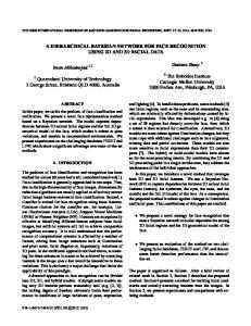
2. Bayesian Programming Probabilistic methodologies and techniques offer possible solutions to the incompleteness and uncertainty problems when programming a robot. The basic programming resources are probability distributions. In the context of probabilistic method, the Bayesian Programming (BP) approach was originally proposed as a tool for robotic programming (see [4]), but nowadays used in a wider scope of applications ([7,9] shows some examples). The Bayesian Programming formalism allows for using a unique notation and provides a structure to describe probabilistic knowledge and its use. The elements of a Bayesian Program are illustrated in Figure 1. A BP is divided in two parts: a description and a question. 2.1. Description The purpose of a description is to specify an effective method to compute a joint distribution on a set of relevant variables X1 , X2 , . . . , Xn , given a set of experimental data δ and a priori knowledge π. In the specification phase of the description, it is necessary to:
Guy Ramel et al. /
3
Pertinent Variables Decomposition ½ Specification(π) Parametric Forms Description Form Program Program Identification based on data(δ) Question
Figure 1. Structure of a Bayesian program.
• Define a set of relevant variables X1 , X2 , . . . , Xn , on which the joint distribution shall be defined • Decompose the joint distribution into simpler terms, using the conjunction rule. The conditional independence rule can allow further simplification, and such a simplified decomposition of the joint distribution is called decomposition • Define the forms for each term in the decomposition; i.e. each term is associated with either a parametric form, as a function, or to another Bayesian Program 2.2. Question Given a description P(X1 ∧ X2 ∧ ∧ Xn | δ ∧ π), a question is obtained by partitioning the variables X1 , X2 , . . . , Xn into three sets: Searched, Known and Unknown variables. A question is defined as the distribution P(Searched | Known ∧ δ ∧ π). In order to answer this question, the following general inference is used: P(Searched | Known ∧ δ ∧ π) = P U nknown P(Searched ∧ U nknown ∧ Known) P U nknown,Searched P(Searched ∧ U nknown ∧ Known)
(1)
3. Form Recognition with Bayesian Programming 3.1. Primitives In this work, we focus only on primitives features of low level. These ones are depicted in Figure 2. The primitives used are : vertical, horizontal, slash and backslash lines and four corners of different orientations. Several translated primitives of each type are added and used as Garbage Collector. Usage of garbage collector will be explained in the section 4. 3.2. Pertinent Variables The choice of the pertinent variables is a crucial point in defining a Bayesian program since it will be the backbone of the program and the quality of our detection will highly depend on it. These variables must not only be relevant for describing the features in terms of attributes and characteristics, but also, not be too numerous in order to keep the decision calculation time reasonable.
4
Guy Ramel et al. /
Figure 2. Set of primitives with “real” primitives (vertical, horizontal, slash and backslash line and the four corners) and several translated primitives of each type used as Garbage Collector.
Only one output variable is needed in our case. This is used to determine the type of the feature that have been recognized. This variable that is denoted by F eat. It is discrete and takes integer values over the range [0 . . . N ], where N corresponds to the number of different features that are searched in the image. In our case, all low-level features are recognised inside a window, which one scans the entire image. As shown in the figure 3, this window is divided into several square zones. In each of these zones, the ratio between the number of white pixels (contour pixels) called whitepix and the total number of pixels within a zone (called totpix) is employed for primitives detection. For each zone, this ratio is represented by a variable called Xi (i standing for a particular zone of a given feature) and is discrete over the interval IX = [0, 1]. This can be expressed as :
Xi =
whitepix totpix
(2)
These variables corresponds to the Known variable subset in our questioning inference . Therefore, the following joint distribution stands for our description of the problem: P (F eat ⊗ X1 ∧ . . . ∧ Xi | δ ∧ π)
(3)
3.3. Decomposition For this purpose, independence hypotheses need to be done in order to simplify the join decomposition. One can express this statement in the following way: P (X1 | F eat ∧ δ ∧ π)⊥ . . . ⊥P (Xi | F eat ∧ δ ∧ π). Under this hypothesis, using the product and marginalization rule, the decomposition becomes: P (F eat ∧ X1 ∧ . . . ∧ Xi | δ ∧ π) = P (F eat | δ ∧ π) × P (X1 | F eat ∧ δ ∧ π) × . . . . . . × P (Xi | F eat ∧ δ ∧ π) (4)
Guy Ramel et al. /
5
Figure 3. This figure depict how is divided the windows on several square zones. Each of these ones correspond to a variable. One see inside the window one feature (an upper-right corner)
3.4. Parametric forms Since no a priori information about the distribution of the features is available, one assume F eat to be uniformly distributed over [0 . . . N ] , i.e:
P (F eat = i) =
1 N
∀ i ∈ ℵ, [0 . . . N ]
One assume that these variables follows a Gaussian probability law where the mean and the standard deviation is dependent on the particular zone and the feature corresponding to the variable. P (Xi = x) = Gauss(µ(zone, F eat), σ(zone, F eat))
∀ i ∈