Simple Hybrid Model for Efficiency Optimization of Induction Motor ...

Hindawi Publishing Corporation Advances in Power Electronics Volume 2013, Article ID 371842, 8 pages http://dx.doi.org/10.1155/2013/371842

Research Article Simple Hybrid Model for Efficiency Optimization of Induction Motor Drives with Its Experimental Validation Branko Blanuša1 and Bojan Knezevic2 1 2

Faculty of Electrical Engineering, University of Banja Luka, Patre 5, 78000 Banja Luka, Bosnia and Herzegovina Faculty of Mechanical Engineering, University of Banja Luka, Bulevar Stepe Stepanovica 75, 78000 Banja Luka, Bosnia and Herzegovina

Correspondence should be addressed to Branko Blanuˇsa; [email protected] Received 28 December 2012; Revised 14 February 2013; Accepted 14 February 2013 Academic Editor: Jose Pomilio Copyright © 2013 B. Blanuˇsa and B. Knezevic. This is an open access article distributed under the Creative Commons Attribution License, which permits unrestricted use, distribution, and reproduction in any medium, provided the original work is properly cited. New hybrid model for efficiency optimization of induction motor drives (IMD) is presented in this paper. It combines two strategies for efficiency optimization: loss model control and search control. Search control technique is used in a steady state of drive and loss model during transient processes. As a result, power and energy losses are reduced, especially when load torque is significant less related to its rated value. Also, this hybrid method gives fast convergence to operating point of minimal power losses and shows negligible sensitivity to motor parameter changes regarding other published optimization strategies. This model is implemented in vector control induction motor drive. Simulations and experimental tests are performed. Results are presented in this paper.

1. Introduction Induction motor is a widely used electrical motor and a great energy consumer. The vast majority of induction motor drives are used for heating, ventilation, and air conditioning (HVAC). These applications require only low dynamic performance, and in most cases only voltage source inverter is inserted between grid and induction motor as cheapest solution. The classical way to control these drives is constant V/f ratio, and simple methods for efficiency optimization can be applied [1]. From the other side there are many applications where, like electrical vehicles, electric energy has to be consumed in the best possible way and use of induction motors. These applications require an energy optimized control strategy [2]. One interesting algorithm which can be applied in a drive controller is algorithm for efficiency optimization. In a conventional setting, the field excitation is kept constant at rated value throughout its entire load range. If machine is underloaded, this would result in overexcitation and unnecessary copper losses. Thus in cases where a motor drive has to operate in wider load range, the minimization of losses has great significance. It is known that efficiency

improvement of IMD can be implemented via motor flux level and this method has been proven to be particularly effective at light loads and in a steady state of drive. Also flux reduction at light loads gives less acoustic noise derived from both converter and machine. From the other side low flux makes motor more sensitive to load disturbances and degrades dynamic performances [3]. Drive loss model is used for optimal drive control in loss model control (LMC) [3–7]. These algorithms are fast because the optimal control is calculated directly from the loss model. But power loss modeling and calculation of the optimal control can be very complex. Often the loss model is not accurate enough. Search strategy methods have an important advantage compared to other strategies [8–11]. It is completely insensitive to parameter changes, while effects of the parameter variations caused by temperature and saturation are very expressed in two other strategies. The online efficiency optimization control on the basis of search, where the flux is decremented in steps until the measured input power settles down to the lowest value, is very attractive. Algorithm is applicable universally to any motor. Besides all good characteristics of search strategy methods, there is an outstanding

2

Advances in Power Electronics

problem in its use. For many applications flux convergence to its optimal value is too slowly. Also, flux is never reached its optimal value then in small steps oscillates around it. For electrical drives that work in periodic cycles, it is possible to calculate the optimal trajectory of magnetization flux, using optimal control theory, so that power losses in one working cycle are minimal [12]. These methods give good results if the working conditions do not change. Hybrid method combines good characteristics of two optimization strategies SC and LMC [3, 13–15]. It was enhanced attention as interesting solution for efficiency optimization of controlled electrical drives. During transient process LMC is used, so fast flux changes and good dynamic performances are kept. Search control is used for efficiency optimization in a steady state of drive. Loss model of IM in d-q rotational system and procedure for parameter identification in a loss model based on MoorePenrose pseudoinversion is given in Section 2. New hybrid model is presented in Section 3. Qualitative analyses of this method with simulation and experimental results are given in Section 4. At the end, obtained results are presented in Conclusion.

The process of energy conversion within motor drive converter and motor leads to the power losses in the motor windings and magnetic circuit as well as conduction and commutation losses in the inverter [6]. The losses in the motor consist of hysteresis losses and eddy current losses in a magnetic circuit (iron losses), losses in the stator and rotor windings (copper loss), and stray losses. In nominal operating conditions the iron losses are typically 2-3 times smaller than the copper losses, but at low loads, these losses are dominant. These losses consist of hysteresis and eddy current losses. Eddy current losses are proportional to the square of supply frequency, and hysteresis losses are proportional to supply frequency. Both components of iron losses are dependent of stator flux level, so next expression is suitable to represent these losses:

(3)

Based on the previous considerations, the losses in the induction motor drive, dependent on the magnetizing flux, can be expressed as follows: 2 2 𝑃𝛾 = (𝑅INV + 𝑅𝑠 ) 𝑖𝑠𝑑 + (𝑅INV + 𝑅𝑠 + 𝑅𝑟 ) 𝑖𝑠𝑞

(4)

2 2 + 𝑐eddy 𝜔𝑠2 𝜓𝑠𝑑 + 𝑐hys 𝜔𝑠 𝜓𝑠𝑑 .

Take into account expression for output power: 𝑃out = 𝑑𝜔𝜓𝑠𝑑 𝑖𝑠𝑞 ,

(5)

where 𝑃out is output power and 𝑑 is constant which depends on the characteristics of Park’s rotating transformation (in this case it is 1.5), and the relation 𝑃in = 𝑃𝛾 + 𝑃out

(6)

expression for input power can be written in the next form:

(2)

The total additional losses typically do not exceed 5% when the drive works with light loads. This case is the most important for the power loss minimization algorithms, so stray losses are not considered as a separate loss component. Losses in the drive converter consist of the losses in the rectifier and the conductive and switching losses in the inverter. The losses in the rectifier are independent of the

(7)

where 𝑎 = 𝑅𝑠 + 𝑅INV , 𝑏 = 𝑅𝑠 + 𝑅INV + 𝑅𝑟 , 𝑐1 = 𝑐eddy , 𝑐2 = 𝑐hys , and 𝑑 is positive constant. Two typical cases are differed: (1) linear dependence of magnetizing flux from the magnetizing current, (2) nonlinear dependence of magnetizing flux from the magnetizing current. In the algorithms for loss minimization, magnetizing flux is less than or equal to the nominal value, so it is used in the linear part of magnetization characteristics. Starting from the expressions (4) and taking into account expression (5), the power losses can be expressed as a function of 𝑖𝑠𝑑 , 𝑇em , and 𝜔𝑠 as follows: 𝑃𝛾 (𝑖𝑠𝑑 , 𝑇em , 𝜔𝑠 ) = (𝑎 + 𝑐1 𝐿2𝑚 𝜔𝑠2 + 𝑐2 𝐿2𝑚 𝜔𝑠 ) 𝑖𝑑2 +

2 𝑏𝑇em

2

(𝑑𝐿 𝑚 𝑖𝑠𝑑 )

(1)

where 𝑐eddy is eddy current and 𝑐hys is hysteresis loss coefficients. Copper losses are appeared as a result of the passing the electric current through the stator and rotor windings. These losses are proportional to the square of current through stator and rotor windings, and they are given by 2 . 𝑝𝛾Cu = 𝑅𝑠 𝑖𝑠2 + 𝑅𝑟 𝑖𝑠𝑞

2 2 + 𝑖𝑠𝑞 ). 𝑃INV = 𝑅INV 𝑖𝑠2 = 𝑅INV (𝑖𝑠𝑑

2 2 2 2 𝑃in = 𝑎𝑖𝑠𝑑 + 𝑏𝑖𝑠𝑞 + 𝑐1 𝜔𝑠2 𝜓𝑠𝑑 + 𝑐1 𝜔𝑠 𝜓𝑠𝑑 + 𝑑𝜔𝜓𝑠𝑑 𝑖𝑠𝑞 ,

2. Power Loss Modeling

2 2 2 𝜔𝑠 + 𝑐hys 𝜓𝑠𝑑 𝜔𝑠 , 𝑃𝛾Fe = 𝑐eddy 𝜓𝑠𝑑

magnetizing flux and not specifically taken into account. Only conductive losses in the inverter are dependent on the magnetizing flux, and these can be presented in the next form:

.

(8)

Slip angular speed can be defined as follows: 𝜔𝑠𝑙 = 𝜔𝑠 − 𝜔 ≈

𝑖𝑠𝑞 𝑇𝑟 𝑖𝑠𝑑

,

(9)

where 𝑇𝑟 is time rotor constant. Based on expression (8) power losses can be given as function of magnetizing current 𝑖𝑠𝑑 and operating conditions (𝜔, 𝑇em ): 2 𝑃𝛾 (𝑖𝑠𝑑 , 𝑇em , 𝜔) = (𝑎 + 𝑐1 𝐿2𝑚 𝜔2 + 𝑐2 𝐿2𝑚 𝜔) 𝑖𝑠𝑑

+

(2𝜔𝐿 𝑚 + 𝑐2 𝐿 𝑚 ) 𝑇em 𝑑𝑇𝑟

+

2 𝑇em 𝑐 𝑏 1 ( 2 + 12 ) 2 . 2 𝑑 𝐿 𝑚 𝑇𝑟 𝑖𝑠𝑑

(10)


3

2 Putting 𝑘1 = 𝑎 + 𝑐1 𝐿2𝑚 𝜔2 + 𝑐2 𝐿2𝑚 𝜔, 𝑘2 = (𝑇em /𝑑2 )(𝑏/𝐿2𝑚 + 2 𝑐1 /𝑇𝑟 ), and 𝑘3 = (2𝜔𝐿 𝑚 + 𝑐2 𝐿 𝑚 )𝑇em /𝑑𝑇𝑟 (10) can be written as follows:

𝑃𝛾 (𝑖𝑑 , 𝑇em , 𝜔) =

2 𝑘1 𝑖𝑠𝑑

∫

𝑘 + 22 + 𝑘3 . 𝑖𝑠𝑑

(11)

Parameter 𝑘3 is a function of 𝑇𝑟 which is time variant especially due to temperature changes. Time rotor constant is continuously updated in the algorithm for parameter identification, so the parameter 𝑘3 too. First and second derivations of 𝑃𝛾 in a function of 𝑖𝑠𝑑 are 𝜕𝑃𝛾 𝜕𝑖𝑑 𝜕 2 𝑃𝛾 𝜕2 𝑖𝑠𝑑

= 2𝑘1 + 6

= 2𝑘1 𝑖𝑠𝑑 − 2

𝑘2 , 4 𝑖𝑠𝑑

𝜕 2 𝑃𝛾 𝜕2 𝑖𝑠𝑑

> 0,

(12)

(13)

Based on the specified optimal value of 𝑑 component stator current vector and command of electromagnetic torque, 𝑞 component of the stator current is determined as follows: ∗ = 𝑖𝑠𝑞LMC

𝑇em . ∗ 𝑑𝐿 𝑚 𝑖𝑠𝑑LMC

(𝑛+1)𝑇

𝑛𝑇

𝑖𝑑2 (𝑡) 𝑑𝑡 + 𝑏 ∫

(𝑛+1)𝑇

+ 𝑐1 ∫

𝑛𝑇 (𝑛+1)𝑇

+ 𝑐2 ∫

𝑛𝑇

+ 𝑑∫

(𝑛+1)𝑇

(𝑛+1)𝑇

𝑛𝑇

𝑖𝑞2 (𝑡) 𝑑𝑡

[𝜓𝑑2 (𝑡) 𝜔𝑠2 (𝑡) 𝑑𝑡] [𝜓𝑑2 (𝑡) 𝜔𝑠 (𝑡) 𝑑𝑡] [𝜔 (𝑡) 𝑖𝑞 (𝑡) 𝜓𝑠𝑑 (𝑡) 𝑑𝑡] 󳨐⇒ (15)

Value 𝑖𝑠𝑑 max is chosen to be 𝐼𝑑𝑛 , and 𝑖𝑠𝑑 min is determined based on characteristics of drive and requirements for electromagnetic torque reserve. In this case 𝑖𝑠𝑑 min = 0.5𝐼𝑑𝑛 , where 𝐼𝑑𝑛 is nominal value of 𝑖𝑠𝑑 current. On the basis of expressions in (12), it can be concluded that in the steady state of drive and known operating conditions exists accurate value of 𝑖𝑠𝑑 which gives minimal losses as follows: 𝑘2 . 𝑘1

𝑛𝑇

𝑃in (𝑡) 𝑑𝑡 = 𝑎 ∫

𝑌𝑁 = 𝑎𝐴 𝑁 + 𝑏𝐵𝑁 + 𝑐1 𝐶𝑁1 + 𝑐2 𝐶𝑁2 + 𝑑𝐷𝑁.

for 𝑖𝑠𝑑 min ≤ 𝑖𝑠𝑑 ≤ 𝑖𝑠𝑑 max .

∗ = √4 𝑖𝑠𝑑LMC

(𝑛+1)𝑇

𝑛𝑇

𝑘2 , 3 𝑖𝑠𝑑

𝑘1 > 0, 𝑘2 > 0,

𝑊 = [𝑎 𝑏 𝑐1 𝑐2 𝑑]𝑇 , input signal and the input power are averaged in the period 𝑇 = 𝑄𝑇𝑆 :

(14)

2.1. Parameter Identification in a Loss Model. This procedure of parameter identification is a mainly based on the procedures described in [6, 7]. In order to determine the parameters in the model losses, 𝑎, 𝑏, 𝑐1 , and 𝑐2 , it is necessary to measure the input power and know the exact value of the output power. The exact value of the output power is needed to determine correct information of the losses in the drive and to avoid coupling between load pulsation and work of optimization controller. Also, the samples of the values that define input powers VDC , 𝑖DC (𝑃in = VDC 𝑖DC ) are available in the controller, and these values are used for protect and control functions (dynamic braking, the soft-start operation, PWM compensation, etc.). The proposed procedure of parameter identification is shown in Figure 1. The samples that exist in the expression (7) are memorized at each period. Usually the 𝑇𝑆 is 100–200 𝜇s. Due to high-frequency components that do not contribute to identification of the relevant parameters

Values 𝐴 𝑁, 𝐵𝑁, 𝐶𝑁1 , 𝐶𝑁2 , and 𝐷𝑁, 𝑁 = 1, . . . , 𝑀 successively form the columns 𝑃(:, 1), 𝑃(:, 2), 𝑃(:, 3), 𝑃(:, 4), and 𝑃(:, 5) of matrix 𝑃𝑀×5 . Vector 𝑌 is formed from 𝑀 averaged values of input power 𝑌𝑁, 𝑁 = 1, . . . , 𝑀. Vector 𝑊𝑔 is calculated by applying Moore-Penrose pseudoinversion (Figure 1) as follows: 𝑇

−1

𝑊𝑔 = [𝑎𝑔 𝑏𝑔 𝑐𝑔1 𝑐𝑔2 𝑑𝑔 ] = (𝑃𝑇 𝑃) 𝑃𝑌.

(16)

That is 𝑊𝑔 is approximate solution of the matrix equations 𝑃𝑊 = 𝑌, which gives a minimum value ‖𝑃𝑊 − 𝑌‖ or minimum mean-square error. The choice of 𝑄 is of great importance for the process of parameters identification (see (15)) because the input power fluctuations should be sufficient in the period 𝑇 = 𝑄𝑇𝑆 . Otherwise 𝑃𝑇 𝑃 matrix will be singular or aspire singularity, that is, det (𝑃𝑇 𝑃) will be close to 0. The process of determining the parameters in the loss model is repeated during the operation of electric drive.

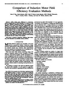
3. Hybrid Model for Efficiency Optimization Electrical drive with block for efficiency optimization is shown in Figure 2. Electric drive is supplied from the primary power network 3×380 V. This voltage is rectified, and the voltage and current in DC link are measured. The drive inverter is current regulated (CR) voltage three-phase inverter. Reference and measured 𝑑 and 𝑞 components of stator current are kept in the current controllers. These controllers are realized in rotational 𝑑, 𝑞 coordinate system as a linear PI controller. Outputs of controller are 𝑑 and 𝑞 component of stator voltage. These voltages are transformed (B-transformation) in threephase reference voltages V𝑎∗ , V𝑏∗ , and V𝑐∗ . These voltages are scaled and lead to PWM modulator, where control signals of inverter switches are generated. This drive works as speed controlled drive. Speed reference and measured speed are led into speed controller. Speed controller is realized as PI controller in incremental form, with proportional coefficient in a feedback local branch. The output of speed controller is reference value of electromagnetic torque. Reference value of stator current 𝑑 component is determined in a block for efficiency optimization and 𝑞 component of stator current

4


2 𝑖𝑠𝑞

2 2 𝜓𝑠𝑑 𝜔𝑠

2 𝜓𝑠𝑑 𝜔𝑠

𝑢1

𝑗=𝑄 𝑢

∑

𝑗=1

𝑢2

𝑗=𝑄 𝑢

∑

𝑗=1

𝑢3

𝑗=𝑄 𝑢

∑

𝑗=1

𝑢4

𝑗=𝑄 𝑢

∑

𝑗=1

1 (𝑛𝑇 +

𝑗)𝜏

𝐴 𝑛 𝑃(:, 1) = [𝐴 𝑛0 · · · 𝐴 𝑛0+𝑀 ]𝑇

2 (𝑛𝑇 +

𝑗)𝜏

𝐵𝑛

3 (𝑛𝑇 +

𝑗)𝜏

𝐶𝑛1 𝑃(:, 3) = [𝐶𝑛0 · · · 𝐶𝑛0+𝑀 ]𝑇

𝑄

𝑄

𝑄

4 (𝑛𝑇 +

𝑗)𝜏

𝑄

𝑃(:, 2) =

[𝐵𝑛0 · · · 𝐵𝑛0+𝑀 ]𝑇

𝑃(:, 1)

𝑃(:, 2)

𝑃(:, 3)

𝐶𝑛2 𝑃(:, 3) = 𝑃(:, 4) [𝐶𝑛20 · · · 𝐶𝑛20+𝑀 ]𝑇

𝑃(𝑀×5) MATRICA

2 𝑖𝑠𝑑

∣det(𝑃𝑇 𝑃)∣0.25 𝑃 𝑇

[𝑎𝑔 𝑏𝑔 𝑐1𝑔 𝑐2𝑔 𝑑𝑔 ] =

𝑊𝑔 = [𝑎𝑔 𝑏𝑔 𝑐1𝑔 𝑐2𝑔 𝑑𝑔 ]

𝑇

(𝑃𝑇 𝑃)−1 𝑃𝑇 𝑌 𝑌

𝑖𝑠𝑞 𝜓𝑠𝑑 𝜔

𝑃in(DC)

𝑢5

𝑗=𝑄 𝑢

∑

𝑗=1

𝑢6

𝑗=𝑄 𝑢

∑

𝑗=1

5 (𝑛𝑇 +

𝑗)𝜏

𝐷𝑛 𝑃(:, 4) = [𝐷𝑛0 . . . 𝐷𝑛0+𝑀 ]𝑇

5 (𝑛𝑇 +

𝑗)𝜏

𝑌𝑛

𝑄

𝑄

𝑃(:, 5)

𝑌= [𝑌𝑛0 · · · 𝑌𝑛0+𝑀 ]𝑇

Figure 1: A method for determining the parameters 𝑎, 𝑏, 𝑐1 , 𝑐2 and, 𝑑 from the input signal.

vector on the basis of 𝑑 stator current vector component and electromagnetic torque reference (see (14)). Position of rotor flux vector is determined in indirect vector control block (IVC). Hybrid model for efficiency optimization consists from 3 blocks, LMC, SC, and steady state control (SSC) block. LMC is used during transient states caused of external speed ∗ ∗ , 𝑖𝑠𝑞LMC ) is or torque demand [3]. Optimal control (𝑖𝑠𝑑LMC calculated directly from loss model for a given operational conditions what obtains power loss optimization and good dynamic performances. SC is used in a steady state for a constant output power. On the basis of speed reference and measured speed, SSC block defines its output and controls switches (Figure 2). If transient states is detected, LMC is active, and its outputs are forwarded to indirect vector control (IVC) block and current regulators. When steady state is detected in SSC block, last value of magnetizing current during transient state is used as starting point for search algorithm.

3.1. Loss Model Controller. Optimal control calculation in LMC for a given operational conditions is described in Section 2. Expressions for 𝑑 and 𝑞 component of stator current are defined by (8) and (10). This method is sensitive to parameter changes due to temperature changes and magnetic circuit saturation, what consequently leads to error in a current references calculation. So, algorithm for parameter identification is always active, and parameters in the loss model are continuously updated (Figure 2).

3.2. Search Controller. Search algorithm is used in steady state, which is detected in the SSC block. Error that exists between the current reference 𝑖𝑑 that is generated in the LMC model and in the search model appears as a consequence of inverter and stray losses which are not included in the model. The applied search algorithm is simple. Since the current 𝑖𝑠𝑑 is very close to the value which gives minimal losses, small step of magnetization current Δ𝑖𝑠𝑑 = 0.01𝐼𝑑𝑛 is chosen. For two successive values of the 𝑖𝑠𝑑 current, power losses are determined. Sign of Δ𝑖𝑠𝑑 is maintained if power losses are reduced. Otherwise, the sign of Δ𝑖𝑠𝑑 is opposite in the next step: 𝑖𝑠𝑑 (𝑛) = 𝑖𝑠𝑑 (𝑛 − 1) − sgn (Δ𝑃𝛾 (𝑛 − 1)) Δ𝑖𝑠𝑑 .

(17)

When the two values of magnetization current 𝑖𝑠𝑑1 and 𝑖𝑠𝑑2 were found, so the sign of power loss is changed between these values, and new reference of 𝑖𝑠𝑑 current is specified as: ∗ 𝑖𝑠𝑑SC =

𝑖𝑠𝑑1 + 𝑖𝑠𝑑2 . 2

(18)

In this way, there are no oscillations of 𝑖𝑠𝑑 current, air gap flux, and electromagnetic torque, which are characteristics of the search algorithm.

4. Simulation and Experimental Results 4.1. Simulation Results. Hybrid method for efficiency optimization of IMD has been studied through computer simulation in MATLAB-Simulink. Speed reference and load torque are shown in Figure 3. The steep change of load torque appears with the aim


𝑃out

5 ∗ 𝑖𝑠𝑞𝑆𝐶

𝑃in ∗ = 𝜔 ∗ 𝑇em

𝑆𝐶

∗ 𝑖𝑠𝑑𝑆𝐶 ∗ 𝑖𝑠𝑑

1/𝑧 𝜔∗

Steady state control

𝜔

𝐿𝑀𝐶 𝑎 𝑏 𝑐1 𝑐2 𝑑

𝜔∗ + Δ𝜔 Speed reference − 𝜔

PI speed controller

SW3

𝑣𝑑∗ 𝑣𝑞∗ 𝜃𝑠

Power supply 3 × 230 V 50 Hz

2Φ

𝐵−1

∗ 𝑖𝑠𝑞

∗ 𝑖𝑠𝑞𝐿𝑀𝐶

∗ 𝑇em

𝑇em Torque estimator

𝜃𝑠∗

𝐼𝑉𝐶

1

2

3

𝑖𝑠𝑑 𝑖𝑠𝑞 𝜔 𝜔𝑠 𝜓𝑠𝑑 𝑃in

𝑣𝑎∗ ∗ 3Φ 𝑣𝑏 𝑣𝑐∗

3Φ

𝐵

𝑖𝑎 𝑖𝑏

CRPWM VSI

Rectifier 𝑖DC 𝑣DC

𝑣𝑞∗

𝑞 PI current controller

SW2

Loss model parameter identification

𝜃𝑠 1 2 3

SW1

∗ 𝑖𝑠𝑑𝐿𝑀𝐶

𝑣𝑑∗

𝑑 PI current controller

𝑣𝑎 𝑣𝑏 𝑣𝑐

𝑖𝑠𝑑 2Φ 𝑖 𝑠𝑞 𝑖𝑐

Incremental encoder interface

𝐴𝑀 Encoder

𝜔

Power calculation 𝑃in

Figure 2: Overall proposed block diagram of efficiency optimization controller in IMD.

of testing the drive behavior in the dynamic mode and its robustness for a sudden load perturbations. Graphs of magnetization current (𝑖𝑠𝑑 ) and active component (𝑖𝑠𝑞 ) of stator current vector for a given operating conditions and applied hybrid method are shown in Figure 4. Graphs of power loss for nominal flux and hybrid method are given in Figure 5. It is obvious that the use of hybrid methods gives significantly less power losses than when the flux is maintained at nominal value for a light load of drive.

1 0.8 Speed reference p.u.

0.6 0.4

Load torque p.u.

4.2. Experimental Results. The experimental tests have been performed on the setup which consists of the following: (i) induction motor (3 phases, Δ380 V/𝑌220 V, 3.7/2.12 A, cos 𝜙 = 0.71, 1410 r/min, 50 Hz), (ii) incremental encoder connected with the motor shaft, (iii) three-phase drive converter (DC/AC converter and DC link), (iv) PC and dSPACE1102 controller board with TMS320C31 floating point processor and peripherals, (v) interface between controller board and drive converter.

0.2 0

0

2

4

6 Time (s)

8

10

12

Figure 3: Speed reference and load torque [p.u.].

Parameters of used induction motor are given in the appendix of the paper.

6

Advances in Power Electronics 200

1.4

Power losses (10 W/div)

𝑖𝑑 and 𝑖𝑞 stator currents

1.2 1 0.8 0.6

150

100

50

0.4 0

0.2 0

0

2

4

6

8

10

12

Time (0.5 s/div)

0

2

4

6 Time (s)

8

10

12

Figure 6: Power losses for nominal magnetization flux and operational conditions shown in Figure 3.

Current 𝑖𝑑 p.u. Current 𝑖𝑞 p.u.

Figure 4: Graphs of 𝑑 and 𝑞 component of stator current for a given operating conditions. Power losses (10 W/div)

160 140 120 Power losses (W)

200

150

100

50

100 Nominal flux

80 60

0

2

4

6

8

10

12

Time (0.5 s/div)

Hybrid method

40

Figure 7: Power losses when the hybrid method is applied and operational conditions shown in Figure 3.

20 0

0

0

2

4

6 Time (s)

8

10

12

Figure 5: Graph of power loss for nominal flux and applied hybrid method.

The algorithm observed in this paper used the MATLABSimulink software, dSPACE real-time interface, and C language. Handling real-time applications is done in ControlDesk. All experimental tests and simulations have been done in the same operating conditions of the drive, and some comparisons between algorithms for efficiency optimization are made through the experimental tests. Graphs of power losses for nominal flux and when the hybrid method is applied are shown in Figures 6 and 7, respectively. Graphs of magnetization current for a given operational conditions are shown in Figure 8, and speed response is shown in Figure 9.

Based on graph in Figure 6, it can be concluded that the speed drop for a step change of load is small and speed response is strictly aperiodic.

5. Conclusion Algorithms for efficiency optimization of induction motor drive are briefly described. Detailed theoretical analysis of power losses in induction motor is presented. Algorithm for parameter identification in the loss model based on MoorePenrose pseudoinversion is presented. Also, hybrid algorithm for efficiency optimization has been applied. According to the theoretical analysis, performed simulations, and experimental tests we have arrived to the following conclusions. If load torque has a value close to nominal or higher, magnetizing flux is also nominal regardless of whether an algorithm for efficiency optimization is applied or not.


7 0.75 kW (nominal mechanical power)

2.5

cos 𝜙 = 0, 71 (power factor)

𝑖𝑞

1410 r/min (nominal mechanical speed)

Currents 𝑖𝑑 , 𝑖𝑞 (0.1 A/div)

2

𝑅𝑠 = 10.4 Ω (stator resistance)

𝑖𝑑

1.5

𝑅𝑟 = 11.6 Ω (rotor resistance) 𝐿 𝛾𝑠 = 22 mH (stator leakage inductance) 𝐿 𝛾𝑟 = 22 mH (stator leakage inductance)

1

𝐿 𝑚𝑛 = 0, 557 H (magnetization inductance) 𝐽𝑚 = 0, 0072 kgm2 (inertia moment)

0.5

𝐼𝑑𝑛 = 1.501 A (nominal value of 𝑖𝑠𝑑 current) 0

0

2

4

6

8

10

Time (0.5 s/div)

Figure 8: Magnetization current 𝑖𝑑 and active current when the hybrid method is applied and operational conditions shown in Figure 3. 160

120

Speed (rad/s)

𝐼𝑞𝑛 = 2.093 A (nominal value of 𝑖𝑠𝑞 current).

12

80

40

Nomenclature 𝑅𝑠 , 𝑅𝑟 : 𝐿 𝑠, 𝐿 𝑟: 𝐿 𝑚: 𝜎: 𝐿󸀠𝑠 : 𝑃: 𝜗𝑠 , 𝜔𝑠 : 𝜗, 𝜔: 𝜔𝑠 : 𝑇em : 𝜓𝑠𝑑 : 𝑖𝑠𝑑 , 𝑖𝑠𝑞 :

Resistance of stator and rotor winding Self-inductance of stator and rotor Magnetizing inductance Leakage factor Stator transient inductance Number of pole pairs Rotor flux angle and angular speed Rotor angle and angular speed slip speed Elektromagnetic torque Magnetizing flux 𝑑 and 𝑞 components of stator current vector.

References 0

0

2

4

6

8

10

12

Time (0.5 s/div)

Figure 9: Speed response when the hybrid method is applied and operational conditions shown in Figure 3.

For a light load, hybrid method for efficiency optimization gives significant power loss reduction (Figures 5, 6, and 7). There is no oscillation of magnetization flux which is characteristic of the search algorithms (Figures 4 and 8). Also, this hybrid method shows good dynamic performances and no sensitivity to parameter changes (Figure 9). Implementation of presented algorithm is simple, and it can be universally applied to any electrical motor. Changes are only related to different models of power losses.

Appendix Parameters of used induction motor 3 phase Δ220/Y380 V (supply voltage) 3,7/2,12 A (nominal stator current)

[1] F. Abrahamsen, F. Blaabjerg, J. K. Pedersen, P. Z. Grabowski, and P. Thgersen, “On the energy optimized control of standard and high-efficiency induction motors in CT and HVAC applications,” IEEE Transactions on Industry Applications, vol. 34, no. 4, pp. 822–831, 1998. [2] M. Chis, S. Jayaram, and K. Rajashekara, “Neural networkbased efficiency optimization of EV drive,” in Proceedings of the Canadian Conference on Electrical and Computer Engineering (CCECE ’97), pp. 454–457, May 1997. [3] E. S. Sergaki and G. S. Stavrakakis, “Online search based fuzzy optimum efficiency operation in steady and transient states for DC and AC vector controlled motors,” in Proceedings of the International Conference on Electrical Machines (ICEM ’08), Vilamoura, Portugal, September 2008. [4] F. Abrahamsen, J. K. Pedersen, and F. Blaabjerg, “State-of-Art of optimal efficiency control of low cost induction motor drives,” in Proceedings of Conference on Fuzzy Systems (PESC ’96), pp. 920–924, 1996. [5] M. N. Uddin and S. W. Nam, “Development of a nonlinear and model-based online loss minimization control of an IM drive,” IEEE Transactions on Energy Conversion, vol. 23, no. 4, pp. 1015– 1024, 2008. [6] B. Blanusa, P. Matić, Z. Ivanovic, and S. N. Vukosavic, “An improved loss model based algorithm for efficiency optimization of the induction motor drive,” Electronics, vol. 10, no. 1, pp. 49–52, 2006.

8 [7] S. N. Vukosavic and E. Levi, “Robust DSP-based efficiency optimization of a variable speed induction motor drive,” IEEE Transactions on Industrial Electronics, vol. 50, no. 3, pp. 560– 570, 2003. [8] G. C. D. Sousa, B. K. Bose, and J. G. Cleland, “Fuzzy logic based on-line efficiency optimization control of an indirect vector-controlled induction motor drive,” IEEE Transactions on Industrial Electronics, vol. 42, no. 2, pp. 192–198, 1995. [9] D. de Almeida Souza, W. C. P. de Aragao Filho, and G. C. D. Sousa, “Adaptive fuzzy controller for efficiency optimization of induction motors,” IEEE Transactions on Industrial Electronics, vol. 54, no. 4, pp. 2157–2164, 2007. [10] S. Ghozzi, K. Jelassi, and X. Roboam, “Energy optimization of induction motor drives,” in Proceedings of the IEEE International Conference on Industrial Technology (ICIT ’04), pp. 602–610, December 2004. [11] Z. Liwei, L. Jun, W. Xuhui, and T. Q. Zheng, “Systematic design of fuzzy logic based hybrid on-line minimum input power search control strategy for efficiency optimization of IM,” in Proceedings of the CES/IEEE 5th International Power Electronics and Motion Control Conference (IPEMC ’06), pp. 1012–1016, August 2006. [12] B. Blanusa and S. N. Vukosavic, “Efficiency optimized control for closed-cycle operations of high performance induction motor drive,” Journal of Electrical Engineering, vol. 8, pp. 81–88, 2008. [13] C. Chakraborty and Y. Hori, “Fast efficiency optimization techniques for the indirect vector-controlled induction motor drives,” IEEE Transactions on Industry Applications, vol. 39, no. 4, pp. 1070–1076, 2003. [14] B. Blanuˇsa, P. Matić, and B. Dokić, “New hybrid model for efficiency optimization of induction motor drives,” in Proceedings of 52nd International Symposium ELMAR-2010, pp. 313–317, 2010. [15] P. Was, Electrical Machines and Drives, Oxford University Press, 1992.


International Journal of

Rotating Machinery

Engineering Journal of

Hindawi Publishing Corporation http://www.hindawi.com

Volume 2014

The Scientific World Journal Hindawi Publishing Corporation http://www.hindawi.com

Volume 2014


Distributed Sensor Networks

Journal of

Sensors Hindawi Publishing Corporation http://www.hindawi.com

Volume 2014


Volume 2014


Volume 2014

Journal of

Control Science and Engineering

Advances in

Civil Engineering Hindawi Publishing Corporation http://www.hindawi.com


Volume 2014

Volume 2014

Submit your manuscripts at http://www.hindawi.com Journal of

Journal of

Electrical and Computer Engineering

Robotics Hindawi Publishing Corporation http://www.hindawi.com


Volume 2014

Volume 2014

VLSI Design Advances in OptoElectronics


Navigation and Observation Hindawi Publishing Corporation http://www.hindawi.com

Volume 2014



Chemical Engineering Hindawi Publishing Corporation http://www.hindawi.com

Volume 2014

Volume 2014

Active and Passive Electronic Components

Antennas and Propagation Hindawi Publishing Corporation http://www.hindawi.com

Aerospace Engineering


Volume 2014


Volume 2014

Volume 2014




Modelling & Simulation in Engineering

Volume 2014


Volume 2014

Shock and Vibration Hindawi Publishing Corporation http://www.hindawi.com

Volume 2014

Advances in

Acoustics and Vibration Hindawi Publishing Corporation http://www.hindawi.com

Volume 2014