179
Simple Models of Zero-Net Mass-Flux Jets for Flow Control Simulations Reni Raju Dynaflow Inc., Jessup, MD – 20794 Ehsan Aram and Rajat Mittal1 Department of Mechanical Engineering, Johns Hopkins University, Baltimore, MD – 21218 Louis Cattafesta Department of Mechanical and Aerospace Engineering, University of Florida, Gainesville, FL – 32611 Abstract Although computational fluid dynamics is well suited for modeling the dynamics of zeronet mass-flux (ZNMF) actuators, the computational costs associated with large-scale flow control simulations necessitate the use of simple models for these devices. A new model based on only the slot of ZNMF jets in grazing flows is proposed. A study of the dimensionless parameters governing the ZNMF jet in grazing flow is conducted, and the performance of the model is assessed in terms of the vortex dynamics and the mean integral quantities that define characteristics of the ZNMF jet. A comparison with full cavity simulations as well as the often-used sinusoidal, plug-flow model indicates that the new model provides a good prediction of the jet outflow. In addition, the fidelity of the model has also been explored for a canonical separated flow. Results show that the model is able to predict the effect of the jet on the separation bubble much more accurately than the conventional plug-flow model.
1. INTRODUCTION Zero-net mass-flux (ZNMF) actuators or “synthetic jets” have potential applications in the areas of mixing enhancement [1,2], heat transfer [3-5], mass transfer [6], jet vectoring [7], and active flow control of separation [8-10] and turbulence [11]. The dynamics and performance of these devices depend on several geometrical, structural and flow parameters [12-14]. When compared to the global domain, such as an airfoil in which the actuator is imbedded, the scales of the actuator are typically 10-2 – 10-4 times smaller in size. Due to the range of scales involved, inclusion of a high-fidelity model of a ZNMF actuator within a macro-scale computational flow model is an expensive, if not prohibitive, proposition. The desire to compute the flow physics associated with the ZNMF jet control makes it a practical necessity that simple yet accurate models of these devices be devised and employed in such computations. In many past simulations, these actuators have been represented via simplified models in one form or another. Kral et al. [15] modeled the actuator via temporal sinusoidal, surface boundary conditions for velocity and pressure without the slot and cavity. For a ZNMF jet exhausting in a quiescent external flow, they noted that the “top-hat” shaped jet velocity profile provided the closest match to the experiments. Rizzetta et al. [16] used the recorded flow field from a simulation of the isolated jet at the exit of a 2D periodic jet as a boundary condition to an external flow field. On the other hand, Lockerby et al. [17] used a theoretical approach based on classic thin plate theory to model the diaphragm deflection, while the slot is modeled based on unsteady pipe-flow theory. A reduced-order model approximating 2D or 3D synthetic jets via quasi-1D Euler equations was presented by Yamaleev et al. [18,19]. Filz et al. [20] modeled 2D directed synthetic jets using lumped deterministic source terms (LDST) trained by a neural network. Rathnasingham and Breuer [21] presented a semi-empirical model of ZNMF actuators using a system of coupled nonlinear state equations describing the structural and fluid characteristics of the device. An analytical lumped element model (LEM) of a piezoelectric-driven 1Corresponding
author,
[email protected]
Volume 1 · Number 3 · 2009
180
Simple Models of Zero-Net Mass-Flux Jets for Flow Control Simulations
and an electrodynamic synthetic jet was developed by Gallas et al. [12] and Agashe et al. [22], respectively. The LEM represented the individual components of the synthetic jet as elements of an equivalent electric circuit using conjugate power variables. Sharma [23] used an alternate model for LEM. More recently, Tang et al. [24] compared the performance of the Dynamic Incompressible Flow model (DI model), Static Compressible Flow Model (SC model) and LEM in predicting the instantaneous space-averaged velocity at the orifice exit. Low-order modeling of two-dimensional synthetic jets via Proper Orthogonal Decomposition (POD) was carried out by Rediniotis et al. [25] The dynamical model based on Galerkin projection was derived from the flow for specific Reynolds and Stokes numbers. Kihwan et al. [26] developed a dynamical model based on system identification to identify the interaction of synthetic jets with a laminar boundary layer with potential application to feedback control. The temporal sinusoidal profile used by Kral et al. [15] is perhaps the simplest model of the jet and is referred to as the “modified boundary condition” (MBC) model in the current study, which defines the wall normal velocity as v( x, y = 0, t ) = Vo f ( x )sin(ωt )
(1)
Three different spatial distribution functions were considered 1 f ( x ) = sin(π x / d ) sin 2 (π x / d )
(2)
Of these, Kral et al. found the f(x)=1 or or “plug-flow” profile provides the best agreement with experiments. A modified boundary condition for pressure as a function of wall-normal velocity was also used. Such a simple representation eliminates the need to simulate the cavity and the slot. A similar approach has also been adopted in some later studies by Rampunggoon [27] that considered a family of jet profiles. The parameters studied included the skewness of the profile, centerline velocity and momentum coefficient. Recent work by Ravi [28] considered several candidate profiles for jets in grazing flow, including a steady blowing profile, unsteady sinusoidal profiles and profiles based on numerical calculations. For the sinusoidal profile, both plug-flow and triangular spatial distributions were considered. Numerical profiles extracted from baseline calculations were prescribed as boundary conditions for only the crossstream velocity in one case and for both velocity components in another. As expected, the numerical profiles provided better accuracy in comparison to the simple boundary conditions. This approach of using the recorded flow field at the exit of a 2D periodic jet as a boundary condition to an external flow field was also used earlier by Rizzetta et al. [16]. However, such prescriptions are “postdictive” in that they first require simulations with a full cavity from which the boundary conditions can be recorded, and are therefore not practical as predictive actuator models. This paper explores the issues of local actuator modeling in numerical simulations of flow control. While previous studies have focused on the fidelity of simple “surface” boundary conditions, in the current study we investigate the impact of including the slot geometry along with simplified boundary conditions. Based on numerical simulations we propose a new model for ZNMF jets in grazing flows. The model is based on retaining the minimal geometrical features of the actuator and on a phenomenological flow prescription. The key features of the model are that it is fully predictive and offers significant simplifications in the inclusion of ZNMF jets in large-scale flow simulations. The proposed model is compared with the full cavity simulations and the MBC model of Kral et al. [15] in attached grazing flows to demonstrate its capabilities and limits. Subsequently, the effectiveness of the proposed model is also examined for a canonical separated boundary layer flow. 2. SLOT-ONLY ZNMF ACTUATOR MODEL Neglecting the flow physics associated with the jet slot is one of the primary reasons for the shortcomings of the modified boundary condition models. Our previous studies [29] show that the flow in the slot tends to separate at the top and bottom lips during the expulsion and ingestion phases. Figure 1 shows vorticity contours and vectors of such a typical case at different phases in the cycle of operation of a ZNMF jet in a quiescent condition. As seen, the formation of secondary vortices near the exit tends International Journal of Flow Control
Reni Raju, Ehsan Aram, Rajat Mittal and Louis Cattafesta
181
to significantly alter the flow field. Thus, the working hypothesis for the current model is that the inclusion of just the slot with appropriate boundary conditions at the slot entrance should significantly improve the fidelity of the actuator model. This hypothesis is supported by past studies [30,31] that have shown that the shape of the cavity has little effect on the flow emanating from the jet provided that the incompressible flow assumption inside the actuator cavity is valid. The approach used for the current study explores the significance of the slot via simplified boundary conditions and hence effectively reduces the computational complexity. An attempt is thus made to replicate the flow physics inside the slot to further improve the fidelity of the model.
φ ~90°
φ ~0°
(b)
(a)
φ ~180°
(c)
φ ~270°
(d)
Figure 1. Instantaneous spanwise vorticity contours and velocity vectors at (a) φ ∼ 0°, (b) φ ∼ 90° (peak expulsion), (c) φ ∼ 180° and (d) φ ∼ 270° (peak ingestion) for a typical ZNMF actuator in a quiescent medium to illustrate the complexity of the flow in the slot.
Consider the flow inside the 2D slot of a typical ZNMF actuator as seen in Figure 2(a). The area change from the cavity to the slot causes the flow to turn near the bottom lip of the slot, and the flow pattern during expulsion is similar to the one caused by a sink present somewhere along the slot center during the expulsion phase. The validity of this assumption is apparent by observing the velocity vectors at φ = 90° in Figure 1(b), inset. Note that the expulsion stroke is defined as 0° ≤ φ 180° and ingestion stroke as 180° ≤ φ 360°. Hence the flow enters the slot radially at any given time during expulsion and, in terms of its Cartesian components, will have two components of velocity, lateral u and vertical v. As seen in Figure 2(a), at the entrance to the slot (i.e., at x = ±d/2, y = H) the u velocity will be significant, while near the slot center the v velocity will dominate. Thus an approximation of this flow pattern prescribes a corresponding boundary condition profile for the u velocity at the slot boundary, y=H, which varies linearly in the x-direction from a maximum positive value near the left wall to a minimum negative value near the right wall of the form (–xU0 sin(ωt)/d/2 for –d/2 < x < d/2 and 0 at x = ±d/2. 2.1 Model Comparison Based on the above arguments, three separate flow configurations (or “models”) have been chosen for comparison. These include the full-cavity (FC), the slot-only (SO), and modified boundary condition (MBC) configurations. As the name suggests, the FC model consists of full-cavity simulations and is Volume 1 · Number 3 · 2009
182
Simple Models of Zero-Net Mass-Flux Jets for Flow Control Simulations
(a)
(b)
(c)
(d)
Figure 2. Schematic showing (a) the typical flow pattern seen in a ZNMF jet slot for a full cavity (FC) configuration, (b) the modified boundary condition (MBC), and variants of proposed slot-only (SO) models in (c) SO-1 and (d) SO-2.
considered a complete and accurate representation of a 2D ZNMF jet, as seen in Figure 2(a). The driver displacement is represented as an oscillatory boundary condition at the bottom of the cavity, and this has been found to be a fairly accurate representation for an incompressible flow assumption when compared with experimental results [30]. Figure 2(b) shows the MBC configuration, which, as mentioned earlier, consists of prescribing only the vertical component of the velocity over the exit plane of the jet. Finally, the proposed SO model is based on the configuration shown in Figure 2(c-d) which includes the slot of the actuator but not the cavity. Based on our observations, we expect that the slotonly model, with an appropriate boundary condition prescription at the entrance to the slot, will be able to replicate the jet characteristics very accurately, albeit without the computational expense associated with including the full cavity. Thus, the SO models can be considered intermediate to the FC and MBC models. The key then is to determine the appropriate boundary conditions that can be applied at the slot entrance and to assess the fidelity of this model versus the other models. The dimensionless parameters of significance for a ZNMF jet issuing into a grazing laminar — boundary layer are the Stokes number S = ω d 2 / υ , jet Reynolds number, ReJ = VJd/υ, velocity ratio, — U∞/ VJ and boundary-layer thickness to jet width ratio, δ/d. Here ω is the angular frequency, while T /2 d 2 1 VJ = v( x, t ) dx dt is the spatially and temporally averaged jet expulsion velocity at the jet T d ∫ ∫ 0
0
exit, and υ is the kinematic viscosity. Alternatively the Stokes number or jet Reynolds number can also — be replaced by the Strouhal number, St = ωd/ VJ = S2/ReJ. The boundary-layer thickness, δ, is defined as the distance from the wall where u/U∞ = 0.99 . Two variants of the slot-only models are considered. For the first, called the SO-1 model, represented in Figure 2(c), only the sinusoidal v velocity (vertical velocity) is prescribed at the bottom of the slot at its junction with the cavity, while for the second, the SO-2 model, as seen in Figure 2(d), boundary conditions for both the u & v velocities during expulsion have been used. As described above, the u velocity is prescribed as a linearly varying sinusoidal profile that satisfies no-slip condition at the slot edges. The linear variation in the horizontal velocity is based on the sink-like flow behavior at the slot inlet wherein this velocity is zero at the slot center and increases to a maximum value near the slot walls. It should also be noted that the expulsion and ingestion portions of the cycle produce very different flow at the slot inlet and exit, so we assume different velocity prescriptions for these two phases. Table 1 lists the boundary conditions used for the different configurations during both expulsion and ingestion phases with the corresponding location. With the exception of FC simulation where u = 0 at the bottom wall, outflow is ensured by providing Neumann boundary conditions for the horizontal component — during the ingestion phase. Note that in the table below, mass conservation implies that V0 = (π/2) VJ. While the vertical velocity V0 is determined from the mass-flux, the horizontal velocity amplitude U0 International Journal of Flow Control
Reni Raju, Ehsan Aram, Rajat Mittal and Louis Cattafesta
183
at the slot inlet needs to be prescribed. Noting that for a line sink, axisymmetry would produce the same radial velocity at all azimuth around the point, we choose U0 = V0 for all the cases. With this prescription, the slot model is fully closed in that it does not have any undetermined parameters. Table 1. Boundary conditions used for different configurations/models considered in the current study.
Model
Expulsion
y d location w.r.t. FC
Ingestion
v( x, t )
u( x , t )
v( x, t )
∂u ( x, t ) ∂y
0
V0 d sin(ωt ) W
-
FC
0
V0 d sin(ωt ) W
MBC SO-1
h+H
V0 sin(ωt )
H
V0 sin(ωt )
0 0
V0 sin(ωt ) V0 sin(ωt )
0 0
V0 sin(ωt )
0
−x U 0 sin(ωt ) d 2
SO-2
V0 sin(ωt )
H
for − d < x < d 2 2 0 at x = ± d 2
The objective now is to determine the relative fidelity of the three simple models for a range of operational parameters. Note that the FC configuration is considered exact and all other models are compared to this to assess fidelity. The model assessment has been performed over a wide range of operational parameters. Dimensional analysis [29] indicates that the jet characteristics depend on the — parameters as St, U∞/ Vj, δ/d, ReJ and Table 2 lists the cases studied. Hence for the current study, three different simulation sets were considered for each of these parameters while keeping everything else the same. Table 2. Parameters used for ZNMF model assessment
Case 1 2 3 4 5 6 7 8 9
ReJ 125 281.25 500 125 250 500 500 500 500
S 10 15 20 20 20 20 20 20 20
— U∞/ VJ 4 4 4 4 4 2 3 4 4
δ/d 2 2 2 2 2 2 2 1 3
St = S2/ReJ 0.8 0.8 0.8 3.2 1.6 0.8 0.8 0.8 0.8
The formation of ZNMF jets issuing from a slot connected to a cavity is modeled in the twodimensional case by the unsteady, incompressible Navier-Stokes equations using the immersed boundary approach [32]. The Navier-Stokes equations are discretized using a cell-centered, collocated (non-staggered) arrangement of the primitive variables velocity and pressure. In addition to the cellcenter velocities, the face-center velocities are also computed. Similar to a fully staggered arrangement, only the component normal to the cell-face is calculated and stored. The face-center velocity is used for computing the volume flux from each cell. The advantage of separately computing the face-center velocities, initially proposed by Zang et al. [33], was discussed in the context of the current method in Ye at al. [34]. The equations are integrated in time using a second-order accurate fractional step method. In the first step, the pressure field is computed by solving a Poisson equation. A second-order AdamsBashforth scheme is employed for the convective terms while the diffusion terms are discretized using Volume 1 · Number 3 · 2009
184
Simple Models of Zero-Net Mass-Flux Jets for Flow Control Simulations
an implicit Crank-Nicolson scheme which eliminates the viscous stability constraint. The pressure Poisson equation is solved using a nonstandard geometric multigrid approach which employs a GaussSeidel line-SOR smoother wherein the immersed boundary is represented as a sharp interface only at the finest level. The general framework can be considered as Eulerian-Lagrangian, wherein the immersed boundaries are explicitly tracked as surfaces in a Lagrangian mode, while the flow computations are performed on a fixed Eulerian mesh. Care has been taken to ensure that the discretized equations satisfy local and global mass conservation constraints as well as pressure-velocity compatibility relations. The solver has been rigorously validated by comparisons of several test cases against established experimental and computational data including synthetic jets [30,32]. The ZNMF jet is placed at a distance of 2.0d from the inflow boundary and is modeled using an oscillatory boundary condition described in Table 1. The external boundaries, with the exception of the inflow, are modeled using outflow boundary conditions while the walls are non-porous and no-slip. The inflow is modeled as a cubic approximation of the Blasius boundary layer. The geometrical parameters which have held constant are h/d = 1.0 , W/d = 3.0, and H/d = 1.5. All the computations for the FC case use a single grid with dimensions of 178 × 178 and a domain size of 9d × 10d. A grid dependency study for ZNMF jets under both quiescent and grazing flow conditions have been conducted and is reported in Ref. [35]. Based on this study it was found that the chosen grid resolution is sufficient for the current simulations. Note that the Reynolds numbers are quite low, and the flow remains laminar at all times. Thus, resolving this flow with the current secondorder accurate method [30,32], is not a particularly challenging proposition. For the remaining configurations, the grid resolution in the slot and external flow field is held constant. As mentioned earlier, the objective of using such a simplified model is to incorporate a high fidelity model into large scale simulations. Modeling a full cavity into a macro scale computation presents additional complexity, especially for structured grids. For the current setup, using the MBC and SO models reduces the grid requirements by 57% and 35%, respectively. On the other hand the total computation time requirement reduces by nearly 80% (MBC) and 75% (SO). These savings reflect the advantage of using such simplified models. In addition to savings in the computational expense, the use of simplified geometry models for ZNMF devices can also reduce the effort required for grid generation. This is especially true for structured body-fitted grids but applies also to unstructured bodyfitted grids. The internal geometry of ZNMF devices can be highly complex (see for instance the geometry of the jet used by in the 2004 validation workshop [36]) and generating a body fitted grid for both the external and internal cavity flow can be extremely time consuming. Any ZNMF model that can eliminate the cavity would therefore significantly simplify this task. 2.2 Full Cavity (FC) Simulations — Consider the case for ReJ = 500, S = 20, U∞/ VJ = 4.0 and δ/d = 2.0. Holman et al. [14] have shown that the criterion for jet formation in a quiescent external flow is given by the relation, ReJ/S2 = 1/St > K and is proportional to the non-dimensional vorticity flux. Here, K is a constant found to be O(1) for 2D jets and ~0.16 for axisymmetric jets. Thus for the given set of conditions of St = 0.8, the 2D jet should be able to impart a significant amount of vorticity flux to the external flow. Figure 3 plots the instantaneous spanwise vorticity contours in the proximity of the actuator during separate instances over two cycles. During the first cycle, at peak expulsion, φ ~90°, the flow tends to separate near the bottom lip of the slot and subsequently reattaches to the slot walls. At the exit of the slot, this boundary layer rolls up to form a coherent vortex which is swept away by the incoming boundary layer as seen during successive phases. However at the same peak expulsion phase during the second cycle, φ ~450°, the flow separation is relatively stronger and the flow in the slot is altered quite significantly. The subsequent cycles remain identical to this second cycle. The reason for this change can be understood by observing the phases preceding the peak expulsion of the second cycle. As seen in Figure 3, during the ingestion phase, both clockwise and counterclockwise vortices are generated inside the slot. During the expulsion phase of the second cycle, as seen at φ ~410° (corresponding to φ ~50° of second cycle), these trapped vortices tend to be expelled along with the fluid in the volume of the cavity. This in turn causes a stronger roll up of the shear layer at the bottom lips of the slot. Hence by the peak expulsion phase (φ ~450°) of the second cycle, these rolled-up shear layers grow in magnitude and the flow does not reattach to the slot walls. This phenomenon can be explained further by examining the velocity vectors for peak expulsion for the two cycles as seen in Figure 4(a) and (b). It is apparent that the velocity field near the bottom lip of International Journal of Flow Control
Reni Raju, Ehsan Aram, Rajat Mittal and Louis Cattafesta
185
φ ~90°
φ ~180°
φ ~270°
φ ~360°
φ ~410°
φ ~450°
Figure 3. Instantaneous spanwise vorticity at different time instances over two cycles for ReJ = 500, — S = 20, U∞/VJ =4.0, δ/d = 2.0, St = 0.8.
the slot undergoes a significant change by the second cycle. Figure 4(b) shows that the fluid accelerates in the near wall region while the core flow reduces in magnitude due to the conservation of mass. The flow field near the wall has larger recirculation regions, while the exit flow is entirely dissimilar to the first cycle. Due to this reason the instantaneous vorticity flux, seen in Figure 4(c), significantly increases in magnitude by the second cycle. The vorticity flux is defined as d /2
Ω(t ) =
∫
ξz ( x, t )v( x, t ) dx,
(3)
−d / 2
where ξz (x,t) is the spanwise vorticity. Examination of the flow patterns makes it quite clear that the influence of these secondary vortices on the slot and jet flow is significantly dependent on the shape and size of the cavity. This particular effect cannot reasonably be incorporated into any slot model that does not include the cavity. Thus, for the purposes of slot model development and assessment we would like to reduce/eliminate the effect of these trapped and reingested vortices on the slot and jet flow. To accomplish this, the flow characteristics inside the slot should be isolated, while the effect of cavity size is neglected. In the current study we have accomplished this by adding artificial dissipation inside the cavity so as to dissipate the trapped vortices in the cavity before they are reingested into the slot. We artificially enhance the viscosity in the cavity via an arctan function c1ν(tan–1((H – 2y)/2c2) + tan–1(H/2c2)), where c1 and c2 are constants and 0 ≤ y ≤ H, such that peak value exists near the bottom boundary and reverts to zero near the slot. It is hence ensured that flow in and near the slot is unaffected and thus retains all of its important characteristics. Figure 5(a) shows the velocity vectors of the full cavity configuration with artificial dissipation, during the peak expulsion phase of the second cycle, and it is found that impact of the secondary vortices has been significantly reduced. The flow is seen to retain the characteristics of the second cycle of the FC configuration at the exit but with a reduced magnitude. This is confirmed by a comparison of the transient vorticity flux for cases with and without enhanced cavity dissipation in Figure 5(b). For the second cycle, the peak value of the flux is reduced by nearly 40% during the expulsion phase while Volume 1 · Number 3 · 2009
186
Simple Models of Zero-Net Mass-Flux Jets for Flow Control Simulations
the ingestion phase remains virtually unchanged. Figure 5(b) also shows that the two cases compare well with each other over most of the cycle, except near the peak expulsion, which is influenced by the reingested vortices. Note that the strength of vortices formed inside the cavity or outside the orifice is a function of Strouhal number. The above mentioned case correspond to St =0.8, a clear jet formation case [14], which in turn becomes a primary factor in creation of these trapped vortices. However, as St is increased, the sizes of the vortices reduce and these have reduced influence on the roll up of the shear layer at the bottom lip of the orifice. This can be seen from the comparison of vorticity flux over a cycle — — for St =1.6 (ReJ = 250, S = 20, U∞/ VJ = 4.0 and δ/d = 2.0) and St = 3.2 (ReJ = 125, S = 20, U∞/ VJ =4.0 and δ/d = 2.0), seen in Figure 6(a) and (b), respectively, where the flux tends to become more sinusoidal at higher St. Also at higher values of St, which corresponds to lower stroke lengths, the FC simulations with dissipation tend towards the non-dissipative FC simulations. However, for consistency of the method followed, FC with dissipation simulations are used for all the cases studied in the current context.
φ ~450°
φ ~90°
(a)
(b) 2
1.5
Ω(t)/U 2
1
0.5
0
-0.5
-1
1st Cycle
(c) -1.5
0
90
180
270
2 nd Cycle 360
φ
450
540
630
720
Figure 4. Velocity vectors in the slot for FC configuration during (a) 1st cycle, (b) 2nd cycle; and (c) — corresponding vorticity flux as function of phase over two cycles for ReJ = 500, S = 20, U∞/VJ =4.0, δ/d = 2.0, St = 0.8.
2
Without Dissipation With Dissipation
1.5
Ω(t)/U 2
1
φ ~450°
0.5
0
-0.5
-1
1st Cycle
(a)
-1.5
(b)
0
90
180
270
2 nd Cycle 360
φ
450
540
630
720
Figure 5. (a) Velocity vectors in the slot for FC simulation with dissipation at peak expulsion during 2nd cycle; and (b) comparison of vorticity flux for simulations with and without dissipation as function of — phase over two cycles for ReJ = 500, S = 20, U∞/VJ =4.0, δ/d = 2.0, St = 0.8.
International Journal of Flow Control
Reni Raju, Ehsan Aram, Rajat Mittal and Louis Cattafesta 1.5
1.5
Without Dissipation With Dissipation
1
Ω(t)/U 2
Ω(t)/U
2
0.5
0
0
-0.5
-0.5
-1
-1
-1.5
Without Dissipation With Dissipation
1
0.5
(a)
187
0
90
180
φ
270
-1.5
360
0
90
180
φ
(b)
270
360
Figure 6. Comparison of vorticity flux as function of phase for FC simulations with and without simulations for (a) St = 1.6 and (b) St = 3.2.
As mentioned earlier, the flow enters the slot at an angle dependent on the flow conditions as shown in Figure 2(a). By providing the linear profile for uvelocity, one can ensure that the flow entering the slot during the expulsion phase is at an angle resembling the observed sink pattern, the magnitude of the angle is controlled by changing the velocity magnitude U0. For the SO-2 model this value was chosen such that U0 = V0; this ensures that the flow angle is 45° near the walls, which is the case for an axisymmetric sink. This represents an empirical approximation which eliminates the one unknown from the model. It should be emphasized here that, although one can reproduce the velocity field near the slot inlet to match the FC configuration by altering U0 (due to secondary vortices), the key idea of the current study is to present a simple model with no adjustable constants that nevertheless models the essential flow physics for ZNMFs in the context of flow control. In order to replicate the sink pattern, the slot length, hd was kept the same as the FC simulations. Note that with h/d = 0, the SO models essentially revert to the MBC model thus the slot length does play an important role in the model. Our previous studies [37] show that the unsteady inertial and viscous contribution to pressure drop across the slot scale with the height of the slot – the unsteady linear term scales as St•h/d. Entrance length effects [29] will also dominate for finite length slots and the exit velocity profile will be tend to be function of St and h/d. Hence, for considering shorter slot lengths, it would be necessary to determine a good approximation for the entrance length effects. 2.3 Canonical Separated Flow Configuration Whereas the above study examines the performance of the different modes for an attached grazing boundary layer, a relevant issue to be examined is to what extent the details of the actuator model mimics the effect of the jet on a separation bubble. In order to address this issue, we have also examined a case where a separation bubble is created downstream of the jet by prescribing a blowing-suction boundary condition on the top boundary of the domain. A zero-vorticity condition, along the lines of Na and Moin [38], is applied on this boundary as follows: v( x, Ly ) = G ( x ),
∂u dG = ∂y ( x, L ) dx
(4)
y
where G(x) is the prescribed blowing and suction velocity profile defined in the form of: β
2 ( x − xc ) L
2 π( x − xc ) −a G ( x ) = −Vtop sin e L
(5)
where L is the length and xc is the center of the velocity profile. The parameters Vtop, α, and β are set to U∞, 10 and 20, respectively. Figure 7 shows the configuration used to generate the separated flow for three cases with freestream Reynolds number, Reδ = 1500, 2250 and 3000. The FC, SO-2 and MBC model configurations were tested under these conditions. The simulations have been carried out on a domain of 100d × 32d size using a grid of dimensions 321 × 257 for all configurations. Volume 1 · Number 3 · 2009
188
Simple Models of Zero-Net Mass-Flux Jets for Flow Control Simulations Suction/Blowing Profile
Slip condition
Blasius inflow
Outflow
Separation Bubble
ZNMF Actuator
No-slip condition
Figure 7. Flow configuration used for simulating a canonical separated flow.
3. RESULTS 3.1 Model Performance in Attached Grazing Flow Figure 8 shows the comparison of the spanwise vorticity at the peak expulsion (φ = 90°) and peak — ingestion (φ = 270°) for all models at ReJ = 500, S =20, U∞/ VJ = 4.0 and δ/d = 2.0. The flow tends to separate near the bottom lip of the slot for the full cavity simulations. The separating shear layers tend to roll up on either wall during expulsion at the exit plane of the slot, and a strong clockwise vortex is formed that is swept away by the incoming boundary layer. The MBC model, seen in Figure 8(b), forms a smaller clockwise vortex near the lip of the slot in comparison to the FC model. The SO models are able to reproduce the flow physics of the baseline flow in the proximity of the slot exit, as seen in Figure 8(c) and (d). Unlike the FC model, inside the slot the boundary layer remains attached to the walls for SO-1 model. On the other hand the SO-2 does show flow separation on the slot walls but is unable to capture roll up of the boundary layer on the walls. This difference can be attributed to larger incoming angle of the flow from the cavity for the FC model. The ingestion phase for the SO models shows a near perfect match with the FC model within the slot, proving the validity of using a simple Neumann boundary condition for the u velocity. The SO models are able to capture even the secondary vortex produced during expulsion, although for the SO-2 model the vortex loses its strength downstream. The characteristics of the jet can be quantified on the basis of the integral quantities, such as vorticity, momentum and kinetic energy flux. The momentum flux can be defined as, d /2
ρC 2 (t ) = ρ
∫
[ v( x, t )]2 dx
(6)
[ v( x, t )]3dx
(7)
−d / 2
while the kinetic energy flux is defined as d /2
ρC 3 (t ) = ρ
∫
−d / 2
The temporal variations of these quantities, non-dimensionalized based on the freestream quantities, are compared for the representative cases in Figure 9. In particular, Figure 9 shows that the accumulation of vorticity from shear layer separation causes local peaks in the integral quantities for the FC model during expulsion between 90° and 180° degrees. Similar features are seen for the SO-2 model and, although they are lower in magnitude, they appear to provide a closer match to the FC model than the SO-1 model during expulsion. On the other hand the MBC model is unable to predict the flow behavior in the slot during most of the cycle. Hence although the flow field is significantly altered by secondary vortices, the integral measures can be reasonably approximated by using the SO-2 model; although for a better match the incoming flow angle, i.e. U0/V0 ratio, might need to be modified from the nominal value of unity. Simulations at higher Strouhal number (St = 3.2) are presented in Figure 10 where ReJ = 125, S = — 20, U∞/ VJ = 4.0 and δ/d = 2.0. This corresponds to the no-jet formation case due to the high St. This case is of interest because during peak expulsion the boundary layers near the bottom lips thicken to International Journal of Flow Control
Reni Raju, Ehsan Aram, Rajat Mittal and Louis Cattafesta
189
form a vena contracta. At the exit, the shear layer rolls up to form a relatively small clockwise vortex which does not travel far from the slot during the suction stroke. Interestingly it is found that all the models give a reasonable approximation to the FC model at the slot exit during the expulsion phase of the cycle. However, the MBC model does not produce the isolated vortex structure seen (Figure 10(b)) in the rest of the configurations near the right exit lip which is apparent during the suction stroke. The φ ~90°
φ ~270°
(a)
(b)
(c)
(d) Figure 8. Instantaneous spanwise vorticity during peak expulsion and peak ingestion for (a) FC, (b) MBC model (c) SO-1 model and (d) SO-2 model for ReJ = 500, S = 20, U∞/VJ = 4.0 and δ/d = 2.0. Dashed lines compare the locations of vortex structures for the three models with respect to FC configuration. 1.5
0.25
FC MBC SO-1 SO-2
0.15
0.03
3
2
2
0.1
-0.5
0.02
3
0
2
Ω(t)/U ∞
0.04
ρC /ρ U ∞ δ
0.5
FC MBC SO-1 SO-2
0.05
ρC /ρ U ∞ δ
1
0.06
FC MBC SO-1 SO-2
0.2
0.05
0.01 0
0 -0.01 -1
-1.5
-0.05
0
90
180
φ
270
360
-0.1
-0.02
0
90
180
φ
270
360
-0.03
0
90
180
φ
270
360
Figure 9. Comparison of the vorticity (left), momentum (middle) and kinetic energy flux (right) for all — models as a function of phase for ReJ = 500, S = 20, U∞/VJ = 4.0, δ/d = 2.0, St = 0.8.
Volume 1 · Number 3 · 2009
190
Simple Models of Zero-Net Mass-Flux Jets for Flow Control Simulations
SO-2 model captures the vena contracta of the flow near the slot inlet which, although not seen for the SO-1 model, does not seem to significantly affect the external flowfield. Both models replicate the flow behavior of FC model during the suction stroke. At higher Strouhal numbers, as is the case for ReJ = 125, S = 20, U∞/VJ = 4.0 and δ/d = 2.0, seen in Figure 11, the integral measures do not exhibit local peaks during the expulsion cycle. An increase in St tends to decrease the vorticity flux of the jet to the external boundary layer. This is also true for the momentum and kinetic energy fluxes. Both SO models compare reasonably well with the FC model during the whole cycle. On the other hand, the MBC model shows a slight phase shift during the expulsion phase for the vorticity flux, while it produces slightly larger deviations for the momentum and kinetic energy fluxes. Similar analyses have been conducted for the remaining cases listed in Table 2. Figure 12(a) and (b) — compare the integral quantities for ReJ =125, S =10, U∞/ VJ = 4.0, δ/d =2.0 and ReJ =281.5, S = 15, — U∞/ VJ = 4.0, δ/d = 2.0, respectively, where St = 0.8 for both the cases. When compared with the higher — ReJ =500, S = 20, U∞/ VJ = 4.0, δ/d = 2.0 , shown in Figure 9, it can be seen that, although the Strouhal number remains the same, as ReJ increases the vorticity flux during the expulsion phase also tends to increase and distort the sinusoidal profile. These peaks correspond to the expulsion of vortices from the exit plane of the jet. On the other hand the suction phase behavior remains the same for these cases. In φ ~90°
φ ~270°
(a)
(b)
(c)
(d) Figure 10. Instantaneous spanwise vorticity during peak expulsion and peak ingestion for (a) FC, (b) MBC — model (c) SO-1 model and (d) SO-2 model at ReJ = 125, S = 20, U∞/VJ = 4.0, δ/d =2.0. Dashed lines compare the locations of vortex structures for the three models with respect to FC configuration.
International Journal of Flow Control
Reni Raju, Ehsan Aram, Rajat Mittal and Louis Cattafesta
191
— terms of model performance for ReJ = 125, S = 10, U∞/ VJ = 4.0 and δ/d = 2.0, the SO-2 model tends to slightly over predict the integral measures versus the FC model during the expulsion phase, while the SO-1 model slightly underpredicts these values. Surprisingly the MBC model also shows a reasonable match for the vorticity flux during the expulsion phase but not for the other quantities. During ingestion the SO models match the FC quantities at all times. However, this is not the case for — the MBC model. For ReJ =281.5, S = 15, U∞/ VJ = 4.0 and δ/d = 2.0, similar behavior is observed with the SO-2 model providing the best approximation. — At higher Strouhal numbers, as is the case for ReJ =250, S =20, U∞/ VJ = 4.0 and δ/d =2.0, seen in Figure 12(c) where St =1.6, the integral measures show slightly lower values. For this case the vorticity flux again shows several peaks during the expulsion phase indicating that the jet is also formed under 1.5
0.25
FC MBC SO-1 SO-2
0.2
0.15
0.02
0
-0.5
-1
-1.5
0
90
180
φ
270
360
3
0.01
3
0.1
2
Ω(t)/U
2
2
ρC /ρ U δ
0.5
FC MBC SO-1 SO-2
0.03
ρC /ρ U δ
1
0.04
FC MBC SO-1 SO-2
0.05
0
0
-0.01
-0.05
-0.02
-0.1
0
90
180
φ
270
360
-0.03
0
90
180
φ
270
360
Figure 11. Comparison of the vorticity flux (left), momentum flux (middle) and kinetic energy flux (right) — for all models as a function of phase for ReJ = 125, S = 20, U∞/VJ = 4.0, δ/d = 2.0, St = 3.2. 1
0.25
FC MBC SO-1 SO-2
0.2
3
2
2
-0.5
0.01
3
0.1
Ω(t)/U
2
0.02
ΩC /ρ U δ
0.15
0
FC MBC SO-1 SO-2
0.03
ΩC /ρ U δ
0.5
0.04
FC MBC SO-1 SO-2
0.05
0
0
-0.01
-0.05
-0.02
-1
0
90
180
270
360
1
90
180
270
-0.03
360
0.25
FC MBC SO-1 SO-2
0.2
0.15
2
Ω(t)/U
180
270
360
FC MBC SO-1 SO-2
0.02
3
0.1
-0.5
90
0.03
2
0
0
0.04
FC MBC SO-1 SO-2
ΩC /ρ U δ
0.5
2
0
0.01
3
(a)
-0.1
ΩC /ρ U δ
-1.5
0.05
0
0
-0.01
-0.05
-0.02
-1
0
90
180
270
360
90
180
270
FC MBC SO-1 SO-2
1
0.15
0
90
180
270
360
270
360
FC MBC SO-1 SO-2
3
2
2
-1
180
0.02
ΩC /ρ U δ
2
Ω (t)/U
-0.5
90
0.03
0.1
0
0
0.04
FC MBC SO-1 SO-2
0.2
0.5
-1.5
-0.03
360
0.25
1.5
(c)
0
0.01
3
(b)
-0.1
ΩC /ρ U δ
-1.5
0.05
0
0
-0.01
-0.05
-0.02
-0.1
0
90
180
270
360
-0.03
0
90
180
270
360
Figure 12. Comparison of the vorticity (left), momentum (middle) and kinetic energy flux (right) for all — models as function of phase for (a) ReJ = 125, S =10, U∞/VJ =4.0, δ/d = 2.0, St = 0.8, (b) ReJ = 281.25, — — S = 15, U∞/VJ =4.0, δ/d = 2.0, St = 0.8, and (c) ReJ =250, S = 20, U∞/VJ = 4.0, δ/d =2.0, St = 1.6.
Volume 1 · Number 3 · 2009
192
Simple Models of Zero-Net Mass-Flux Jets for Flow Control Simulations
these conditions. The integral quantities of both SO models compare reasonably well with the FC model during the whole cycle and are able to capture the small peaks in the vorticity flux. Note that for this case, the behavior of both models is similar, indicating that under these conditions the shear layer separation at the bottom lip is not as important as the cases with St = 0.8 where the SO-1 model does not perform as well as the SO-2 model. This is apparent from Figure 11 where both these models show similar representation of the flow physics. — In addition to the significance of ReJ and St, the effects of freestream to jet velocity ratio, U∞/ VJ and the boundary layer thickness to jet diameter ratio, δ/d are presented in Figure 13. The variation in the — velocity ratio is presented in the Figure 13(a) and (b) for ReJ = 500, S = 20, U∞/ VJ = 2.0, δ/d = 2.0 and — ReJ = 500, S = 20, U∞/ VJ = 3.0, δ/d = 2.0 respectively. Lowering the freestream velocity leads to the prominent local peaks in the fluxes. It can be observed that increasing the velocity ratio (i.e., a lower jet velocity) leads to a decrease in the momentum and kinetic energy fluxes. For these cases the SO-2 3
0.5
FC MBC SO-1 SO-2
2
0.4
0
90
180
φ
270
-0.1
360
3
270
-0.1
360
3
2
0
90
180
φ
270
270
360
3
90
180
φ
270
φ
270
360
270
360
FC MBC SO-1 SO-2
3
0.01
2
180
φ
3
ρ C /ρ U δ
2
ρ C /ρ U δ
2
90
180
0.02
0
0
90
0.03
0.1
-2
0
0.04
FC MBC SO-1 SO-2
0.2
-1
0
-0.1
360
0.3
0
FC MBC SO-1 SO-2
3
0
0.4
1
360
-0.05
0.5
FC MBC SO-1 SO-2
2
270
3
ρ C /ρ U δ
2
-0.1
φ
φ
0.05
2
0
-3
180
180
0.1
ρ C /ρ U δ
2 -2
90
90
0.15
0.1
0
0
0.2
FC MBC SO-1 SO-2
0.2
-1
0
-0.06
360
0.3
0
FC MBC SO-1 SO-2
-0.03
0.4
1
360
0.03
0.5
FC MBC SO-1 SO-2
270
3
0
-3
270
φ
3
2
-2
180
180
0.06
0.1
90
90
0.09
0.2
0
0
0.12
FC MBC SO-1 SO-2
2
0
-3
-0.2
360
ρ C /ρ U δ
2
Ω (t)/U
φ
0.3
-1
Ω(t)/U
180
0.4
1
Ω(t)/U
90
0.5
FC MBC SO-1 SO-2
2
(d)
0
ρ C /ρ U δ
-3
0
-0.1
0
(a)
0.1
3
2
0.1
-2
(c)
3
2
2
Ω(t)/U
0.2
-1
(b)
ρ C /ρ U δ
0.3
0
FC MBC SO-1 SO-2
0.2
ρ C /ρ U δ
1
0.3
FC MBC SO-1 SO-2
-0.1
0
-0.01
0
90
180
φ
270
360
-0.02
0
90
180
φ
270
360
Figure 13. Comparison of the vorticity flux (left), momentum flux (middle) and kinetic energy flux (right) — for all models as function of phase for (a) ReJ = 500, S = 20, U∞/VJ = 2.0, δ/d = 2.0, St = 0.8, (b) ReJ = — — 500, S = 20, U∞/VJ = 3.0, δ/d = 2.0, St = 0.8, (c) ReJ = 500, S = 20, U∞/VJ = 4.0, δ/d = 1.0, St = 0.8 and — (d) ReJ = 500, S = 20, U∞/VJ =4.0, δ/d = 3.0, St =0.8.
International Journal of Flow Control
Reni Raju, Ehsan Aram, Rajat Mittal and Louis Cattafesta
193
model is able to yield a better approximation to the FC configuration, while both the SO-1 and MBC models significantly underpredict the moments during the expulsion phase. Similarly decreasing the boundary layer thickness to jet diameter ratio also significantly alters the integral quantities and leads to an increase in the integral measures over a cycle with sharper peaks as seen in Figure 13(c) and (d) for two different ratios δ/d = 1.0 and δ/d = 3.0, respectively. The predictive capabilities of the models deteriorate as the relative slot size increases, although the SO-2 model consistently gives better performance versus the other models. Overall the ingestion phase of both SO models compares well with the FC model. This implies that the inclusion of the slot is a significant factor in the improvement of the model, while accounting for the separation at the bottom lip of the slot increases the fidelity of the model still further. 3.2 Model Performance for a Canonical Separated Flow As seen in Figure 14, a separation bubble is created by imposing the boundary condition described in Eq. (4)-(5) for Reδ = 1500, 2250 and 3000 with mean separation length, Lsep equal to 54d, 41.8d and 41.9d, respectively. The simulations indicate that the separation bubble is steady for Reδ = 1500, and is unsteady for two other cases. For the unsteady cases, the frequency of vortex shedding from the separation bubble, defined as fsep, is approximately 0.65 U∞/Lsep and 0.68 U∞/Lsep for the Reδ = 2250 and Reδ = 3000 cases, respectively. For Reδ = 1500, for which the separation bubble is steady, the most unstable frequency for the bubble is estimated as U∞/Lsep. The effect of forcing of the ZNMF jet, placed approximately 2.5d upstream of the point of separation, on the separation bubble has been examined for different model configurations at Reδ = 3000. Note that unlike the simulations described in the previous sections, no additional dissipation is applied inside the cavity for the full-cavity (FC) cases here. Thus, the MBC and SO2 models are compared against FC cases that should include the true effect of vortices trapped inside the cavity. As seen in the previous section, since the SO-2 model performs superior to other models, it was tested along with FC and MBC configurations for five different forcing frequencies based on separation bubble frequency, such that fJ = εfsep. The five values of ε were chosen as 0.5, 0.75, 1, 1.25 and 1.5. For
(a)
(b)
(c) Figure 14. Instantaneous spanwise vorticity and mean streamlines for the unforced separated flow for (a) Reδ = 1500, (b) Reδ = 2250 and (c) Reδ = 3000.
Volume 1 · Number 3 · 2009
194
Simple Models of Zero-Net Mass-Flux Jets for Flow Control Simulations
all the cases examined for the separated flow, the rest of the flow characteristics were held fixed at — U∞/ VJ = 4, δ/d = 3, while ReJ =125, 187.5, 250 for the three cases. Figure 15 shows contours of instantaneous spanwise vorticity at the end of expulsion phase and mean streamlines using the three models of synthetic jet actuator at one particular forcing frequency (fJ = 0.5 fsep) for ReJ = 250. In Figure 15(a), which corresponds to the FC case, we also show an instance of spanwise vorticity inside the cavity over the jet cycle which clearly shows the presence of trapped vortices. In fact, all of the cases in these sets of simulations have a jet Strouhal number which is much lower than unity and are therefore expected to produce trapped vortices inside the jet cavity. Thus, the SO-2 and MBC models are being tested against a realistic FC case without the use of any additional viscous dissipation in the cavity.
(a)
(b)
(c) Figure 15. Instantaneous spanwise vorticity and mean streamlines for the a) FC, b) MBC, and c) SO-2 models for fJ = 0.5 fsep, ReJ = 250, Reδ = 3000. The inset in (a) plots the spanwise vorticity inside the jet cavity at the maximum ingestion phase, and clearly shows the presence of large trapped vortices.
By comparing the mean streamlines it can be seen that the FC and SO-2 configurations yield a very similar effect on the separation bubble. We find that the length of the separation bubble is reduced by a factor of 2.35 and 2.24, respectively, for these two cases. On the other hand, the separation bubble length is reduced by only a factor of 1.57 using the MBC model. The SO-2 model is therefore able to provide a better representation of the ZNMF actuator on a global scale. Figure 16 compares the performance of the three models for different forcing frequencies and the three jet Reynolds number. The SO-2 model generally gives a good approximation to the FC model for separation bubble size variation at all forcing frequencies and for the three Reynolds numbers studied here. On the other hand, the MBC model underestimates the separation reduction in the unsteady cases for low frequencies (fJ < fsep) where control is most effective and its prediction also deteriorates as the Reynolds number is increased. As pointed out before, all the cases simulated here are in the range of jet Strouhal numbers that lead to vortices trapped inside the cavity. Thus, the above comparisons clearly indicate that the SO model performs quite well even in such cases and captures the jet flow physics essential for modeling ZNMF based separation control.
International Journal of Flow Control
Reni Raju, Ehsan Aram, Rajat Mittal and Louis Cattafesta
(a)
195
(b)
(c) Figure 16. Effect of forcing frequency on the separation bubble size for three models, (a) ReJ =125, (b) ReJ =187.5 and (c) ReJ = 250. The lower x-axis show the jet frequency normalized by the separation bubble frequency and the upper x-axis shows the corresponding jet Strouhal number.
4. CONCLUSIONS A simple model is presented for the representation of ZNMF jets in large-scale flow control simulations. The model only includes the slot of the actuator due to its importance in governing the dynamics of the interaction process with a grazing flow. Two variants of this slot-only model were considered, and a parametric numerical study was carried out to determine the fidelity of each model compared to a very rudimentary modified boundary condition (MBC) plug flow profile. It was found that, unlike the conventional MBC model, the slot-only models were able to capture more of the flow physics associated with full cavity simulations. A comparison of the integral measures of vorticity, momentum, and kinetic energy fluxes for these models showed that the slot-only SO-2 model, which assumes a sink-like flow at the slot inlet, provides the best modeling approximation. Further improvements to the model can be made by considering the modification of the flow profile due to trapped vortices. The performance of the model was also compared with full cavity simulations and the simple MBC model for a canonical separated flow at different forcing frequencies and Reynolds numbers. The SO2 model was able to predict the separation bubble size reduction with greater accuracy than the MBC model. Furthermore, while the MBC model mostly predicted the correct trend in separation control at various forcing frequencies, the actual effect of the jet on the separation bubble was underpredicted, sometimes quite significantly. Thus, caution needs to be taken in interpreting results of flow control simulations where very simple representation of the ZNMF jet, such as the sinusoidal plug-flow outlet boundary condition are used. 5. ACKNOWLEDGEMENTS This research was conducted primarily while the authors RR, EA and RM were at The George Washington University. This work is supported by grants from AFOSR and a NASA Cooperative Agreement NNX07AD94A monitored by Dr. Brian Allan.
Volume 1 · Number 3 · 2009
196
Simple Models of Zero-Net Mass-Flux Jets for Flow Control Simulations
6. REFERENCES [1] Chen, Y., Liang, S., Aung, K. , Glezer, A. , and Jagoda, J, Enhanced Mixing in a Simulated Combustor Using Synthetic Jet Actuators. AIAA Paper 99-0449, 1999. [2] Wang, H. , and Menon, S. , Fuel-Air Mixing Enhancement by Synthetic Microjets. AIAA Journal, 2001, Vol. 39(12), pp. 2308-2319. [3] Campbell, J.S., Black, W.Z., Glezer, A., and Hartley, J.G., Thermal Management of a Laptop Computer with Synthetic Air Microjets. Intersociety Conference on Therm. Phenomenon, IEEE, 1998, pp. 43-50. [4] Mahalingam, R., and Glezer, A., Design and Thermal Characteristics of a Synthetic Jet Ejector Heat Sink. Journal of Electronic Packaging, 2005, Vol. 127(2), pp. 172-177. [5] Pavlova, A., and Amitay, M., Electronic Cooling Using Synthetic Jet Impingement. Journal of Heat Transfer, 2006, Vol. 128, pp. 897-907. [6] Trávníˇcek, Z., and Tesař, V., Annular Synthetic Jet Used for Impinging Flow Mass–Transfer. International Journal of Heat and Mass Transfer, 2003, Vol. 46(17), pp. 3291-3297. [7] Smith, B.L., and Glezer, A., Jet Vectoring Using Synthetic Jets. Journal of Fluid Mechanics, 2002, Vol. 458, pp. 1-24. [8] Seifert, A., Bachar, T., Koss, D., Shepshelovich, M., and Wygnanski, I., Oscillatory Blowing: A Tool to Delay Boundary-Layer Separation. AIAA Journal, 1993, Vol. 31(11), pp. 20522060. [9] Seifert, A., Darabi, A., and Wygnanski, I., Delay of Airfoil Stall by Periodic Excitation. Journal of Aircraft, 1996, Vol. 33(4), pp. 691-698. [10] Amitay, M., Smith, D., Kibens, V., Parekh, D., and Glezer, A., Aerodynamics Flow Control over an Unconventional Airfoil Using Synthetic Jet Actuators. AIAA Journal, 2001, Vol. 39(3), pp. 361-370. [11] Rathnasingham, R., and Breuer, K.S., System Identification and Control of a Turbulent Boundary Layer. Physics of Fluids, 1997, Vol. 9(7), pp. 1867-1869. [12] Gallas, Q., Holman, R., Nishida, T., Carroll, B., Sheplak, M., and Cattafesta, L., Lumped Element Modeling of Piezoelectric-Driven Synthetic Jet Actuators. AIAA Journal, 2003, Vol. 41(2), pp. 240-247. [13] Glezer, A., and Amitay, M., Synthetic Jets. Annual Review of Fluid Mechanics, 2002, Vol. 34, pp. 503-529. [14] Holman, R., Utturkar, Y., Mittal, R., Smith, B.L., and Cattafesta, L., Formation Criterion for Synthetic Jets. AIAA Journal, 2005, Vol. 43(10), pp. 2110-2116. [15] Kral, L.D., Donovan, J.F., Cain, A.B., and Cary, A.W., Numerical Simulation of Synthetic Jet Actuators. AIAA Paper 97-1824, 1997. [16] Rizzetta, D.P., Visbal, M.R., and Stanek, M.J., Numerical Investigation of Synthetic-Jet Flow Fields. AIAA Journal, 1999, Vol. 37(8), pp. 919-927. [17] Lockerby, D. A., Carpenter, P.W., and Davies, C., Numerical Simulation of the Interaction of Microactuators and Boundary Layers. AIAA Journal, 2002, Vol. 40(1), pp. 67-73. [18] Yamaleev, N.K., Carpenter, M.H., and Ferguson, F. , Reduced-Order Model for Efficient Simulation of Synthetic Jet Actuators. AIAA Journal, 2005, Vol. 43(2). [19] Yamaleev, N.K., and Carpenter, M.H., Quasi-One-Dimensional Model for Realistic ThreeDimensional Synthetic Jet Actuators. AIAA Journal, 2006, Vol. 44(2). [20] Filz, C., Lee, D., Orkwis, P.D., and Turner, M.G., Modeling of Two Dimensional Directed Synthetic Jets Using Neural Network-Based Detereministic Source Terms. AIAA Paper 20033456, 2003. [21] Rathnasingham, R., and Breuer, K.S., Coupled Fluid-Structural Characteristics of Actuators for Flow Control. AIAA Journal, 1997, Vol. 35(5), pp. 832-837. [22] Agashe, J., Arnold, D.P., and Cattafesta, L., Lumped Element Model for Electrodynamic ZeroNet Mass-Flux Actuators. AIAA Paper 2009-1308, 2009. [23] Sharma, R. N. , Fluid-Dynamics-Based Analytical Model for Synthetic Jet Actuation. AIAA Journal, 2007, Vol. 45(8), pp. 1841-1847. [24] Tang, H., Zhong, S., Jabbal, M., Garcillan, L., Guo, F., Wood, N. J., and Warsop, C., Towards the International Journal of Flow Control
Reni Raju, Ehsan Aram, Rajat Mittal and Louis Cattafesta
[25] [26]
[27] [28]
[29] [30] [31] [32]
[33]
[34]
[35] [36]
[37] [38]
197
Design of Synthetic-Jet Actuators for Full-Scale Flight Conditions. Part 2: Low Simple Models of Zero-Net Mass-Flux Jets for Flow Control Simulations Dimensional Atuator Prediction Models and Actuator Design Methods. Flow, Turbulence and Combustion, 2007, Vol. 78(3), pp. 309-329. Rediniotis, O.K., Ko, J., and Kurdila, A.J., Reduced Order Nonlinear Navier-Stokes Models for Synthetic Jets. Journal of Fluids Engineering, 2002, Vol. 124(2), pp. 433-443. Kihwan, K., Beskok, A., and Jayasuriya, S., Nonlinear System Identification for the Interaction of Synthetic Jets with a Boundary Layer. American Control Conference, 2005. Proceedings of the 2005, 2005. Rampunggoon, P., Interaction of a Synthetic Jet with a Flat-Plate Boundary Layer. Phd Thesis, Department of Mechanical Engineering, University of Florida, 2001. Ravi, B.R., Numerical Study of Three Dimensional Synthetic Jets in Quiescent and External Grazing Flows. DSc Thesis, Mechanical and Aerospace Engineering, The George Washington University, 2007. Raju, R., Mittal, R., Gallas, Q., and Cattafesta, L., Scaling of Vorticity Flux and Entrance Length Effects in Zero-Net Mass-Flux Devices. AIAA Paper 2005-4751, 2005. Kotapati, R.B., Mittal, R. , and Cattafesta, L., Numerical Study of Transitional Synthetic Jet in Quiescent External Flow. Journal of Fluid Mechanics, 2007, Vol. 581, pp. 287-321. Utturkar, Y., Mittal, R., Rampunggoon, P., and Cattafesta, L., Sensitivity of Synthetic Jets to the Design of the Jet Cavity. AIAA Paper 2002-0124, 2002. Mittal, R., Dong, H., Bozkurttas, M., Najjar, F., Vargas, A., and Loebbecke, A., A Versatile Sharp Interface Immersed Boundary Method for Incompressible Flows with Complex Boundaries. Journal of Computational Physics, 2007, Vol. 227(10), pp. 4825-4852. Zang, Y., Street, R. L., and Kossef, J. R., A Non-Staggered Grid, Fractional Step Method for Time-Dependent Incompressible Navier-Stokes Equations in Curvilinear Coordinates. Journal of Computational Physics, 1994, Vol. 114, pp. 18-33. Ye, T., Mittal, R., Udaykumar, H.S., and Shyy, W., An Accurate Cartesian Grid Method for Viscous Incompressible Flows with Complex Immersed Boundaries. Journal of Computational Physics, 1999, Vol. 156, pp. 209-240. Raju, Reni, Scaling Laws and Separation Control Strategies for Zero-Net Mass-Flux Actuators. D.Sc. Thesis, Mechanical and Aerospace Engineering, The George Washington University, 2008. Rumsey, C.L., Gatski, T.B., Sellers III, W.L., Vatsa, V.N. , and Viken, S.A., Summary of the 2004 Computational Fluid Dynamics Validation Workshop on Synthetic Jets. AIAA Journal, 2006, Vol. 44(2), pp. 194-207. Raju, R., Gallas, Q., Mittal, R., and Cattafesta, L., Scaling of Oscillatory Flow through a Slot. Physics of Fluids, 2007, Vol. 19, pp. 078107. Na, Y., and Moin, P., Direct Numerical Simulation of a Separated Turbulent Boundary Layer. Journal of Fluid Mechanics, 1998, Vol. 370, pp. 175-201.
Volume 1 · Number 3 · 2009